Deep Learning Approach Based on Residual Neural Network and SVM Classifier for Driver’s Distraction Detection

Abstract

In the last decade, distraction detection of a driver gained a lot of significance due to increases in the number of accidents. Many solutions, such as feature based, statistical, holistic, etc., have been proposed to solve this problem. With the advent of high processing power at cheaper costs, deep learning-based driver distraction detection techniques have shown promising results. The study proposes ReSVM, an approach combining deep features of ResNet-50 with the SVM classifier, for distraction detection of a driver. ReSVM is compared with six state-of-the-art approaches on four datasets, namely: State Farm Distracted Driver Detection, Boston University, DrivFace, and FT-UMT. Experiments demonstrate that ReSVM outperforms the existing approaches and achieves a classification accuracy as high as 95.5%. The study also compares ReSVM with its variants on the aforementioned datasets.

1. Introduction

Road accidents are the leading cause of death globally. There are around 1.3 million casualties each year in the world because of road accidents as per World Health Organization figures [1]. As observed in a 2015 report by the National Highway Traffic Safety Administration (NHTSA), many of these accidents, 391,000 in USA in that year alone, were caused by distracted drivers [2] (The NHTSA includes fatigue, absent-mindedness, and drowsiness as part of distracted driving). According to Cutsinger, an average of nine people every year suffer from severe road accidents in the US alone [3].

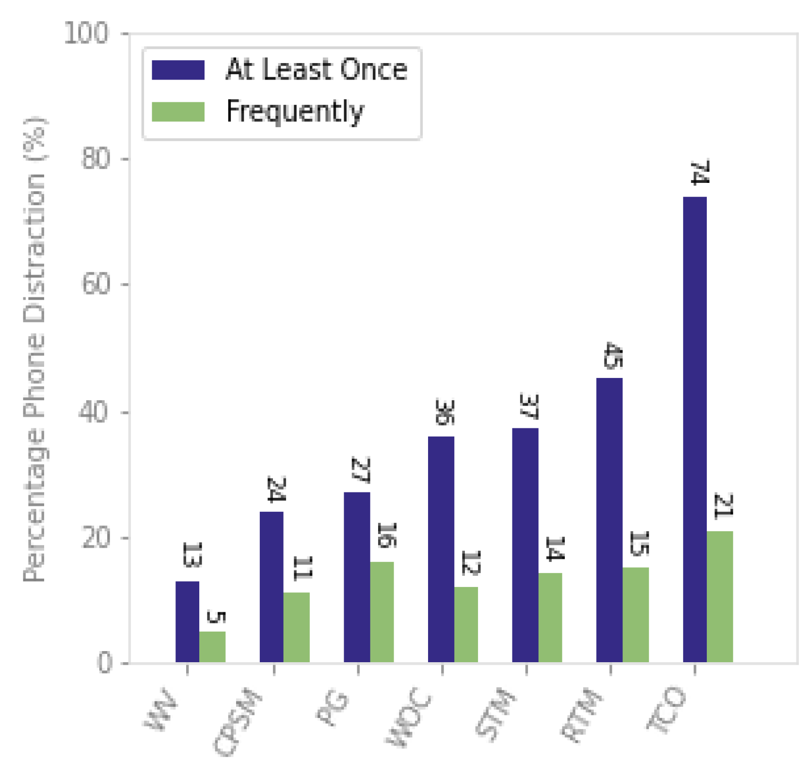
Distracted driving, including daydreaming, eyes off the road, and cell phone usage, accounts for a large proportion of road traffic fatalities worldwide. Out of these distractions, cell phone usage is at the top of the list as shown in Figure 1. Road traffic fatalities have been on the rise for the last few years [4]. In this regard, researchers have begun to explore the benefits of artificial intelligence when applied to a diverse range of problems, including, but not limited to, understanding driving behaviors, mitigating road incidents, and developing driver’s assistance systems [5,6].

The report also shows that the total number of deaths has been increasing each year and driver’s distraction is considered to be the leading cause of these accidents. Mobile phone usage during driving is widespread among novice and young drivers, which further adds more risk as shown in Figure 1.

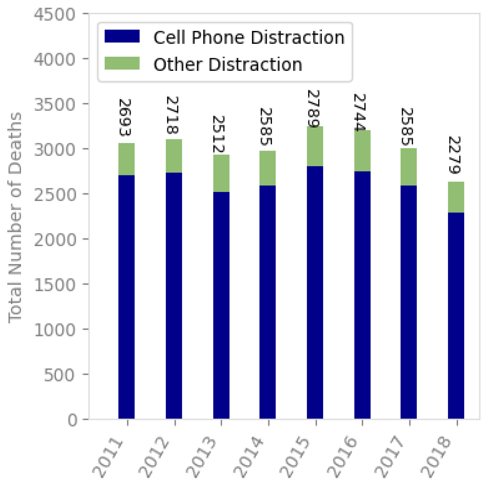
Around 200 applications for highway safety were developed by the American Automobile Association (AAA), that were used for head pose estimation, drowsiness and sleep detection, driver’s facial movement detection, and driver’s training [2]. Figure 2 shows the statistics based on the National Safety Council analysis of NHTSA data. It shows that, on average, 3022 deaths were caused by distracted drivers.

With the recent increase in computational resources, and a greater availability of parallel computing architectures, deep learning—that was previously considered infeasible—has now become possible and has demonstrated promising results for object detection [7,8], image classification [9,10], and other image analysis tasks [11,12].

As opposed to using handcrafted features, the automatic extraction of deep features has cause a paradigm shift towards the usage of convolutional neural networks. Various studies have used recurrent neural networks (RNNs) for extraction of spectral information [6] and convolutional neural networks (CNNs) for spatial information extraction [13,14] to classify various driving postures, and they yielded better results.

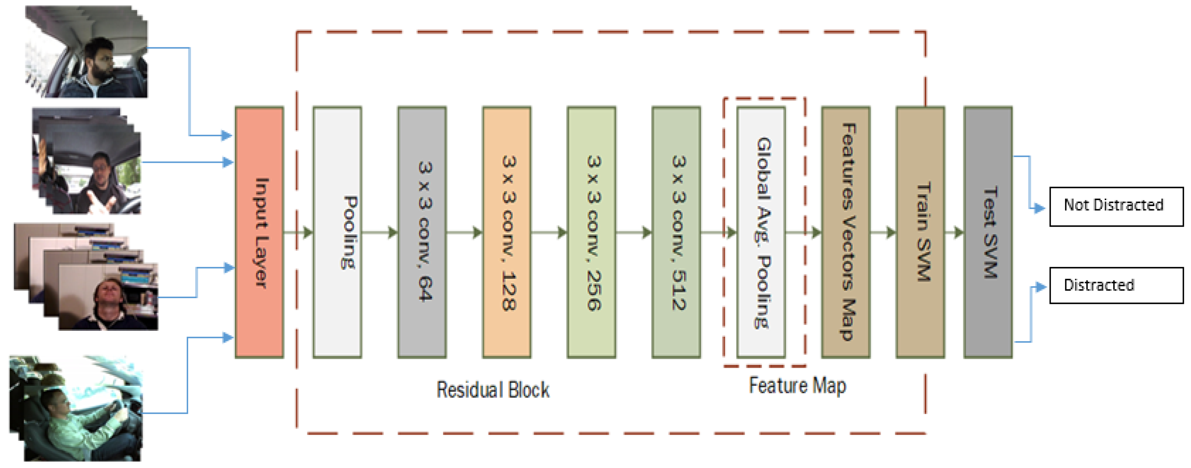
The study proposes ReSVM, an extension of our previous work [15], that uses deep features of ResNet-50 along with support vector machine (SVM) for identifying distracted drivers. The features from RGB frames are extracted from the average max-pooling layer after a series of convolutional and pooling batch normalization operations. A feature vector map is used for training and testing using SVM.

In this study, we have classified distracted drivers based on a single image. We take into account various types of distraction. A driver is distracted if he/she is texting, calling, turning on the radio, drowsy, sleepy, drinking, looking right, talking and laughing, waving a hand, looking down while driving, signaling, head nodding under varying lighting conditions, closing eyes, head panning under varying lighting conditions, has a sad and tensed face, watching the right direction, watching the back side, watching something low down while driving, and watching a distraction to the left. It should be noted that image classification takes into consideration only the spatial features. The temporal aspect is, however, ignored which reduces the complexity of the problem.

The datasets used in our experiments are State Farm Distracted Driver Detection (SFDDD), Boston University (BU), DrivFace, and FT-UMT datasets.

• An approach to detect driver distraction is proposed which uses the deep features of ResNet-50 that are then used by the SVM for the classification. To the best of our knowledge, we are the first to propose feeding deep features of ResNet to an SVM classifier.
• We evaluated our approach using four datasets, namely; State Farm Distracted Driver Detection, Boston University, DrivFace, FT-UMT.

  -

  We compared our proposed architecture with 12 existing approaches. Results showed that our proposed approach outperforms these approaches on these datasets in terms of accuracy.

  -

  Our proposed approach, based on deep features of ResNet-50, outperforms existing deep architectures.

The work is important since it has diverse applications impacting driver safety. It can be used by car manufacturers to implement safety features that will prevent accidents due to distraction. Businesses that manage large fleets of vehicles, such as those in the mobility, ride-sharing, and trucking industries, can use this to monitor their drivers for tiredness and distraction, and hence improve the work conditions, and ensure the safety of their workers. Law enforcement and highway safety agencies can use it to detect drivers that may pose a threat to the others on the road, and take actions to preempt any accidents.

The rest of this paper is organized as follows. Related work is discussed in Section 2 while proposed methodology and datasets are presented in Section 3 and Section 4.4, respectively. We share our evaluation results in Section 5.6 while variants of the proposed approach are illustrated in Section 6. Conclusions and future work are given in Section 9.

2. Related Work

The related work has been divided broadly into two main categories, machine learning and deep learning.

2.1. Approaches Based on Machine Learning

Zhang et al., in 2011, identified mobile usage as one of the major causes of driving accidents [16]. They implemented a hidden conditional random fields model based on mouth, facial, and hand features for profiling of cell phone usage by the drivers. They were able to achieve 91.2% accuracy. Zhao et al. proposed a feature-based approach using contourlet transform (CT), skin-like region segmentation, and homomorphic filtering using a random forest classifier for detecting distraction [17]. Their approach was developed for classifying four activities, namely: operating the shift gear, grasping the steering wheel, eating, and talking on a mobile phone. It was empirically observed that eating was the most difficult category to classify. Their approach yielded 88% accuracy on their self-generated dataset at Southeast University (SEU). Zeng et al. proposed an approach based on Haar-like features to detect the driver’s eye state and head movement, exhibiting 80% accuracy [18].

Image classification approaches are usually computationally intensive. To address this issue, Wang and Qin presented an architecture which used FPGA for faster image processing [19]. Their objective was to determine if the drivers’ eyes were closed in the image. They combined grayscale projection with Prewitt operator-based edge detection for the classification. Sigari et al. implemented various features including facial features, eye gaze direction, and head pose estimation on a Raspberry Pi [20]. They used these features along with a support vector machine for distraction detection. Liu et al. proposed a real-time system using the driver’s head and eye movement for detecting cognitive distraction [21]. They proposed a semi-supervised method to increase the time efficiency of labeling the training data. Seshadri et al. proposed a framework using histogram of gradients along with adaptive boosting, and yielded 93.9% accuracy on their self-generated dataset [22].

Ragab et al. proposed a distraction detection system based on five visual cues using a random forest classifier and achieved an accuracy of 82.78% [23]. These cues included eye closure, arm position, eye gaze, orientation, and facial expression. Liao et al. proposed a real-time algorithm for detection of cognitive distraction using a support vector machine (SVM) [24]. They evaluated their approach on self-generated datasets, achieving an accuracy of 98.5% and 93.0% for urban and highway simulated scenarios, respectively. Streiffer et al. proposed an approach based on random forest and contourlet transform for distraction detection [25]. They tested their approach on a dataset that was generated using the driver’s side pose and achieved an accuracy of 90.5%.

Wathiq et al. [26] presented a two-pronged approach in which the system first determines if a driver was distracted, based on yawing, head position, eye position, mouth position, etc. In the case of distraction, an alarm was generated and nearby hospital services were informed so that they could remain ready for any mishaps. They developed various features for face orientation, arm position, facial expression, and eye behavior. These features were combined and fed to the feed-forward neural network (FFNN). Their approach achieved a classification accuracy of 95.62.

Along similar lines, in 2019, Ou et al. proposed a deep neural network for the detection of distracted driving [27]. The system also worked in night mode using a near-infrared camera and achieved 92.24% accuracy. In daylight, the accuracy improved to 95.98%.

In 2017, Li et al. presented an architecture to investigate the solutions for distracted driving using performance indicators from on-board kinematic readings [28]. They developed a non-linear autoregressive exogenous (NARX) driving model to predict vehicle speed using distance headway and speed history. In the end, two features, mean absolute speed prediction error and steering entropy from the NARX model, were used with the SVM, yielding an accuracy of 95%.

2.2. Approaches Based on Deep Learning

Deep learning networks have shown promising results towards solving computer vision problems in the last decade [29,30]. Wollmer et al. implemented an LSTM recurrent neural network for real-time detection of driver’s distraction, head tracking, and modeling the temporal context of long-range driving [31]. They were able to implement subject-independent detection of inattention. Ren et al. used the Faster-RCNN deep learning model [32] and obtained an accuracy of 94.2% on the dataset developed by Seshadri et al. [22]. Streiffer et al. proposed a deep learning architecture, DarNet, that used the sensor data as an input for the classification of driving behavior [25], yielding better results than the baseline model.

In 2016, Le et al. proposed an R-CNN model to detect the hand position on the steering wheel [33]. In the same year, Yuen et al. implemented AlexNet for head pose estimation and used the stacked hourglass network in the refinement stage to predict facial landmarks and reduce the face localization [34]. They classified distraction based on the yaw angle of the driver’s head [35].

In 2017, Kim et al. proposed an architecture to classify open and closed eye images with different conditions, acquired by a visible light camera, using a deep residual convolutional neural network [36]. In the same year, Whui Kim et al. made a comparison of various deep learning networks including Inception, ResNet-50, and MobileNet using the ImageNet Large Scale Visual Recognition Challenge (ILSVRC) 2012 dataset [13]. Their key insight was that the MobileNet outperformed the other networks.

In 2018, Masood et al. implemented VGG-16 to identify the cause of distraction and achieved an accuracy of 99% on the State Farm Distracted Driver Detection (SFDDD) dataset [37]. In the same year, Tran et al. [38] developed an assisted driving testbed to create realistic driving experiences and validate the distraction detection algorithms. They used four CNNs, AlexNet, VGG-16, ResNet, and GoogLeNet, that were implemented and evaluated on an embedded GPU platform. They also developed a warning system for alerting the distracted driver in real time. Another distraction detection system based on convolutional neural network and data augmentation techniques was proposed by Sathe et al. whose main purpose was to decrease overfitting and increase the variability of the dataset [39].

In 2019, Xing et al. proposed a CNN model based on a Gaussian mixture model (GMM) for recognition of driver’s behavior [40]. To minimize the training cost, transfer learning was applied before training the model. They used three CNN models, namely: GoogLeNet, AlexNet, and ResNet-50. The authors focused on classifying various activities including texting, rear and side mirror checking, answering a cellular phone, talking, and using an in-vehicle radio device. They were able to achieve an 81.6% accuracy using AlexNet, and a lower accuracy of 78.6% and 74.9% using GoogLeNet and ResNet50, respectively. They were able to achieve 78.6%, 81.6%, and 74.9% using AlexNet, GoogLeNet, and ResNet-50, respectively.

More recently, Mase et al. empirically observed that Inception-V3 coupled with bidirectional LSTMs outperformed other CNN and recurrent neural network (RNN) architectures with an average F1-score of 93.1%. Their approach focused on identifying postures which were indicative of distraction. In 2020, Li et al. proposed a bimodular approach for distraction detection consisting of two modules on a self-generated dataset [41]. The first module computes the bounding box of the driver’s right ear and hand, and provides this as input to the second module. The second module of the proposed approach used the input information to predict the distraction type. Dhakate et al. proposed an ensemble method to detect distracted drivers by stacking the feature vectors of various convolutional networks [42].

The Boston University (BU) dataset consists of images that cover four types of distractions, namely: looking down, head nodding, eye closure, and head panning. These images have been generated in controlled lab settings where the light source was moved in different directions while capturing the images. Dahmane et al. proposed a distraction detection system based on yaw head pose estimation using the BU dataset [43]. Later, in 2017, they proposed a system to estimate both roll and yaw angle using a decision tree model [44]. They used non-intrusive feedback regarding the user’s head pose in order to determine the direction of their gaze and subsequently infer their attention level. Eraqi et al. proposed an approach which relied on a weighted and ensembled convolutional network [45]. They tested their approach on the BU dataset and obtained 84.64% accuracy. In 2018, Ali and Tahir proposed a feature-based system using a neural network to detect distraction due to driver’s head panning, achieving an accuracy of 89.20% on the same dataset [46]. In the BU dataset, our proposed approach ReSVM, combining deep features of ResNet-50 with an SVM classifier, outperforms the state-of-the-art approach (89.20%) by achieving an accuracy of 90.46%. However, this dataset lacks more realistic scenarios. Compared to the BU dataset, SFDD and DrivFace datasets contain more realistic images as well as more categories of distraction.

Hssayeni et al. relied on deep convolutional methods on dashboard camera images to detect distracted drivers [47]. They used transfer learning on AlexNet, VGG-16, and ResNet-152 and were able to achieve an accuracy of 82.5% on the SFDD dataset. In 2018, Chawan et al. proposed a system based on averaging the various existing convolutional neural network (CNN) models, namely: VGG16, VGG19, and Inception, for classification of distracted drivers [48]. They achieved an accuracy of 89.9% on the same dataset. In 2020, Mse et al. proposed a novel approach to identify distracted drivers from their postures using CNNs and stacked bidirectional long short-term memory (BiLSTM) networks which captured the spectral–spatial features of the images [49]. Results showed that they achieved a classification accuracy of 92.7% on the same dataset. In 2019, Tamas et al. proposed that the dropout layer from VGG-16 could be used to prevent overfitting while detecting driver’s distraction [50]. In addition to that, an attention mechanism was implemented to optimize the resource allocation. The authors tested various activation functions, including DReLU, SELU, and Leaky ReLU, and achieved 95.82%. accuracy on the SFDD dataset. In 2020, Vijayan et al. gave a comparative analysis of the approaches called scale invariant feature transform (SIFT) and RootSIFT for drowsy feature extraction [51]. The enhanced SIFT, called RootSIFT, achieves 93% accuracy on the BU dataset, which is better than normal SIFT in extracting the drowsy features. In 2020, Ortega et al. introduced the Driver Monitoring Dataset (DMD), an extensive dataset which includes real and simulated driving scenarios: distraction, gaze allocation, drowsiness, and hand–wheel interaction [52]. They achieved an accuracy of 93.2% on the same dataset. Previously, in 2016, Diaz et al. proposed a new automatic method for coarse and fine head yaw angle estimation of the driver [53]. They relied on a set of geometric features computed from just three representative facial keypoints, namely the center of the eyes and the nose tip. They were able to achieve an accuracy of 81% on the BU dataset. Although these aforementioned approaches exhibited good accuracy, there is still room for improvement. Our proposed approach, ReSVM, outperforms the state-of-the-art approaches and achieves an accuracy of 95.5% and 93.44% on SFDD and DrivFace datasets, respectively. One of the reasons why our approach outperforms the state-of-the-art techniques is because ResNet performs well with noisy data as compared to the other CNNs.

3. Methodology

This study proposes a deep learning architecture, ReSVM, for driver’s distraction detection. ReSVM is an optimized version of ResNet-50 that uses deep features obtained by the latter’s pooling layer and feeds these features to a support vector machine (SVM) as can be seen in Figure 3.

Previously, deep learning architectures, such as CNNs, could only use sigmoid functions for various computer vision tasks. Therefore, there was a limit on the number of layers of these networks. More recently, with the introduction of rectified linear unit, AlexNet and VGGNet have been able to use an increased number of layers i.e., 5 and 19, respectively. The increase in the number of layers resulted in an increase in training error. Later on, this degradation problem was addressed with the development of residual networks (ResNets) [30].

A large number of training samples from the ImageNet dataset were used for training a residual neural network (ResNet-50) to classify a diverse range of images including living things such as animals, birds, rodents, etc., and also various inanimate objects. The residual networks, with 50 or 101 layers, use residual blocks in their network architecture [30] and have consecutive 1 × 1, 3 × 3, and 1 × 1 convolution layers. Normally, deep ResNet layers contain 3 × 3 filters. Feature size is inversely proportional to the number of filters, i.e., if the feature map size is doubled, then the number of filters is reduced to half and vice versa. Due to this relationship, the time complexity is conserved.

The ReSVM takes an input of images with different sizes and variable lighting conditions as shown in Figure 3. The basic idea is to stack all the features as a feature map that is obtained from the last multilayer perceptron convolution layer (mlpconv) of the trained ResNet-50. Then, mean of the feature map is computed and fed to the SVM layer for classification [54].

Global average pooling carries several advantages over fully connected layers. For one, it is more native to the convolution structure because it enforces correspondence between feature maps and different categories [55]. An overfitting at this layer is avoided as there exists no parameter that needs optimization in case of global average pooling. The spatial information is summed up in case of global average pooling, which makes it more robust to spatial translations of the input.

SVM has been in use for the last couple of decades owing to its accurate classification with lower computational costs and excellent generalization ability [56,57]. A non-linear approximation and adaptive learning capability of SVM brings various benefits in handling non-linear data and small samples [58]. SVM is suitable for both regression as well as classification tasks. The SVM algorithm finds a hyperplane by classifying the data points in an N-dimensional space. The objective of the SVM algorithm is to find a maximum separating margin between the hyperplane and the data points. For maximizing the margins, hinge loss is used as a loss function. Our experimental results clearly show that SVM (with non-linear RBF kernel [59]) used with our architecture outperforms a neural network (MLP) on all four datasets. This improvement can be attributed to some inherent strengths of SVMs. Namely, they have good generalization capabilities which prevent overfitting, and they can also handle non-linear data efficiently. In the case of artificial neural networks, there is no specific rule for determining their structure. The appropriate network structure is achieved through experience and trial and error. It can further be observed that SVM also exhibits better results as compared to ID3, AdaBoost, naive Bayes, random forest, and k-NN.

• Training data $\{{\mathbf{x}}_i,y_i\}i=1,\dots ,l$, ${\mathbf{x}}_i\in {\mathbb{R}}^n$, and $y_i\in \{-1,1\}$.
• On a separating hyperplane: $\mathbf{x}\mathbf{w}+b=0$, where

  -

  w normal to the hyperplane;

  -

  ${\displaystyle \frac{\left|b\right|}{\parallel \mathbf{w}\parallel }}$ is the distance to origin;

  -

  $\parallel \mathbf{w}\parallel$ Euclidean norm of $\mathbf{w}$.

• $d_{+}$, $d_{-}$ shortest distances from labeled points to hyperplane.
• Define margin $m=d_{+}+d_{-}$.
• Task: find the separating hyperplane that maximizes m.

Key point: Maximizing the margin minimizes the VC dimension.

• For the separating plane:

  $$\begin{array}{cc}\hfill {\mathbf{x}}_i\mathbf{w}+b\ge +1,& y_i=+1\end{array}$$

  (1)

  $$\begin{array}{cc}\hfill {\mathbf{x}}_i\mathbf{w}+b\le -1,& y_i=-1\end{array}$$

  (2)

  $$\begin{array}{c}\hfill \equiv \end{array}$$

  (3)

  $$\begin{array}{cc}\hfill y_i({\mathbf{x}}_i\mathbf{w}+b)-1\ge 0,& \forall i.\end{array}$$

  (4)
• For the closest points the equalities are satisfied, so:

  $$d_{+}+d_{-}=\frac{|1-b|}{\parallel w\parallel }+\frac{|-1-b|}{\parallel w\parallel }=\frac{2}{\parallel w\parallel }.$$

  (5)
• One coefficient per training sample.
• The constraints are easier to handle.
• Training data appear only in dot products.
• Great for applying the kernel trick later on.
• Minimize

  $${\displaystyle L_P=\frac{{\parallel w\parallel }^2}{2}-\sum _{i=1}^l{\alpha }_i{y}_i({\mathbf{x}}_i\mathbf{w}+b)+\sum _{i=1}^l{\alpha }_i.}$$

  (6)
• Convex quadratic programming problem with the dual: maximize

  $${\displaystyle L_D=\sum _{i=1}^l{\alpha }_i-\frac{1}{2}\sum _{i,j=1}^l{\alpha }_i{\alpha }_j{y}_i{y}_j\left({\mathbf{x}}_i{\mathbf{x}}_j\right).}$$

  (7)
• Those points having ${\alpha }_i>0$ represent the support vectors.
• Solution is mainly dependent on them.
• The points with ${\alpha }_i=0$ can be removed, or moved away arbitrarily from the hyperplane.
• Once the hyperplane is found:

  $$\widehat{y}=(\mathbf{w}\mathbf{x}+b).$$

  (8)

The optimal hyperplane is determined by solving the constrained optimization problem $min\left(\frac{1}{2}{w}^{T}w\right)$, subject to $y_n(w^T{x}_n+b)\ge 1$ for $n=1,2,3,\dots ,N,w\in {\mathbb{R}}^d,b\in \mathbb{R}$.

A way to find the non-linear classifiers’ kernel trick is applied to maximum-margin hyperplanes. In the resulting algorithm, a non-linear kernel function replaces every dot product, which enables it to locate the max-margin hyperplane in a new (mostly higher dimensional) feature space, essentially the transformed feature space. It can be a non-linear transformation and the new dimension can be of a higher dimension. The classifier in this space is linear, however, in the original input space, it can be non-linear. Although the generalization error increases in high-dimensional feature space, the algorithm still yields better results.

4. Datasets

We generated results on the four publicly available standard datasets given below to establish reliability of our approach and provide a comparison with state-of-the-art techniques. Since these datasets provide a broad coverage of the various types of distraction, by performing well on all of these, we establish that our approach can cater to a wide variety of scenarios.

Various state-of-the-art approaches have generated results on specific datasets. In order to provide fair comparison with those aforementioned approaches, we had to generate results on those datasets as well. Moreover, these datasets provided sufficient coverage of different activities that can be used to classify distraction detection.

4.1. State Farm Distracted Driver Detection

The study used the State Farm Distracted Driver Detection dataset (SFDDD) (https://www.kaggle.com/c/state-farm-distracted-driver-detection, accessed on 19 June 2022). It consisted of 2D images from dashboard cameras. A total of 22,400 images, having a resolution of 640 × 840 pixels, were used in the experimentation. Out of these, 21,000 images contained a distracted driver. A detailed breakdown is given in

Table 1. Distracted and not distracted frames in four datasets, namely: (i) SFDDD, (ii) BU, (iii) DrivFace, and (iv) FT-UMT. DF = Distracted Frames, NDF = Not Distracted Frames, TF = Total Frames.

Datasets	DF	NDF	TF
SFDDD	21,000	3000	22,400
BU	2178	1995	4173
DrivFace	391	216	607
FT-UMT	11,000	10,000	21,000

. The dataset was divided into 20,400 training images and 2000 testing images. As shown in Figure 4, the dataset contained various activities that were indicative of distraction, namely: (i) texting, (ii) operating the radio, (iii) making phone calls, (iv) drinking, (v) combing, (vi) applying makeup, and (vii) talking.

4.2. Boston University Dataset

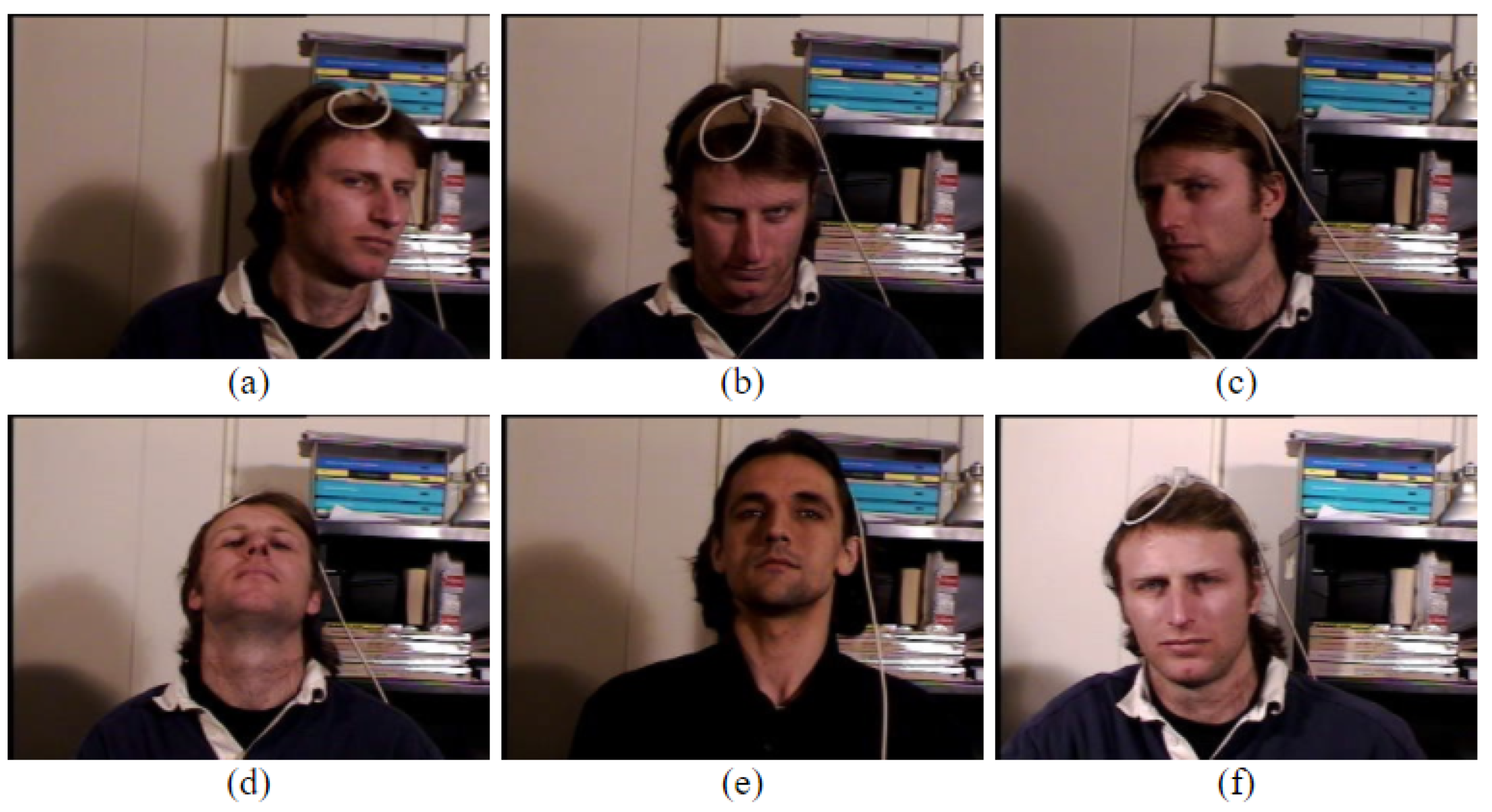
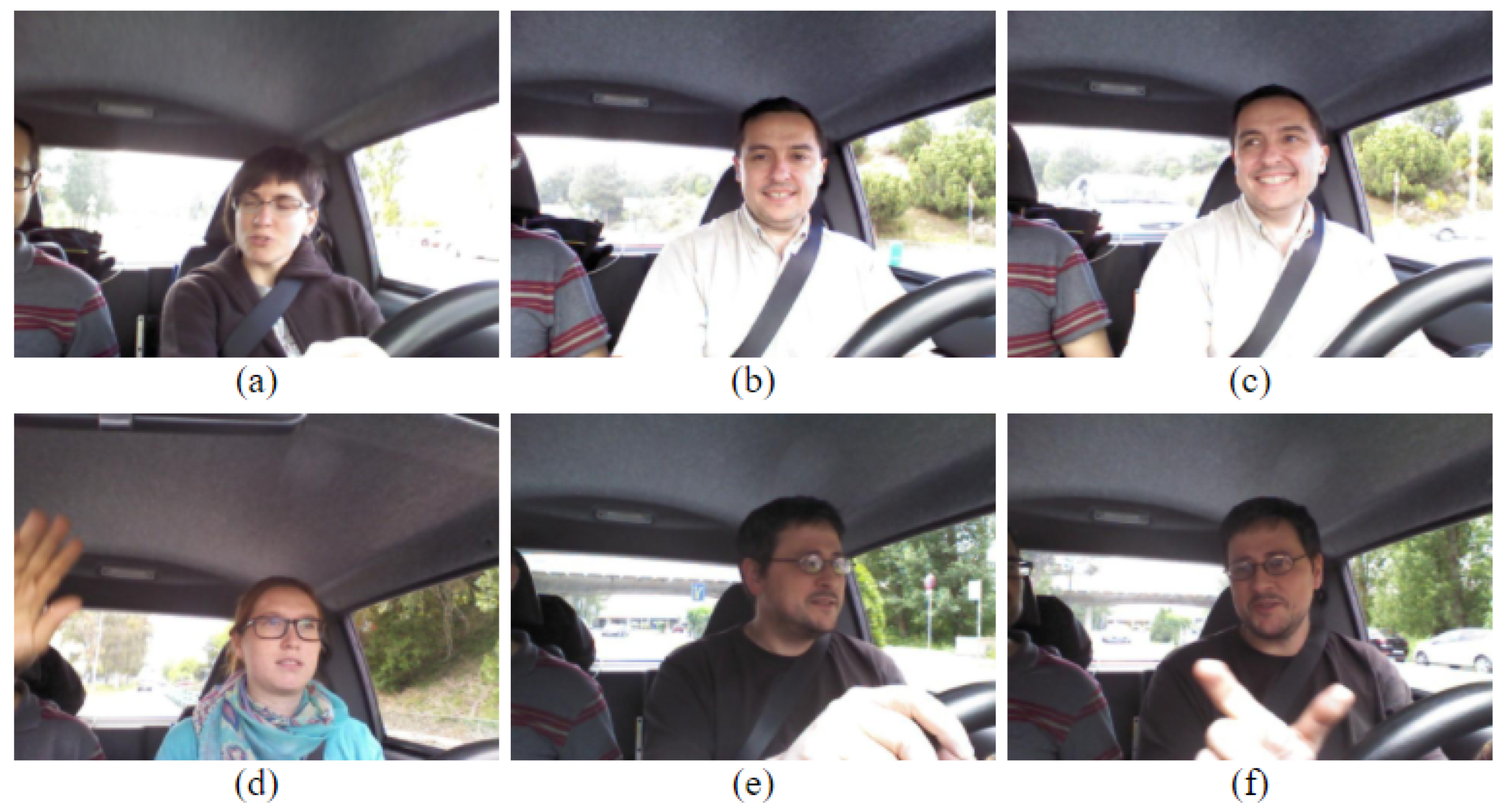
The study also used the Boston University dataset (BU) (http://csr.bu.edu/headtracking/, accessed on 19 June 2022) that, similar to SFDDD, consisted of 2D dashboard camera images. We used 4173 images, having a resolution of 320 × 240 pixels, for evaluation purposes. Out of these, 2178 images contained variation in the light conditions. This is shown in Table 1. The dataset was split into training and testing, consisting of 2000 images. The dataset contained various activities, namely: (i) varying light in left direction, (ii) varying light in right direction, (iii) varying light in up direction, (iv) nodding head with varying light, (v) watching up with varying light, as shown in Figure 5.

4.3. DrivFace Dataset

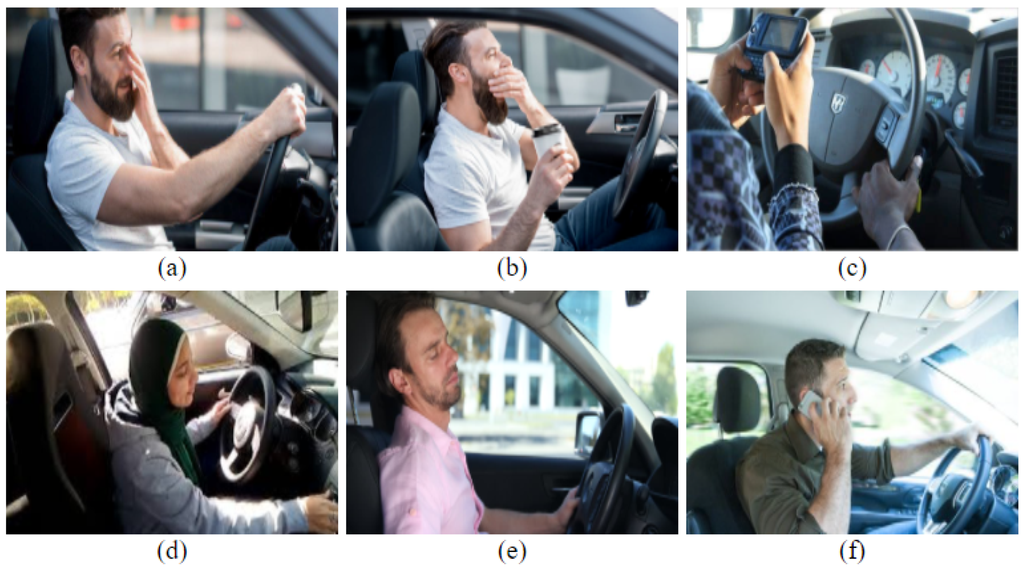
We used the DrivFace dataset (http://adas.cvc.uab.es/elektra/enigma-portfolio/cvc11-drivface-dataset/, accessed on 19 June 2022) that consisted of dashboard camera images. From it, 607 images with a resolution of 640 × 480 pixels were used in the experimentation. Out of these, 391 images depicted distraction as shown in Table 1. The dataset was divided into two parts: training and testing. Eighty percent of images were used for training and 20% for testing. The dataset contained various activities, namely: (i) talking, (ii) waving a hand, (iii) watching left direction, (iv) watching right direction, (v) nodding head, (vi) setting on the dashboard, and (vii) sleeping, as shown in Figure 6.

4.4. FT-UMT Dataset

Lastly, the study used the FT-UMT dataset (https://sites.google.com/site/farooq1us/dataset, accessed on 19 June 2022) consisting of 2D dashboard camera images. A total of 21,000 images were used. These had a resolution of 640 × 480 pixels. Out of these total frames, 11,000 contained a distracted driver, as is shown in Table 1. The dataset depicted various activities, including: (i) looking left, (ii) sad and tensed face, (iii) drowsiness, (iv) watching back direction, (v) nodding the head, (vi) looking right, and (vii) sleeping.

5. Experiments and Results

The proposed architecture, ReSVM, was compared with ResNet-50, ResNet-101, VGG-19, MobileNet, InceptionV3, and Xception for a two-category problem of driver’s distraction detection. The first category corresponds to normal driving without distraction, while the second corresponds to distracted driving that may include talking on a phone, texting, drinking, operating the radio, talking, combing, and applying makeup. We evaluated the classification accuracy and the execution time of our approach on four publicly available datasets, namely: State Farm Distracted Driving (SFDDD), Boston University (BU), DrivFace, and FT-UMT datasets using 10-fold cross validation.

The parameter ranges used for ResNet-50, ResNet-50, ResNet-101, VGG-19, MobileNet, InceptionV3, and Xception classifier are dropout = ‘0.1’, activation function = ‘softmax’, and optimizer = ‘rmsprop’.

5.1. Experimental Setup

Experiments were performed using Google Colab. The hardware consisted of an NVIDIA Tesla K80 GPU with 16 GB of graphics memory. The code was written in Python.

5.2. Experiment 1: State Farm Distracted Driver Detection Dataset

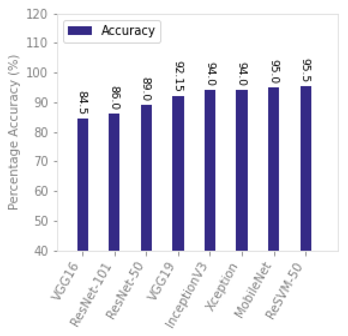
ReSVM outperformed the existing state-of-the-art approaches on SFDDD as can be seen from

Table 2. Comparison of ReSVM in terms of accuracy with existing architectures on four datasets, namely: (i) State Farm Distracted Driver Detection, (ii) Boston University, (iii) DrivFace, and (iv) FT-UMT datasets. DS = Dataset, D1 = SFDDD, D2 = BU, D3 = DrivFace, D4 = FT-UMT, R-50 = ResNet-50, R-101 = ResNet-101, V-19 = VGG-19, I-V3 = InceptionV3, M = MobileNet, Xp = Xception.

Ds	R-50	R-101	V-19	M	I-V3	Xp	ReSVM
D1	89.00	86.00	92.15	95.00	94.00	94.00	95.50
D2	87.30	44.44	47.09	60.32	86.24	85.71	90.46
D3	87.61	45.90	39.34	80.33	85.25	85.25	93.44
D4	82.50	54.50	48.50	94.00	92.00	91.50	94.50

and Figure 7. The reasons include the combination of deep features of ResNet-50 along with the SVM classifier in the ReSVM. SVM scales relatively well to high-dimensional data and also reduces the risk of overfitting [60]. This modification increased the percentage accuracy of the proposed approach from 89%, using simple ResNet-50, to 95.5%. It can be empirically observed that this combination was helpful for datasets containing high intraclass variations such as SFDDD. This dataset has a variety of distractions including texting, talking, operating the radio, nodding, panning, drinking, combing, applying makeup, and cognitive distractions.

Table 3. Optimal parameters (number of epochs and learning rate) of ReSVM and state-of-the-art deep networks. R-50 = ResNet-50, R-101 = ResNet-101, V-19 = VGG-19, I-V3 = InceptionV3, M = MobileNet, Xp = Xception.

Epochs/LR	R-50	R-101	V-19	M	I-V3	Xp	ReSVM
Epochs	20	60	70	20	20	20	20
LR	0.10	0.10	0.10	0.10	0.10	0.10	0.10

shows the optimal parameters (number of epochs and learning rate) of the proposed approach (ReSVM) and existing deep networks.

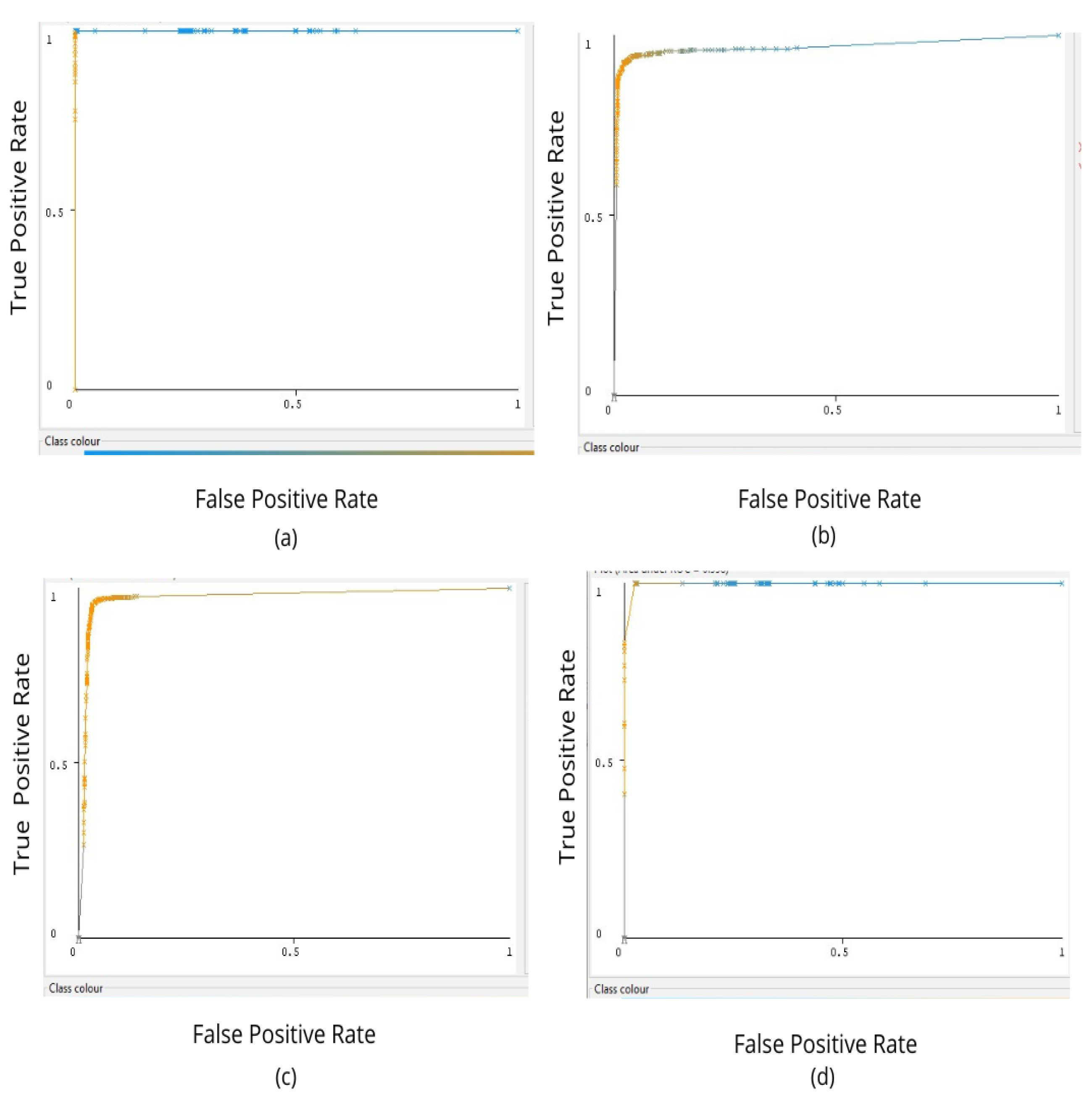
Figure 8 shows the ROC-AUC plot obtained by applying ReSVM on SFDDD, BU, DrivFace, and FT-UMT datasets. The value of AUC-ROC for the SFDDD dataset is highest, showing that ReSVM has the highest measure of separability. It shows that the proposed model is better in distinguishing between a distracted driver and one who is not distracted. The value ROC-AUC for BU and DrivFace datasets is relatively lower than that of SFDDD. The reasons include the dim light conditions, lack of clarity, and high intraclass variations of these datasets.

5.3. Experiment 2: Boston University Dataset

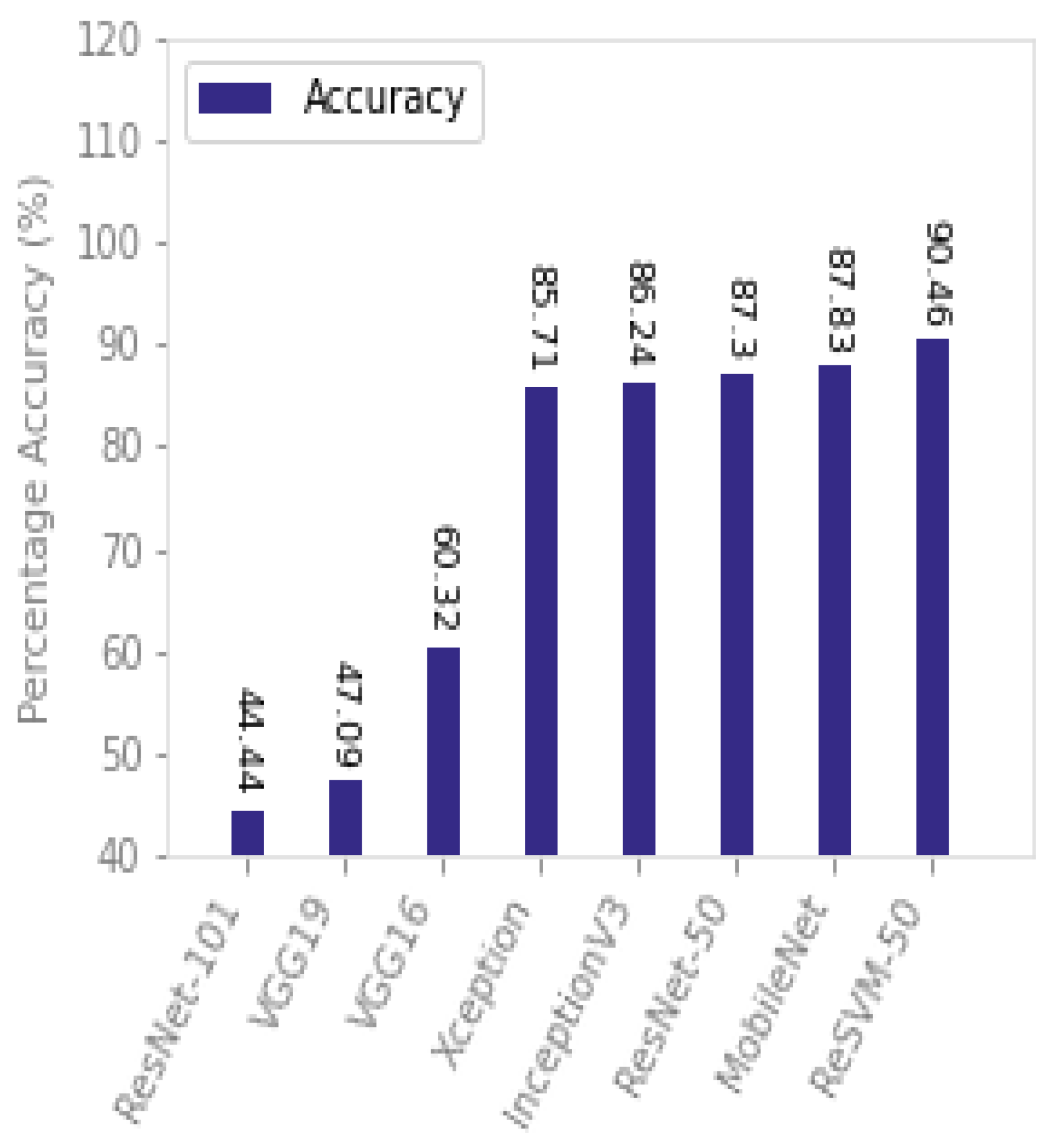
ReSVM outperformed the state-of-the-art approaches on the Boston University dataset as can be seen from Table 2 and Figure 9. As can be observed, the accuracy of ResNet-50, ResNet-101, VGG-19, MobileNet, InceptionV3, and Xception are reduced drastically in this dataset as compared to SFDDD. For instance, the percentage decrease in accuracy of VGG-19, ResNet-101, and ResNet-50 is {47.09%, 44.44%, and 87.15%}, respectively. This is due to dim light conditions and lack of clarity in the frames of this dataset. However, ReSVM-50 remained comparatively stable with a percentage decrease of 3.31%. Both ReSVM-50 and ResNet-50 use the same deep features, however, they differ in classifier. The combination of deep features of ResNet-50 along with the SVM classifier is responsible for this stable performance of ReSVM. One reason includes the ability of the SVM classifier to show good performance on small samples and large features [61]. The accuracy of VGG-19 drastically decreases in this dataset as compared to SFDDD. One reason for this degradation in performance is the lack of a large amount of training data [62].

5.4. Experiment 3: DrivFace Dataset

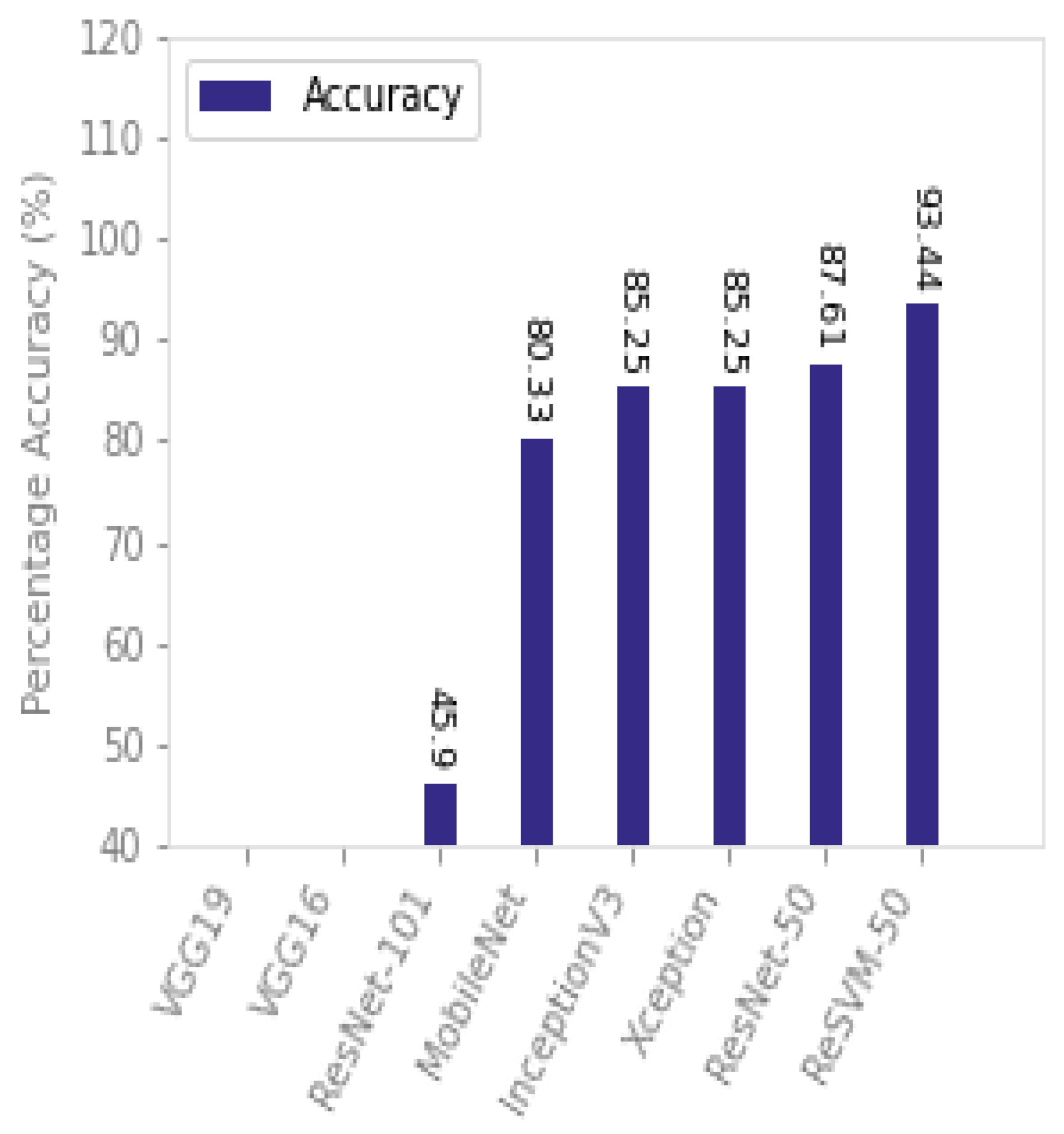
Once again, ReSVM outperformed the state-of-the-art approaches when tested on the DrivFace dataset as can be seen from Table 2 and Figure 10. All the approaches, including proposed and existing, underwent the same percentage degradation as can be seen in the case of the BU dataset. For instance, the percentage decrease in accuracy of VGG-19 and ResNet-101 was 57.30% and 46.63%, respectively. The dataset is smaller in size and has high intraclass variations due to the illumination factor of frames, glasses, eye gaze movements, talking to a passenger, picking up something on the dashboard, sleeping, etc. It can further be observed that ReSVM replaces the SVM classifier in ResNet-50, which increases its accuracy from 87.61% to 93.44%. As mentioned in Section 5.3, the SVM classifier shows good performance on small samples and large features [61].

5.5. Experiment 4: FT-UMT Dataset

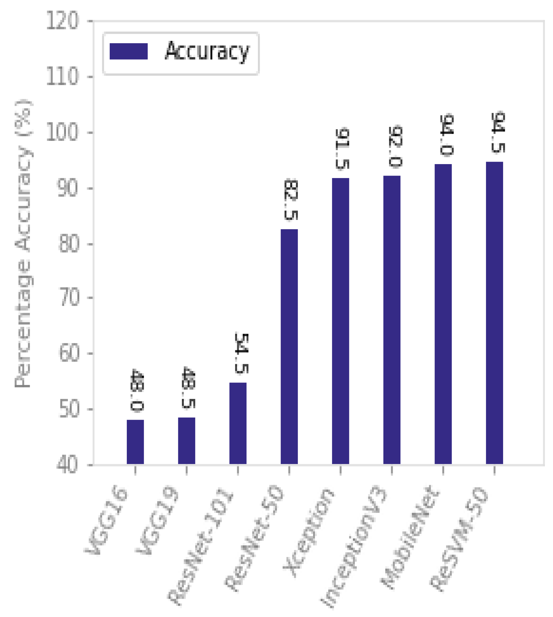
As opposed to the other datasets considered in this study, the FT-UMT dataset poses more challenges because it also takes into account the user expressions, such as sadness and anger, which increases the intraclass variations. As can be seen in Table 2 and Figure 11, ReSVM exhibits the best performance accuracy as compared to the other approaches on this dataset.

5.6. Experiment 5: Execution Time

We compared the running time of our approach with the state-of-the-art on four datasets, namely: (i) State Farm Distracted Driver Detection, (ii) Boston University, (iii) DrivFace, and (iv) FT-UMT. It can be observed from

Table 4. Comparison of proposed approach i.e., ReSVM, in terms of time with existing architectures on four datasets. T(s) = Time.

Ds	R-50	R-101	V-19	M	I-V3	Xp	ReSVM
D1	40	840	86,700	6840	18,540	35,100	720
D2	200	560	53,040	4920	12,600	22,920	613
D3	60	120	114,60	1050	2130	4380	951
D4	160	420	45,210	3810	9810	17,010	902

that ReSVM is 120, 10, 26, 49 times faster than VGG-19, Mobile-Net, InceptionV3, and Xception, respectively, on SFDDD while it is {141, 11, 30, 57} times faster in the case of the BU dataset. A similar trend is observed in DrivFace and FT-UMT datasets. The best execution time was achieved by ResNet-50 but at the cost of reduced accuracy. Our proposed approach, ReSVM, uses similar deep features as that of ResNet-50 but it differs in the use of the classifier. It can be observed from Table 2 that the usage of this SVM classifier increases its percentage accuracy from {89, 87.15, 87.61, 82.50} in the case of ResNet-50 to {95.5, 90.46, 93.44, 94.5} on SFDDD, BU, DrivFace, and FT-UMT, respectively, however, the execution time increases as well.

6. Variants of Proposed Approach

We also explored the impact of replacing the SVM with other classifiers in our proposed approach ReSVM. More specifically, we explored the effect of using ID3, multilayer perceptron (MLP), AdaBoost, naive Bayes (NB), random forest (RF), and k-nearest neighbor (k-NN) classifiers on SFDDD, BU, DrivFace, and FT-UMT. The parameters of these approaches are shown in

Table 5. Parameters used for comparison of decision tree, random forest, k-NN, AdaBoost, and MLP.

Classifier	Parameters
Decision Tree	criterion = ‘entropy’
	in_samples_split = 2
	random_state = 0
	splitter = ‘best’
Random Forest	parcriterion = ‘entropy’
	n_estimators = 10
	random_state = 0
k-NN	leaf_size = 30
	metric = ‘minkowski’
	n_neighbors = 5
	p = 2
	weights = ‘uniform’
AdaBoost	n_estimators = 50
	random_state = None
MLP	activation = ‘relu’
	alph = 0.0001
	max_fun = 15,000
	max_iter = 50
	random_state = 0
	solver = ‘adam’

. In all experiments, ReSVM was seen to outperform other classifiers as shown in

Table 6. Comparison of four datasets with state-of-the-art in terms of percentage accuracy in variants of proposed approach.

Ds	SVM	ID3	MLP	AB	NB	RF	k-NN
D1	95.50	77.50	84.00	33.00	73.00	91.50	91.00
D2	90.46	75.60	59.78	48.67	57.14	86.70	87.30
D3	93.44	73.77	72.13	62.29	75.40	88.50	86.88
D4	94.50	88.50	81.00	80.50	76.50	95.50	94.00

.

It can be observed that the SVM outperformed the other approaches in all four datasets. The ID3 algorithm exhibited lower accuracy compared to ReSVM as it suffered from overfitting. The degradation in MLP performance is due to the fact that it is hard to train and requires a large amount of training data. Naive Bayes implicitly assumes that all the attributes are mutually independent. This might not always hold true—thereby limiting its application in many scenarios. Random forest and k-NN are computationally very expensive in large datasets—the former due to the fact that it creates a lot of trees (unlike only one tree in the case of decision tree), while the latter suffers because it requires calculating distance for each data instance. They are also sensitive to noisy and missing data.

7. Comparison with Existing Approaches

We now present ReSVM’s improvement over the results presented in the existing literature.

Table 7. Comparison using SFDDD dataset.

Dataset	Chawan [48]	Mase [49]	Tamas [50]	Hssayeni [47]	ReSVM
SFDDD	89.90	92.70	95.00	85.00	95.50

shows that ReSVM outperforms Chwan, Mase, Tamas, and Hssayeni. It uses a combination of deep features of ResNet-50 and SVM that performs well on datasets containing high intraclass variations such as SFDDD.

ReSVM outperforms Eraqi, Ali, Dahmane2012, and Dahmane2015 in terms of percentage accuracy on the BU dataset as can be seen in

Table 8. Comparison using BU dataset.

Dataset	Eraqi [45]	Ali [46]	Dahmane [44]	Dahmane [43]	ReSVM
BU	85.00	89.20	79.63	81.40	90.46

. ReSVM uses an SVM that scales relatively well to high-dimensional data and also reduces the risk of overfitting [60]. It can be observed that all the approaches undergo a degradation in their percentage accuracy in this dataset as compared to SFDDD. One reason for this degradation in performance is the lack of a large amount of training data [62].

The dataset is smaller in size and has high intraclass variations due to the illumination factor of frames, glasses, eye gaze movements, talking to a passenger, picking up something on the dashboard, sleeping, etc.

Similarly, ReSVM outperforms Ali, Vijayan, Ortega, and Diaz as can be seen in

Table 9. Comparison using DrivFace dataset.

Dataset	Ali [46]	Vijayan [51]	Ortega [52]	Diaz [53]	ReSVM
DrivFace	92.35	93.00	93.20	81.00	93.44

.

8. Discussion

In this work, we compared our proposed approach with six networks (ResNet-50, ResNet-101, VGG-19, MobileNet, InceptionV3, and Xception) for a two-category classification problem of distraction detection (namely, texting—right, talking on the phone—right, texting—left, talking on the phone—left, operating the radio, drinking, reaching behind, hair and makeup, and talking to passenger distractions).

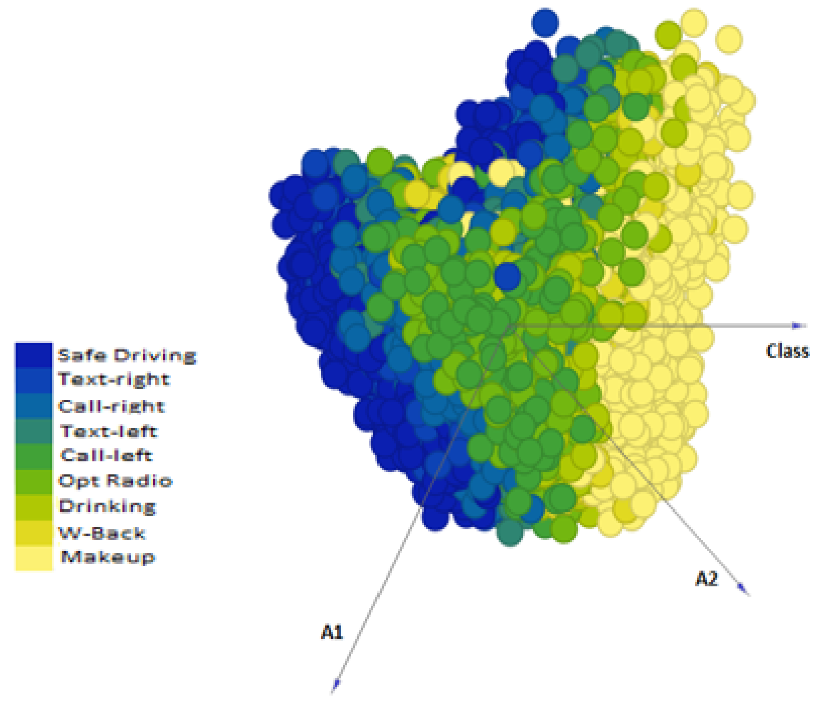
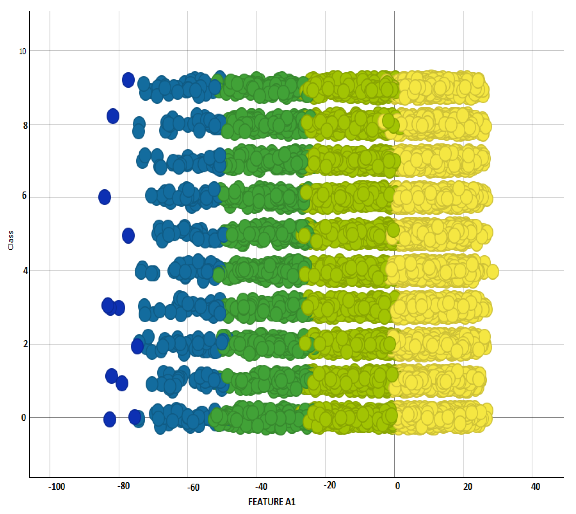
The proposed approach, based on the features obtained from the last pooling layer of ResNet-50 followed by the classification layer consisting of the SVM, outperformed the existing approaches and the state-of-the-art networks on SFDDD, DrivFace, BU, and FT-UMT detection datasets, as can be seen from the results presented in Section 6. Figure 7 shows that our proposed approach outperformed ResNet-50, ResNet-101, VGG-19, MobileNet, InceptionV3, and Xception, in terms of accuracy (with a maximum accuracy of 93.44%), whereas other methods exhibited lower accuracy with VGG-19 performing worst of all. The reason for the good performance of our proposed approach is the optimal classification capability of SVM on ResNet-50 features in Figure 12 and Figure 13 showing the scatter plot for the first two principal components of features extracted from ResNet-50. This figure gives the visualization of features of the SFDDD dataset that are obtained by applying principal component analysis. The low performance of VGG-19 is probably due to the vanishing gradient problem which is well addressed in the architecture of ResNet.

Table 10. Comparison of within-class (average distance) and between-class (average linkage) distances for SFDDD dataset.

Class	C0	C1	C2	C3	C4	C5	C6	C7	C8	C9
C0	0.00	0.50	1.50	2.50	3.50	3.50	3.50	3.50	3.50	3.50
C1	0.50	1.50	2.50	3.50	4.00	4.00	4.00	4.00	4.00	4.00
C2	1.50	2.50	0.50	2.75	3.60	3.90	3.80	3.80	2.50	2.90
C3	2.50	3.50	2.75	0.50	1.50	1.90	1.95	2.50	2.80	3.20
C4	3.50	4.00	3.60	1.50	0.50	0.50	1.90	2.10	2.30	3.10
C5	3.50	4.00	3.90	1.90	0.50	0.50	2.50	2.40	3.10	3.30
C6	3.50	4.00	3.80	1.95	1.90	2.50	0.50	0.50	0.50	0.50
C7	3.50	4.00	3.80	2.50	2.10	2.40	0.50	0.50	0.50	0.50
C8	3.50	4.00	2.50	2.80	2.30	3.10	0.50	0.50	0.50	0.50
C9	3.50	4.00	2.90	3.20	3.10	3.30	0.50	0.50	0.50	0.50

shows the interclass and intraclass distances for the features extracted from the last pooling layer of ResNet-50 for the SFDDD dataset. We can see that the interclass variation is higher than the intraclass variation, e.g., interclass distance of class 3 and class 4 is significantly higher than the intraclass distances shown in the diagonal. From the table, it can be seen that the interclass distance between classes 4 and 1 is maximum, i.e., 4. Equations (9) and (10) show the formulae for computing average distance and average linkage for intra- and interclass distances, respectively. In Table 10, the value 0.5 shows that the distance between those two classes is very small, i.e., high similarity exists. As there are many classes having high similarity, therefore, the value of 0.5 occurs frequently in the table.

$$S_a=\frac{{\sum }_{i,i^{{}^{\prime }}}\Vert x_i-x_{i^{\prime }}\Vert }{N_k(N_k-1)}$$

(9)

Here, $x_i$ is the number of intraclass feature attributes, $x_i-x_{i^{\prime }}$ is distance, and $N_k$ is total number of vectors.

$$d_a=\frac{{\sum }_{i,j}\Vert x_i-x_j\Vert }{N_k{N}_i}.$$

(10)

$x_i-x_j$ is distances of interclass vectors, $N_k{N}_i$ shows total number of vectors.

A question arises whether this approach would be feasible in a real scenario. If someone uses our pretrained network, then it can easily be deployed in a device with limited hardware. As is the case with all the machine learning and deep learning approaches, the training phase occupies a major chunk of computational resources and execution time. Once the model has been trained, the actual classification is not resource intensive and, hence, it can easily be deployed in hardware used in a car.

9. Conclusions and Future Work

In this paper, we proposed ReSVM, a residual neural network with an SVM classifier, for detecting various types of drivers’ distractions, including texting, operating the radio, drinking, talking on the phone, combing, and applying makeup.

We compared ReSVM with seven state-of-the-art approaches using four publicly available datasets. The results showed that ReSVM outperformed the other approaches and achieved a classification accuracy as high as 95.5%. ReSVM, obtained by replacing the ResNet-50 classifier with an SVM, showed a percentage improvement of {7.3, 3.31, 5.83, and 14.54} on SFDDD, DrivFace, BU, and FT-UMT, respectively, as compared to ResNet-50. This significant percentage increase in the BU dataset is due to that fact that SVM performs well on missing values and dim light datasets.

In future, we plan to explore additional features that can be useful for detecting distraction. Car motion can be an important indicator. For instance, a car swerving between lanes could imply distraction or driving under the influence of alcohol. Driver emotions, such as extreme anger, which have the potential to adversely affect the driver’s ability to drive safely, could be another strong indicator for distraction. Jittery limbs and other tics could also be useful for our purpose as they could imply tiredness or health issues.

In this paper, we performed the classification based only on the spatial features, i.e., on images. It is important to note that very short duration events, e.g., glancing down for a fraction of a second, might not be problematic, and hence should not be classified as distraction. These temporal aspects of distraction will be explored in our future work.

We also plan to develop approaches for monitoring unsafe driving behavior which may help prevent accidents, as well as assist law enforcement agencies. Among other things, this could include traffic signal and rule violations, speeding, tailgating, and sudden acceleration/deceleration for no apparent reason. Eventually, we also plan to go live and develop a distraction detection and alerting system in cars and evaluate its actual performance on roads. The addition of large data repositories for deep architectures will also be our future goal.