Abstract
This paper proposes an energy trading framework for a combined heat and power (CHP) microgrid (MG) integrated with a Photovoltaic (PV) generation system. The parties involved in the CHP-MG energy market are a single MG operator (MGO) and multiple users with electric and thermal demand response (DR). The energy trading process between the MGO and users is formulated as a Nash bargaining game, where the users can bargain with the MGO regarding trading volumes and the prices of electricity and heat. The relationship between the Nash bargaining solution (NBS) and social welfare maximum is studied. A distributed optimization algorithm based on the alternating direction method of multipliers (ADMM) is adopted to achieve NBS. Case studies demonstrate the effectiveness of the proposed trading framework, and show the promotion of economic benefits.
1. Introduction
With the increasing attention to energy consumption, environmental pollution, and climate change, how to improve energy efficiency is becoming one of the most urgent issues in the world []. In recent years, energy optimization management of microgrids (MGs) with thermal and electrical demand has become a subject worthy of further study []. In particular, the Micro turbine (MT)-based combined heat and power (CHP) system is popularly used as distributed energy resources (DERs) in MG because of its ability to provide both electric and thermal energy. Moreover, the CHP system integrated with renewable energy sources (RES), such as photovoltaic (PV) systems, can complement each other in energy supply and reduce emissions caused by energy consumption [].
Generally, the operation strategy of the CHP system is determined by the MG operator (MGO), according to the thermal and electric energy demand of end-users, the economic benefits of the MGO, and the supply reliability of MG. Reference [] introduces an economic model predictive control model for CHP-based MG, where the CHP system is responsible for following the heat demand of smart buildings. In [,], the CHP system is used to reduce the operation cost of the energy supply system, considering the stochastic characteristics of RESs and the uncertainties of energy consumption demands. Reference [] proposes a solution to both generation scheduling and economic dispatch of the CHP system and heat-only unit in the on-grid and off-grid mode of an MG. Reference [] proposes a CHP system model for meeting different operational needs of MG, which consists of the energy supply for the on-grid mode and the frequency regulation for the off-grid mode. Reference [] studied CHP-based MG to address two conflicting objectives, including minimizing operating costs and reducing pollutant emissions. A robust short-term scheduling integration of CHP-based MG protects the system from high operation costs while considering undesired deviation of dynamical market prices [].
Furthermore, demand response (DR) is regarded as another effective way to improve the efficiency of energy utilization in MG, where end users can participate in the energy management of MG by responding to the energy prices or incentive mechanism []. DR achieves the role transition of end-users from passive energy consumers to active participants, who can adjust the size and operation time of load demand. Reference [] proposes a multiparty energy management framework for the joint operation of CHP and PV consumers with price-based DR. Reference [] proposes a DR program implemented in the stochastic programming of MG. The amount of responsive load can vary at different time intervals. By using DR, the energy management of MG can be modeled as an inner energy market with multi parties, in which the MGO is designed as an energy retailer, and the end-users are energy buyers []. However, by applying smart equipment in utility infrastructure, energy consumers can adjust the thermal load demand according to the comfortable degree of the indoor environment []. Study [] indicates that the adaptive thermal loads can be modeled as a DR solution for a future power grid. For CHP-based MG, the thermal DR could be considered inside to further improve the response ability of the end user. Thus, the management of MG energy will become more complex, differing from solely electricity energy management. For simplification, the heat- and electricity-coupled DR is defined as hybrid DR, which is rarely studied. In [], a hybrid DR model based on shiftable electric and cuttable thermal loads is constructed in a CHP-based MG. The energy trading between MGO and hybrid DR users is modeled as a Stackelberg game, where the MGO determines the prices of electric and thermal energy, and users respond to the prices by shifting the electric demands and cutting off thermal demands. In [], the hybrid DR is applied to MGs, which participate in electric and thermal energy sharing in the distribution network. In this paper, a Nash bargaining cooperation game model was built to solve the multiparty energy management of CHP-based MG with hybrid DR. In [], a generalized Nash game model is built in this paper to simulate the multi-round auction in combined heat and power market (CHPM), where the consumer demand curves are deduced from the partial derivatives of their payoff functions, and the thermal comfort of the consumers is considered in their payoff functions. In [], an energy management framework is established for a multi-energy industrial park based on Stackelberg game theory, where the leaders and the followers are combined heat-and-power (CHP) unit owners and a group of industrial users. Compared with the non-cooperation strategy in [], the Nash bargaining cooperative game can yield a Pareto-efficient and fair outcome, and also effectively improve the economic benefits of game players.
To this end, the contributions of this paper are summarized as follows:
(1) An energy management framework for CHP-based MG integrated with PV and hybrid DR users is proposed. The energy trading process between MGO and hybrid DR users is formulated as a Nash bargaining cooperation game, where the users can bargain with MGO about the trading volumes and prices of electricity and heat.
(2) The relationship between Nash bargaining solution (NBS) and social welfare maximum is studied, and a distributed optimization algorithm based on the alternating direction method of multipliers (ADMM) is adopted to achieve NBS.
2. System Framework
As shown in Figure 1, the involved parties of CHP-MG energy management are a single MGO and multiple users. The MGO is the electrical and thermal energy provider of MG, which has an independent CHP system and a PV generation system. The CHP system consists of a micro-turbine (MT), a back-up boiler and waste heat recovery system, and a heat supply system. The MT is driven by natural gas, which can directly provide power for users. The waste heat generated by an MT can provide heat for users through a waste heat recovery system and heat energy supply system. If the waste heat produced by an MT does not satisfy the thermal demand of users, the back-up boiler will be used to fill gaps in the heat supply. Similarly, if the electricity generated by the CHP and PV system cannot meet the electrical demand of users, the MGO can balance the redundant or inadequate electricity by trading with the utility grid.
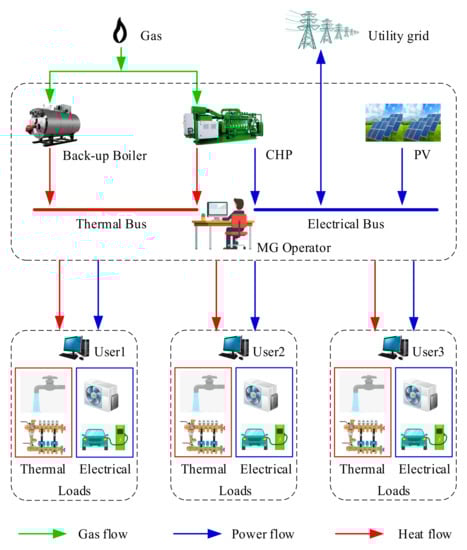
Figure 1.
System Framework.
As an energy consumer of MG, each user has a certain amount of thermal and electrical load. The electric load demand considered in this paper mainly consists of fixed electric load and shiftable electric load. Fixed electric load is used to guarantee the basic power demand of energy consumers, such as lighting, refrigerators, elevators, etc. Shiftable electric load is the load that consumers can regulate the operation time according to the dynamic electricity price and energy consumption benefits, such as air conditioning, dryers, electric vehicles, etc. The thermal demand considered in this paper mainly refers to the hot water and heating supply in winter, which is necessary to ensure the environmentally comfortable users’ temperature. Besides, users can reduce part of the thermal demand according to their adaptation to the indoor environment.
The energy transactions between the MGO and users are achieved by bargaining with each other. To maximize the operation benefit of the MGO, the supply of electric energy and heat energy will be determined according to the bargain prices. In addition, each user can bargain independently with the MGO and determine the energy consumption by shifting electric demand and reducing thermal demand.
3. Model of Energy Consumer
3.1. Model of Load Demand
The model of electric load demand is described as follows:
where , and are total electric load, fixed electric load, and shiftable electric load and of user in time slot, respectively. is the number of users, is the length of operation period. and are the lower limit and upper limit of shiftable electric load. is the feasible operation periods of shiftable electric load. is the sum of the electric load demand of user in the whole operation period.
The model of thermal demand is defined as follows:
where , and are the optimized thermal load, original thermal load, and cuttable thermal load of user in time slot . is the upper limit of .
3.2. Utility Model of Consumer
In this paper, Users can profit through electrical energy consumption rather than just pay for it. Especially for industrial and commercial prosumers, their profits increase with the growth of energy consumption []. Therefore, the user’s utility in the paper mainly considers the utility from energy consumption, the expenditure of buying electric/thermal energy, and the cost of comfortable dissatisfaction caused by reduced heat supply. And the objective function of user can be expressed as:
where, is the utility that user achieves from electrical energy consumption in time slot . is the preference parameter, which reflects the energy consumption characteristics of user . The larger means more willing users maximize profits through energy consumption. The logarithmic function has been widely used in the economics for modeling the behavior preferences of users, which is closely related to utility function and leads to proportionally fair DR []. and are the electrical bargaining price and electrical energy consumption between user and MGO, respectively. and are the thermal bargaining price and thermal energy consumption of user to MGO, respectively. is the cost factor of a comfortable temperature. According to the energy policies of some countries and cost constraints, and should be within a limited range
where and are the buying price and selling price of the power grid in time slot , respectively. and are the lower and upper limits of thermal price, respectively.
4. Model of MGO
4.1. Model of MT
An MT generator can provide electric and thermal energy for users through the natural gas drive. For MT generators with an output power of 20–500 kW, a niche market has emerged. Its energy conversion model can be described as:
where is the total energy of gas consumed by an MT, is the electrical efficiency of MT, and are the electrical energy and thermal energy of MT, respectively. is the heat loss efficiency of the waste heat recovery system, is the utilization efficiency of the heat supply system, is the heat-to-electric ratio of MT.
4.2. Model of Boiler
If the heat generated by an MT cannot meet the thermal load demand of users, the back-up boiler will be put into use, and the thermal energy generated by an MT can be expressed as follows
where is the total energy of gas consumed by the boiler, heat efficiency of the back-up boiler.
4.3. Utility Model of MGO
As the energy coordinator of the whole MG, the MGO needs to bargain with users about the heat price and the electricity price and then optimize the internal electricity and heat supply to maximize operation utility. The profit function of the MGO in each time slot can be formulated as follows:
In (13), is the benefit from trading with the power grid, is the revenue from selling electricity energy to the users, is the revenue from selling thermal energy to the users, is the cost of purchasing natural gas. In (14), and are the electricity energy selling to the power grid and the electricity energy buying from the power grid. In (17), is the low heating value of natural gas, is the natural gas selling price. The MGO needs to operate under an appropriate power level and price range, which consists of the following constraints:
where and are the maximum energy of gas consumed by MT and the maximum energy of gas consumed by Boiler. is the maximum net load of MG. Formula (20) is the constraint of the electric energy balance of MG, and is the generation power of PV arrays in a time slot . Formula (21) indicates the constraint of thermal energy balance in MG.
5. Nash Bargaining Game
In this section, the Nash bargaining theory is introduced to optimize the energy trading between the MGO and users. Additionally, the relationship between NBS and the social welfare maximization problem is studied.
5.1. Bargaining-Based Cooperation Model
The paper assumes that MGO and energy users who participated in energy bargaining are independent and rational. The premise of the MGO and users participating in energy bargaining is that they can improve their operational utilities by strategically choosing the volume and price of both electricity and heat, otherwise they will not participate in energy bargaining. Therefore, the following conditions need to be met:
where, and are respectively the utility of the MGO and user utility under original electrical and thermal prices. Thus, the bargaining-based optimal problem between the MGO and users can be realized by solving the following cooperative game optimization problem.
where is the benefit increment of MGO, and is the profit increment of user . and can de redefined as the disagreement points of the MGO and user , respectively. The constraints of variables {, , , , , } and constraints of variables {, , , } can be regarded as the strategy sets of the MGO and user , respectively. The equilibrium of bargaining can ensure that the benefits of cooperation are shared fairly by each stakeholder. Furthermore, according to the logarithm of the problem (25), the objective function can be further transformed into as follows:
By solving the NBS of (26), the following theorem is obtained.
Theorem 1.
The NBS of the bargaining problem (26) is also the solution to the social welfare maximum problem.
Proof.
Please see Appendix A. □
To illustrate the point, the social welfare maximization model is analyzed in the next subsection.
5.2. Social Welfare Maximization
As shown in (A9), the objective function of the social welfare maximization problem can be restated as:
From Theorem 1, the NBS can be achieved by solving (25) in a centralized approach, which requires the MGO collect all the DR information from end-users. However, the participants in the bargaining game usually only know the exchange bargaining information with each other. Besides, an important difference between function (26) and function (27) is that the trading information between the MGO and users is canceled out. Therefore, for the optimal energy trading problem, the Nash bargaining theory is necessary rather than simply using the social welfare maximization model. Furthermore, in the next section, a distributed algorithm is introduced to solve the NBS of the Nash bargaining problem with minimal information exchange between the MGO and users.
6. Distribution Solution
In this section, a distributed algorithm based on ADMM is proposed to solve the bargaining cooperative game between the MGO and users. The ADMM algorithm is widely used to solve the distributed optimization problem, which has been proved to have good convergence properties [].
6.1. Problem Decomposition
As mentioned above, the bargaining problem (26) involves variables of different participants. However, the variables , , , and couple the MGO and users together. It is not suitable for solving distributed optimization and needs to be decoupled. To achieve the NBS of the cooperative bargaining game, the MGO and users should reach a consensus on the volumes and prices of electrical and thermal energy. Therefore, the following auxiliary variables and constraints are introduced.
where and are the electrical bargaining price and electrical energy consumption of user to MGO, respectively. and are the thermal bargaining price and thermal energy consumption of user to MGO, respectively. and are the electrical bargaining price and electrical energy sales of MGO to user , respectively. and are the thermal bargaining price and thermal energy sale of MGO to user , respectively. In addition, the auxiliary variables , , and should satisfy the constraints of original variables , , and . Thus the problem (26) can be rewritten as:
The augmented Lagrangian functions for the distributed optimization objectives of MGO and users can be formulated as follows:
where, are the Lagrange multipliers of , are the Lagrange multipliers of , are the penalty coefficients.
6.2. Algorithm Implementation
As shown in (33) and (34), the information exchanges between MGO and users are limited. And it can be easily realized by many existing 1-to-N communication technologies. To achieve the NBS, the detailed implementation of distributed optimization algorithms for MGO and user is shown in Algorithms 1 and 2, respectively. In Algorithm 1, MGO can obtain the optimal solution {, , , , , } by solving the optimization problem in (33) according to the information collected from users. The variables {, , , } will be used to update dual variables , and then sent to corresponding users. In Algorithm 2, after receiving the updated variables {, , , } from MGO, each user solves the local optimization problem in (34) to achieve the optimal solution {, , , }, and then sends them to MGO. Based on the variables {, , , }, the dual variables will be updated in each iterative. In addition, both algorithms will be executed iteratively until the convergence condition is satisfied, which can be described as follows:
where is the convergence threshold of ADMM.
The specific implementation algorithm executed by MGO and user are as follows:
| Algorithm 1: Executed by MGO |
| 1: Initialized: = 0, , 2: repeat 3: (1) updated from users in receive buffer 4: (2) solve local optimal problem in (34) 5: (3) update dual variables 6: (4) send to corresponding users 7: (5) update iteraction index 8: until the convergence condition in (35) are satisfied 9: end |
| Algorithm 2: Executed by User |
| 1: Initialized: , , 2: repeat 3: (1) updated from MGO in receive buffer 4: (2) solve local optimal problem in (33) 5: (3) update dual variables send 6: (4) send to MGO 7: (5) update iteraction index 8: until the convergence condition in (35) are satisfied 9: end |
7. Case Study
To verify the effectiveness of the proposed Nash bargaining cooperative strategy, this paper uses the Yalmip tool with CPLEX to model and solve all the optimal problems under the MATLAB2016a compiler environment. The operation computer configuration is a 2.5 GHz Intel Core-i5 processor with16 GB of RAM and a 64-bit Windows 10 system.
7.1. Basic Data
In the paper, an MG comprised of three DRAs, a CHP system, and a PV generation system is selected as the study case. The data of heat load, electricity load, electricity prices, and photovoltaic are the measurement data of three commercial buildings provided by Hefei Thermal Power Group and Anhui Electric Power Co., Ltd. The time scale of data is hourly. The daily electricity demands of users and PV energy are shown in Figure 2, and the daily heat demands are shown in Figure 3. The adjustable proportion range of heat and electric load is set to 20%, respectively. Time-of-use (TOU) prices data for power grids are shown in Table 1. The price range of thermal energy is 0.15 RMB/kWh to 0.5 RMB/kWh, of which 0.15 RMB/kWh is the original thermal energy price. The price of natural gas is 2.33 RMB/m3, and the comfort coefficient of users 1, 2, and 3 are 0.04, 0.045, 0.05, respectively. The parameter is given according to the original load demand, as described in Appendix B. The parameters , , , , and are 300 kW, 100 kW, 0.4, 0.9, 0.05 and 0.95, respectively.
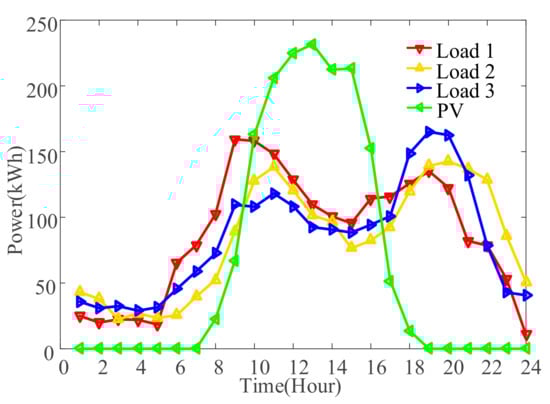
Figure 2.
PV and electric load demands.
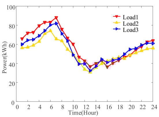
Figure 3.
Thermal load demands.

Table 1.
TOU prices of utility grid.
7.2. Trading Prices after Bargaining
The electricity trading prices after bargaining are shown in Figure 4, where the red, blue, and yellow solid lines represent the price information of user 1, user 2, and user 3, respectively. Obviously, all the trading prices are lower than the selling prices of the utility grid and higher than the utility grid’s buying prices. Therefore, end users can obtain more benefits from electric energy consumption.
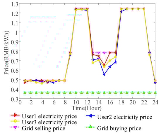
Figure 4.
Electricity trading prices after bargaining.
Figure 5 shows the heat trading prices of users. As depicted in Figure 5, the heat prices are all higher than the original (minimize) selling prices and lower than the maximum selling prices. Therefore, users will cut off parts of cuttable thermal demand to reduce unnecessary expenditure.
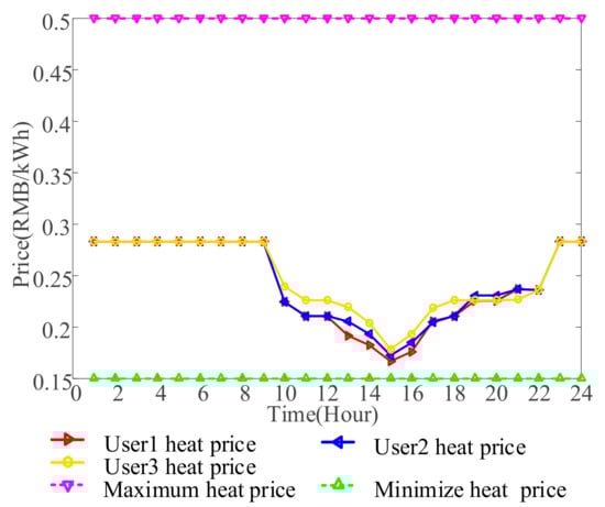
Figure 5.
Heat trading prices after bargaining.
7.3. Energy Consumption of Users
Users’ energy consumption strategies based on hybrid DR are shown in Figure 6a–c, respectively. To simplify the description, the energy consumption of user 1 in Figure 6a is taken as an example. Compared with the original electricity demand, the optimized demand decreases in time slots 9–12 and 18–21, mainly because the trading price in these two periods is close to the peak price. In 24 and 1–5 and 13–17 periods, the load demand increases because the trading prices in time slots 24 and 1–5 are close to valley prices, and the trading prices in time slots 13–17 are lower than the grid price. On the other hand, compared with the original thermal demand, the optimized heat demands are lower, indicating that the user can reduce the heat load demand according to the thermal price. Furthermore, as the thermal price in the 10–12 period is lower than that in other periods, users’ enthusiasm to participate in thermal DR is reduced, and thermal demand in these periods is lower.
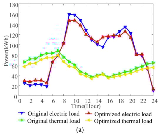
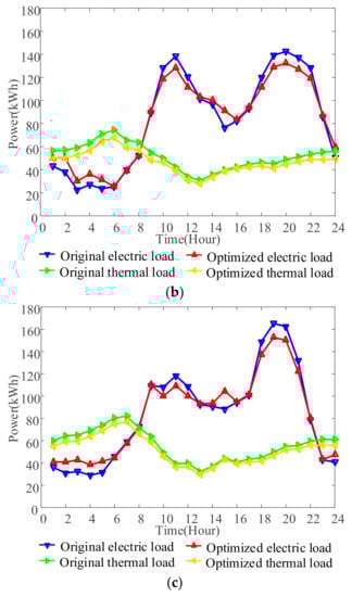
Figure 6.
Energy Consumption of Users. (a) User1. (b) User2. (c) User3.
7.4. Energy Supply Strategy of MGO
Figure 7 shows the energy supply strategy of the CHP system in both original and optimized situations. It is easy to see that the power of an MT reaches its maximum in time slots 1–10 and time slots 21–24. The main reason is that the thermal load demand in these two periods exceeds the maximum value of the MT’s heat supply. Additionally, to ensure the thermal energy supply to users, the standby boilers will be put into operation during these two periods. Compared with the original heat supply strategy, the optimized output power of the standby boiler is lower in these two periods. In time slots 11–20, as the demand for heat load during the day decreases, the standby boiler is no longer put into operation. The MT runs in the heat lead mode to supply heat energy for users. Under heat load DR, the optimized MT output power is lower than the original value. In addition, it can be seen that the electric energy supply of the MT varies with the thermal energy supply of the MT in all periods.
Figure 7.
Energy Supply of MT and Boiler.
To balance the electric energy in the MG, the MGO should trade with the utility grid. The optimized electricity net energy is shown in Figure 8. Compared with the original net profile, the optimized net profile is flatter. The electricity buying demands in time slots 10–12 and 18–21 are effectively suppressed. The redundant electric energy in time slots 1–5 and 13–15 has been well utilized. Therefore, the trading cost of the MGO is reduced.
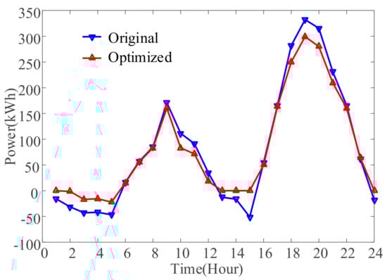
Figure 8.
Electricity trading between MGO and grid.
Figure 9 shows the decline in the MGO’s natural gas purchases from gas companies. Obviously, as thermal supply based on thermal DR decreases, the optimized gas purchasing volume decreases, thus reducing the gas consumption cost of the MGO.
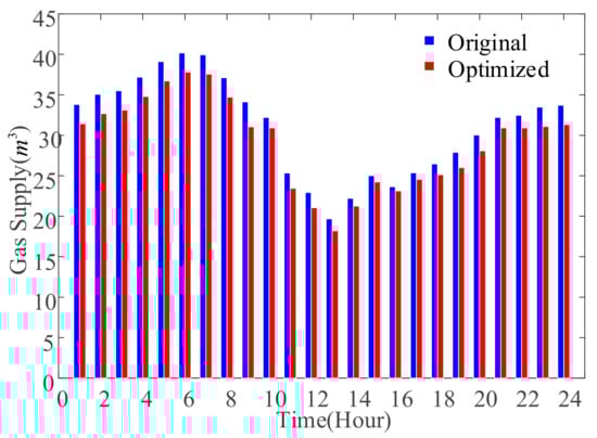
Figure 9.
Natural gas consumption.
7.5. Analysis of Economic Benefit
7.5.1. Compare with the Original Strategy
To further analyze the impact of the proposed model on economic benefits, the results of the comparison are shown in Table 2. The profit of the MGO is much higher when using the proposed strategy, which has a 5.15% profit increase compared with the original strategy. In addition, the profits of users 1–3 also increase 1.73%, 1.76%, and 1.78%, respectively.
Table 2.
Comparison of Economic utilities.
7.5.2. Compare with the Strategy Based on Stackelberg Game
As discussed in Section I, the study of [] mainly focuses on the optimization strategy based on the Stackelberg game. In the Stackelberg game, users determine energy consumption according to the prices specified by the MGO, while in the Nash cooperation game, the users decide their thermal and electric demand by bargaining with the MGO. To illustrate the advantage of the proposed strategy, the increased benefits of comparison are shown in Figure 10. Obviously, the MGO can gain more profits in the Stackelberg game, while users can get more benefits through the Nash bargaining game. However, as the essence of the Nash bargaining game is to maximize social welfare, all the participants in the MG can make more increased social benefits. Besides, the increased benefits are fairly distributed to the MGO and users. Therefore, the users are more willing to participate in the proposed energy trading strategy.
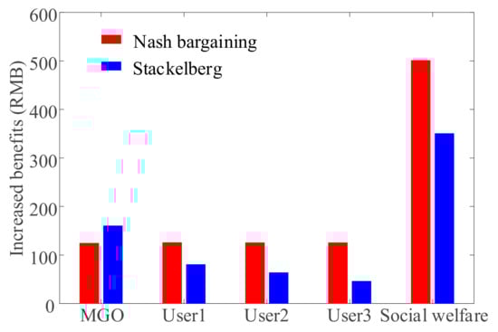
Figure 10.
Comparison of increased economic benefits.
8. Conclusions
In the present paper, an energy trading framework was proposed for CHP-MG with hybrid DR users, consisting of both electric and thermal demand. The energy trading between the MGO and users is modeled as a Nash bargaining game, where the MGO could maximize its operation profit by adjusting the energy supply of the CHP system and bargaining with users, and the user can determine the energy consumption of electricity and heat by bargaining with the MGO. Besides, the NBS of the proposed Nash bargaining game can maximize the social welfare of the whole MG system. Considering the bargaining information between the MGO and the user, a distributed algorithm based on ADMM is proposed to obtain the NBS. Finally, by using numerical studies, the numerical study shows that the proposed energy trading strategy can improve the social benefits for all participants by nearly 5.15%, and the profits of users 1–3 increase by 1.73%, 1.76%, and 1.78%, respectively.
Author Contributions
Conceptualization, C.Z. and C.B.Z.; methodology, C.Z.; software, C.Z.; validation, C.Z. and C.B.Z.; formal analysis, C.Z.; investigation, C.Z.; resources, C.Z.; data curation, C.Z.; writing—original draft preparation, C.Z.; writing—review and editing, C.Z.; visualization, C.Z.; supervision, C.B.Z.; project administration, C.B.Z.; funding acquisition, C.B.Z. All authors have read and agreed to the published version of the manuscript.
Funding
Collaborative Innovation Center of Industrial Energy-Saving and Power Quality Control, Anhui University (Nos.KFKT201904); Natural Science Research Project of Colleges and Universities of Anhui Provincial Department of Education (Nos.2020XJZR02); Domestic visiting program for outstanding young backbone teachers in Colleges and universities in Anhui Province (Nos. gxgnfx2021217); Key teaching research project of Anhui International Business Vocational College (Nos. 2020XM04); Teaching demonstration course of Anhui Provincial Department of Education (Nos. 2020SJJXSFK0529).
Institutional Review Board Statement
Not applicable.
Informed Consent Statement
Not applicable.
Data Availability Statement
Not applicable.
Conflicts of Interest
The authors declare no conflict of interest.
Appendix A
It is defined that
By substituting Formula (A5) into Formula (24), the problem (24) can be transformed into
The optimization problem in Formula (A2) can be solved in two steps.
(1) For a set of specific variables {, , , }, the optimal variable can be solved by setting the first derivative to zero.
Formula (A3) can be further transformed into:
Sum on both sides of the Equation (A4)
Therefore,
By Substituting Formula (A6) into Formula (A4), It can be obtained that
By substituting Formula (A6) and (A7) into (A2), the objective function (A2) can be reformulated as
The objective function (A8) can be equivalent to:
The objective function (A9) is composed of the transaction income of the power grid, the cost of natural gas, the benefit created by users through energy consumption, and the environmental dissatisfaction cost of users. Obviously, the essence of the objective function (A9) is the problem of maximizing social welfare. Therefore, the NBS of bargaining problem (26) is also the solution to the social welfare maximum problem.
Appendix B
The first derivative of problem (6) with respect to is calculated as:
By setting the right of (A10) to zero, the optimal value of can be solved as:
It is assumed that the original electric load is the optimal value of electric energy consumption under the grid selling price . Thus, parameter can be calculated as:
References
- Nižetić, S.; Djilali, N.; Papadopoulos, A.; Rodrigues, J.J. Smart technologies for promotion of energy effificiency, utilization of sustainable resources and waste management. J. Clean. Prod. 2019, 231, 565–591. [Google Scholar] [CrossRef]
- Basu, A.K.; Chowdhury, S.; Chowdhury, S.P. Impact of Strategic Deployment of CHP-Based DERs on Microgrid Reliability. IEEE Trans. Power Deliv. 2010, 25, 1697–1705. [Google Scholar] [CrossRef]
- Guan, X.; Zhang, H.; Xue, C. A method of selecting cold and heat sources for enterprises in an industrial park with combined cooling, heating, and power. J. Clean. Prod. 2018, 190, 608–617. [Google Scholar] [CrossRef]
- Vasilj, J.; Gros, S.; Jakus, D.; Zanon, M. Day-ahead scheduling and real-time Economic MPC of CHP unit in Microgrid with Smart buildings. IEEE Trans. Smart Grid 2017, 10, 1992–2001. [Google Scholar] [CrossRef]
- Lan, Y.; Guan, X.; Wu, J. Rollout strategies for real-time multi-energy scheduling in microgrid with storage system. IET Gener. Transm. Distrib. 2015, 10, 688–696. [Google Scholar] [CrossRef]
- Tang, J.; Ding, M.; Lu, S.; Li, S.; Huang, J.; Gu, W. Operational Flexibility Constrained Intraday Rolling Dispatch Strategy for CHP Microgrid. IEEE Access 2019, 7, 96639–96649. [Google Scholar] [CrossRef]
- Sohn, J.M. Generation Applications Package for Combined Heat Power in On-Grid and Off-Grid Microgrid Energy Management System. IEEE Access 2016, 4, 3444–3453. [Google Scholar] [CrossRef]
- Sun, T.; Lu, J.; Li, Z.; Lubkeman, D.L.; Lu, N. Modeling Combined Heat and Power Systems for Microgrid Applications. IEEE Trans. Smart Grid 2017, 9, 4172–4180. [Google Scholar] [CrossRef]
- Aghaei, J.; Alizadeh, M.I. Multi-objective self-scheduling of CHP (combined heat and power)-based microgrids considering demand response programs and ESSs (energy storage systems). Energy 2013, 55, 1044–1054. [Google Scholar] [CrossRef]
- Nazari-Heris, M.; Mohammadi-Ivatloo, B.; Gharehpetian, G.B.; Shahidehpour, M. Robust Short-Term Scheduling of Integrated Heat and Power Microgrids. IEEE Syst. J. 2018, 13, 3295–3303. [Google Scholar] [CrossRef]
- Liu, N.; He, L.; Yu, X.; Ma, L. Multi-Party Energy Management for Grid-Connected Microgrids with Heat and Electricity Coupled Demand Response. IEEE Trans. Ind. Inform. 2017, 14, 1887–1897. [Google Scholar] [CrossRef]
- Ma, L.; Liu, N.; Zhang, J.; Tushar, W.; Yuen, C. Energy Management for Joint Operation of CHP and PV Prosumers Inside a Grid-Connected Microgrid: A Game Theoretic Approach. IEEE Trans. Ind. Inform. 2016, 12, 1930–1941. [Google Scholar] [CrossRef]
- Alipour, M.; Mohammadi-Ivatloo, B.; Zare, K. Stochastic Scheduling of Renewable and CHP based Microgrids. IEEE Trans. Ind. Inform. 2015, 11, 1049–1058. [Google Scholar] [CrossRef]
- Fan, S.; Ai, Q.; Piao, L. Bargaining-based cooperative energy trading for distribution company and demand response. Appl. Energy 2018, 226, 469–482. [Google Scholar] [CrossRef]
- Albert, A.; Rajagopal, R. Finding the right consumers for thermal demand-response: An experimental evaluation. IEEE Trans. Smart Grid 2018, 9, 564–572. [Google Scholar] [CrossRef]
- Luo, X.; Lee, C.K.; Ng, W.M.; Yan, S.; Chaudhuri, B.; Hui, S.Y.R. Use of Adaptive Thermal Storage System as Smart Load for Voltage Control and Demand Response. IEEE Trans. Smart Grid 2016, 8, 1231–1241. [Google Scholar] [CrossRef]
- Liu, N.; Wang, J.; Wang, L. Hybrid Energy Sharing for Multiple Microgrids in an Integrated Heat-Electricity Energy System. IEEE Trans. Sustain. Energy 2018, 10, 1139–1151. [Google Scholar] [CrossRef]
- Liu, N.; Yu, X.; Wang, C.; Wang, J. Energy Sharing Management for Microgrids with PV Prosumers: A Stackelberg Game Approach. IEEE Trans. Ind. Inform. 2017, 13, 1088–1098. [Google Scholar] [CrossRef]
- Wu, C.; Gu, W.; Bo, R.; MehdipourPicha, H.; Jiang, P.; Wu, Z.; Lu, S.; Yao, S. Energy Trading and Generalized Nash Equilibrium in Combined Heat and Power Market. IEEE Trans. Power Syetems 2020, 35, 3378–3387. [Google Scholar] [CrossRef]
- Liu, N.; Zhou, L.; Wang, C.; Yu, X.; Ma, X. Heat-Electricity Coupled Peak Load Shifting for Multi-Energy Industrial Parks: A Stackelberg Game Approach. IEEE Trans. Sustain. Energy 2020, 11, 1858–1869. [Google Scholar] [CrossRef]
- Hong, M.; Luo, Z.Q.; Razaviyayn, M. Convergence Analysis of Alternating Direction Method of Multipliers for a Family of Nonconvex Problems. In Proceedings of the 2015 IEEE International Conference on Acoustics, Speech and Signal Processing, South Brisbane, QLD, Australia, 19–24 April 2015; pp. 3836–3840. [Google Scholar]
- Tushar, W.; Chai, B.; Yuen, C.; Smith, D.B.; Wood, K.L.; Yang, Z.; Poor, H.V. Three-Party Energy Management With Distributed Energy Resources in Smart Grid. IEEE Trans. Ind. Electron. 2015, 62, 2487–2498. [Google Scholar] [CrossRef] [Green Version]
Publisher’s Note: MDPI stays neutral with regard to jurisdictional claims in published maps and institutional affiliations. |
© 2022 by the authors. Licensee MDPI, Basel, Switzerland. This article is an open access article distributed under the terms and conditions of the Creative Commons Attribution (CC BY) license (https://creativecommons.org/licenses/by/4.0/).