Abstract
The accuracy of the Mueller polarimeter is usually affected by Gaussian–Poisson mixed noise, and by optimizing the instrument matrices of polarization state generator and polarization state analyzer in the measurement system, the estimation variance caused by Gaussian noise can be suppressed, and the estimation variance caused by Poisson noise can be made independent of the sample. However, the optimization procedure usually targets only the numerical value of the instrument matrix without considering how to configure the measurement system to achieve the optimal instrument matrix. In this paper, we investigate how to make the measurement system optimal for different measurement systems by combining geometric optimization on the Poincaré sphere and finally propose a series of measurement configurations for different applications.
1. Introduction
The polarization state of a beam of light can be represented by a Stokes vector, which is a four-dimensional vector, and the 4 × 4 transition matrix describing the change between different polarization states is called the Mueller matrix. The Mueller matrix can provide complete polarization properties of samples, which are related to their microstructural features [1]. Benefitting from this, a series of Mueller matrix imaging techniques have been developed for different applications, such as material characterization [2,3] and the microstructure of biological tissue measurement [4,5,6,7,8]. Among the available applications, measurement accuracy is always a top concern because precise Mueller matrix measurement can provide more detailed polarization features of samples.
The bedrock of Mueller matrix measurement is constructing a system of linear equations for the Mueller matrix elements by rationally setting the illumination and analysis polarization states. Therefore, the solution of the Mueller matrix depends on the matrix calculation process, in which the intensity error caused by Gaussian–Poisson mixed noise will be accumulated and amplificated [9]. In the design of the Mueller polarimeter, minimizing the estimation variance by choosing specific illumination and analysis polarization states, i.e., the instrument matrix of polarization state generator (PSG) and polarization state analyzer (PSA), has been extensively studied.
For the purposes of instrument matrix optimization, the determinant [10], condition number (CN) [10], and equally weighted variance (EWV) [11] indicators were proposed to find the optimal instrumentation matrices. These methods were successfully used to obtain the optimal configurations of polarimeters, including a rotatable retarder and a fixed polarizer-based Stokes polarimeter [11] and liquid-crystal variable retarders (LCVR)-based Mueller polarimeter [12] to reduce the estimation variance caused by additive Gaussian noise. However, the Poisson shot noise in the system cannot be ignored. The estimation variance due to Poisson noise should be not only minimal but also sample-independent. In this case, the optimal configuration of the system can only be optimized by EWV [13]. From another perspective, the optimal configuration of polarimeter can be given in terms of spherical t design. Foreman and Goudail proposed that when the system is in the presence of Gaussian noise and Poisson noise, the polyhedron formed by the polarization state corresponding to the instrument matrix on the Poincaré sphere should satisfy spherical 2 design and spherical 3 design, respectively [14,15]. In addition, appropriately expanding the dimensionality of the instrument matrices of PSG and PSA helps to further reduce the estimation variance [15].
Based on these methods, Mu et al. proposed a set of configurations of the Stokes polarimeter that can suppress both Gaussian and Poisson noise and reported the optimal measurement configurations for PSA, which consists of four analysis polarization states. The proposed configurations are by using a 142.1° wave plate and a 102.2° wave plate to produce two analysis polarization states, respectively, or using two quarter-wave plates [16]. However, waveplates with non-traditional retardance are not commonly used, and the PSG or PSA based on the rotating polarization elements will limit the application of polarimeters in some cases with high requirements on acquisition time.
In our previous study, we used a geometric optimization method based on Coulombic energy to optimize a rotating polarizer and rotating quarter-wave plate (RPRQ)-based PSG with a different number of illumination polarization states. This is combined with the dual division of a focal plane (DoFP) polarimeter [17,18] to build a Mueller matrix microscope capable of suppressing Gaussian–Poisson mixed noise [19]. Considering that DoFP cameras are not yet widely used, in this paper, we make the PSA have the same set of polarization analysis states as the set of PSG illumination states, which means the PSA also uses common devices such as waveplates or variable retarders followed by a standard camera; thus, we will not discuss these two parts separately.
To optimize the instrument matrix for the actual PSA or PSG, it is necessary to enable the PSA and PSG to produce arbitrary polarization states to generate arbitrary instrument matrices to meet the needs of optimal measurements. Moreover, considering different application scenarios, such as different requirements for cost, speed, and accuracy, we extend the previous work and summarize in detail the methods and steps for geometric optimization of measurement systems, and extend this method to a variety of PSAs and PSGs with different structures, including rotating polarizer and rotating quarter-wave plate (RPRQ), fixed polarizer followed by rotating half-wave plate and rotating quarter-wave plate (FPRHRQ) and fixed polarizer followed by dual full-wave variable retarders (FPDFVR); all of these can generate arbitrary polarization states.
In addition, this paper proposes a PSA and PSG based on a fixed polarizer followed by double half-wave variable retarders (FPDHVR). This system cannot satisfy the generation of arbitrary polarization states but can be optimized to achieve the optimal instrument matrix for four times illumination or four times analysis measurements in special cases.
2. Materials and Methods
2.1. Instrument Matrix Optimization Theory for Gaussian–Poisson Mixed Noise
EWV is the correct metric for polarimeters. Therefore, we used covariance analysis to quantify the effect of Gaussian or Poisson noise on the estimation variance of the Mueller matrix, and more details can be found in [9]. When additive Gaussian noise with the variance is present in the system, it follows that the estimation variance of the Mueller matrix that is caused by Gaussian noise CGaussian is:
where , denotes the Kronecker product, A and W are the instrument matrix of PSA and PSG, respectively and is the EWV of . Each column of W and A represents the Stokes vector corresponding to an illumination/analysis polarization state. It is clear that when the EWV of PSG and PSA are minimal, the estimation variance of the Gaussian noise is minimal as well.
For the Poisson noise in the system, using covariance analysis, the estimation variance that is caused by Poisson CPoisson noise in the system is [9]:
where is a 16-dimensional vector that consists of 16 elements of the Mueller matrix and is the kth element of . For the normalized Mueller matrix, its first term is always equal to 1. From the Equation (2), we can see that the first term is independent of the sample, and the second term is related to the last 15 Mueller matrix elements of the sample, which will lead to a consequent change in the estimation variance that is caused by Poisson noise as the sample changes. Fortunately, is a constant when the EWV of the instrument matrix of PSG and PSA is optimal. Therefore, the second term of CPoission is set to zero when the following equation is satisfied, thereby making the estimation variance caused by Poisson noise independent of the sample:
The equivalence condition of Equation (3) is: the sum of each row of W and A is zero [19]. When this condition is satisfied and the EWV of the instrument matrix of PSG and PSA is optimal, the estimation variance caused by Poisson noise is independent of the sample, and the estimation variance reaches the minimum value. At this time, the optimized CPoission can be expressed as:
To sum up, when the sum of each row of instrument matrices W and A is 0, and their EWV are optimal, the estimation variance caused by Gaussian–Poisson mixed noise is minimal and independent of the sample, and its minimum value is:
It is obvious that the sum of the last three rows in the measurement matrix is naturally zero when we divide the polarization states corresponding to the instrument matrix with N polarization illumination/analysis states into N/2 pairs of orthogonal polarization states [19]. The two polarization states symmetric about the center of the sphere are a pair of orthogonal polarization states on the Poincaré sphere. Therefore, if the polarization states corresponding to the instrument matrix form a polyhedron on the Poincaré sphere, where any polarization state has a polarization state symmetric about the center of the Poincaré sphere and the EWV of the instrument matrix is minimized, it must be the optimal instrument matrix. In this way, we can use the optimization method of geometric simplification to first constrain the polarization states corresponding to the instrument matrix so that each polarization state has a polarization state orthogonal to it. While doing so, the number of optimized parameters can be halved. Then, the genetic algorithm is used to find the minimum EWV to achieve the purpose of optimizing the instrument matrix.
It is worth noting that the above method can be used to optimize the optimal frame for N-dimensional instrument matrices (N is even), except for N = 4. For these optimal frames, both the sum of the estimation variance is optimal and the estimation variance of each Mueller matrix element is optimal, and independent of the sample [19]. For the case of N = 4, only two tetrahedrons with specific orientations have this property [9], the projections of these two tetrahedra at , , and planes are all squares. The instrument matrix corresponding to these two special tetrahedra is:
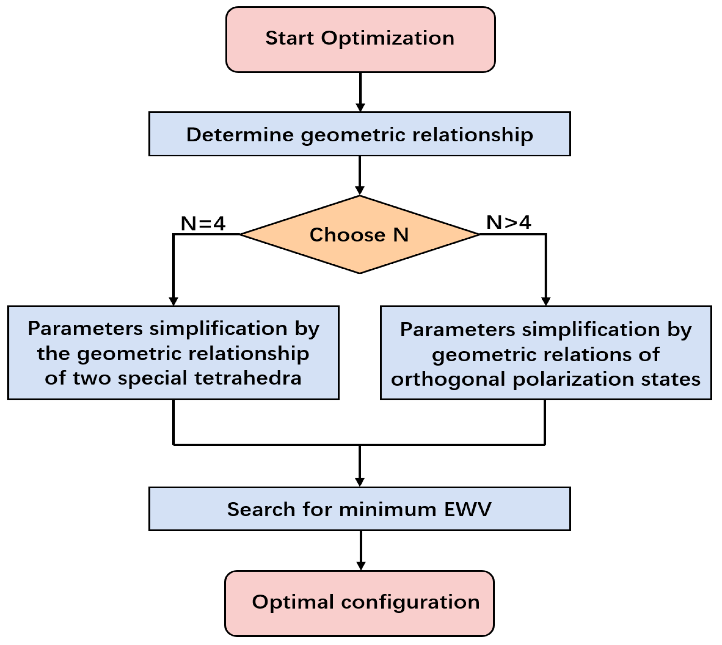
In summary, the optimization method for Gaussian–Poisson mixed noise that is proposed in this paper can be summarized as the following steps:
- (1)
- Determine the geometric relationship according to the selected system structure.
- (2)
- Choose the number N of illumination/analysis polarization states to be optimized.
- (3)
- If N = 4, the tetrahedron formed by the corresponding point of the illumination/analysis polarization states on the Poincaré sphere is constrained to be two tetrahedrons with special orientation in combination with the geometric relationship, so as to simplify the number of parameters that need to be optimized.
- (4)
- If N > 4, the corresponding points of the illumination/analysis polarization states on the Poincaré sphere are constrained to be pairs of orthogonal polarization states in combination with the geometric relationship, so as to simplify the number of parameters that need to be optimized.
- (5)
- The optimal configuration is obtained by searching the minimum EWV of the instrument matrix corresponding to the simplified parameters using the global optimization algorithm (i.e., genetic algorithm).
The optimization process is shown in Figure 1.
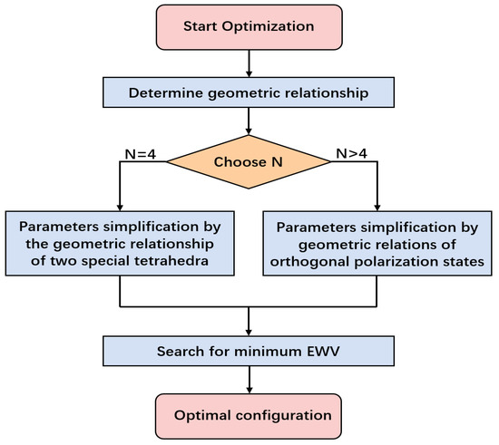
Figure 1.
Optimization process of proposed method.
2.2. Effect of Linear Retarders on Polarization States
The Poincaré sphere is a way to pictorially describe polarization states. Neglecting the first Stokes parameter , the three other Stokes parameters can be plotted directly in three-dimensional Cartesian coordinates. When we characterize the polarization states through the Poincaré sphere, any polarization state can be represented by a point on the surface of the Poincaré sphere. Besides, the instrument matrix is determined by multiple specific polarization states, so each instrument matrix can also be represented by a polyhedron composed of points on the surface of the Poincaré sphere. Then, the problem of how to optimize the instrument matrix of the PSG can be transformed into a geometric optimization problem of how to select N points on the Poincaré sphere.
Both PSA and PSG are composed of polarizers and retarders. In order to generate a special point on the surface of the Poincaré sphere, it is first necessary to figure out the effect of both polarizers and retarders on the polarization state on the Poincaré sphere. The Stokes parameters of a beam of light through a polarizer are easy to know, but retarders are unintuitive. The Mueller matrix of a retarder is
where is the angle of fast axis and is the retardance.
We can accurately calculate the polarization state of polarized light after passing through a retarder by the Mueller Matrix in Equation (7). However, if we need to generate a special polarization state, it will be complex to choose the incident polarization state or retarder’s angle and retardance. In addition, in order to make the polarization states satisfy certain geometric relationships, for example, the two states should be origin symmetry to each other on the Poincaré sphere when the illumination/analysis polarization states number is bigger than four, the first thing to figure out is how a retarder makes the polarization state on the Poincaré sphere change. Then, it will be easy to use the retarder to generate polarization states which we need to make them meet certain conditions.
2.2.1. Constant Fast Axis Angle and Variable Retardance
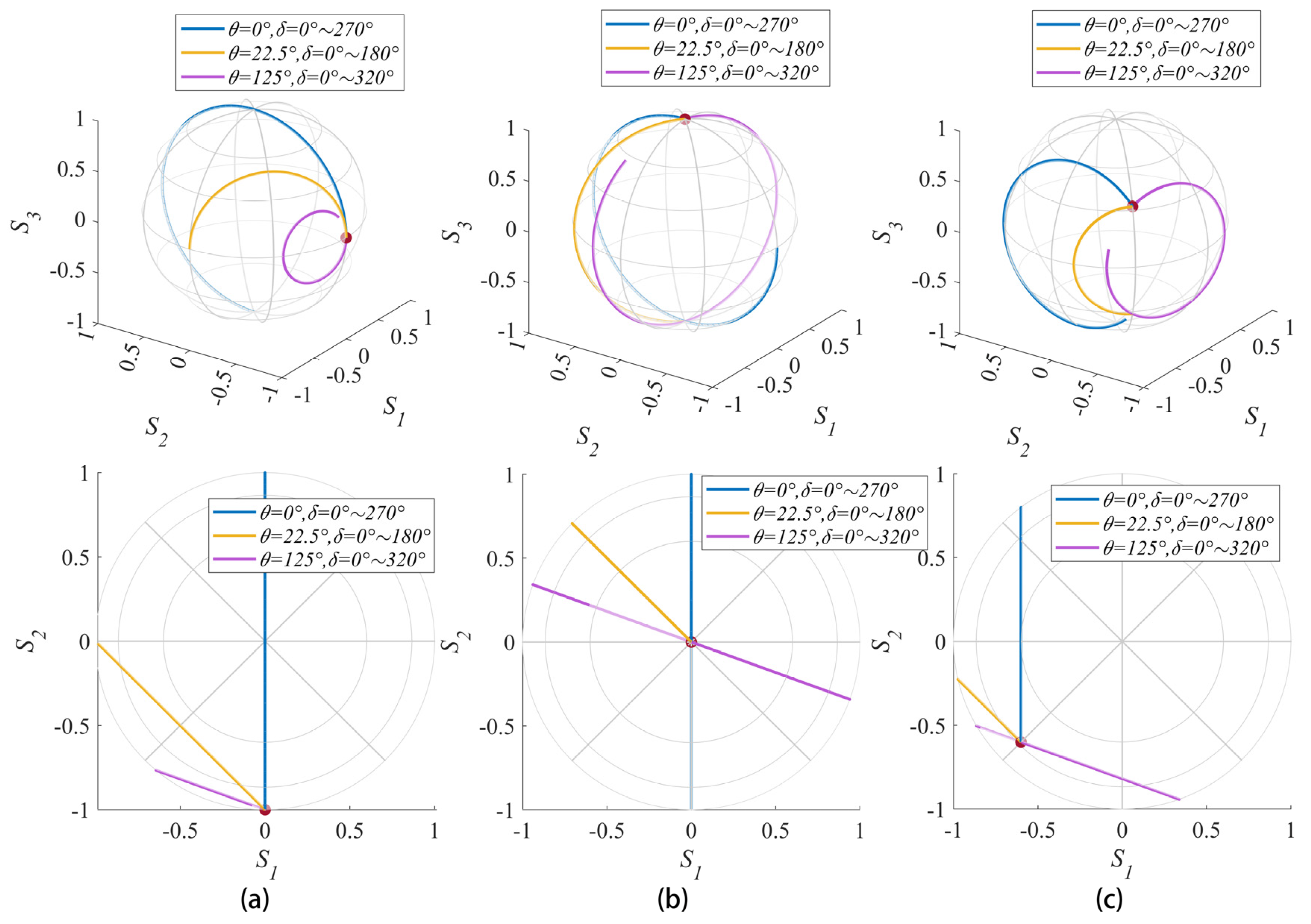
LCVR is typical of variable retarders. These retarders usually require a controlled cable connection, so they cannot change the fast axis angle during the measurement. Only when the measurement system is building, the variable retarder can change its angle. But the retardance of a variable retarder can be changed by the control cable. As shown in Figure 2, we selected three typical types of polarized light as incident light (linear polarization, circular polarization, and elliptical polarization), then calculated the polarization state by the Mueller matrix of retarders, and plotted the change of polarization state on the Poincaré sphere.
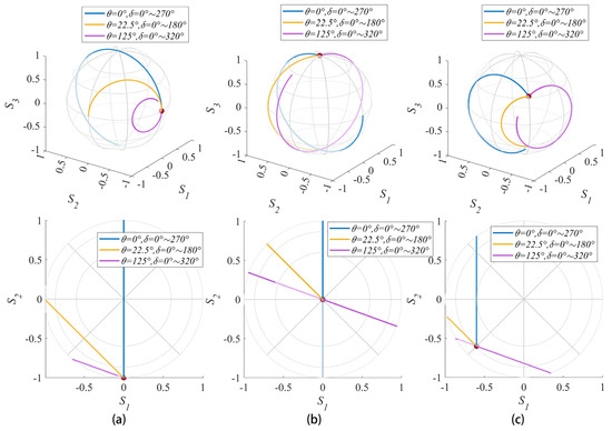
Figure 2.
The trajectory of several different incident light passes through a retarder with varying retardance. (a) Linear polarization, (b) Circular polarization, and (c) Elliptical polarization. Notice that all the trajectories appear as straight lines in the top view of the Poincaré sphere, and the lines’ directions are not changed with the incident light changing.
To show the general regulation of how variable retarders change the polarization states, we should have randomly selected their fast-axis angles and retardance, but to show them more clearly and to facilitate the reader’s understanding, we selected three special variable retarders with fixed fast-axis angles and retardance variation ranges: (a) the fast axis angle is 0° and the retardance changes between 0° to 270°; (b) the fast axis angle is 22.5° and the retardance changes between 0° to 180°; (c) the fast axis angle is 125° and the retardance changes between 0° to 320°.
From the top view of the Poincaré sphere, the trajectory of the polarization state changed on the Poincaré sphere will form a straight line in the projection of the plane. In addition, the angle of this projected straight line with the direction is . Note that the angle of the purple line in Figure 2a appears to be reversed from B and C. This is because the polarization state of the incident light in Figure 2a is a linear polarization, which makes the trajectory cross the hemisphere and form a reversal. Similarly, when the of the incident light Stokes vector is smaller than 0, it also makes the direction of trajectory look reversed. Therefore, when the fast axis angle is constant, the trajectory direction is also determined. Then, with the increase in the retardance, the trajectory will form an arc, and the radian of the arc is equal to retardance.
In this way, when the polarization state of incident light is known, we can easily generate the arbitrary polarization state we need through the variable retarder by first determining the directional relationship between the projection of the target polarization state and the current polarization state in the plane, thus determining the fast axis angle of the retarder. However, as mentioned before, the fast axis angle of the variable retarder cannot be changed easily, so we need two variable retarders to have orthogonal fast axis angles to each other (45° difference) to achieve the modulation of an arbitrary polarization state.
2.2.2. Constant Retardance and Variable Fast Axis Angle
Waveplates are one of the most common devices to change the polarization state and have constant retardance. Half-wave plate and quarter-wave plate are two common types of waveplates. The half-wave plate is usually used to shift the polarization direction of linearly polarized light, and the quarter-wave plate can be used to produce elliptical polarization or circular polarization. Besides, waveplates can be very easily fixed to rotating motors to change their fast axis angle. Different from the variable retarders, the retardance of a waveplate is constant, but the fast axis angle is variable.
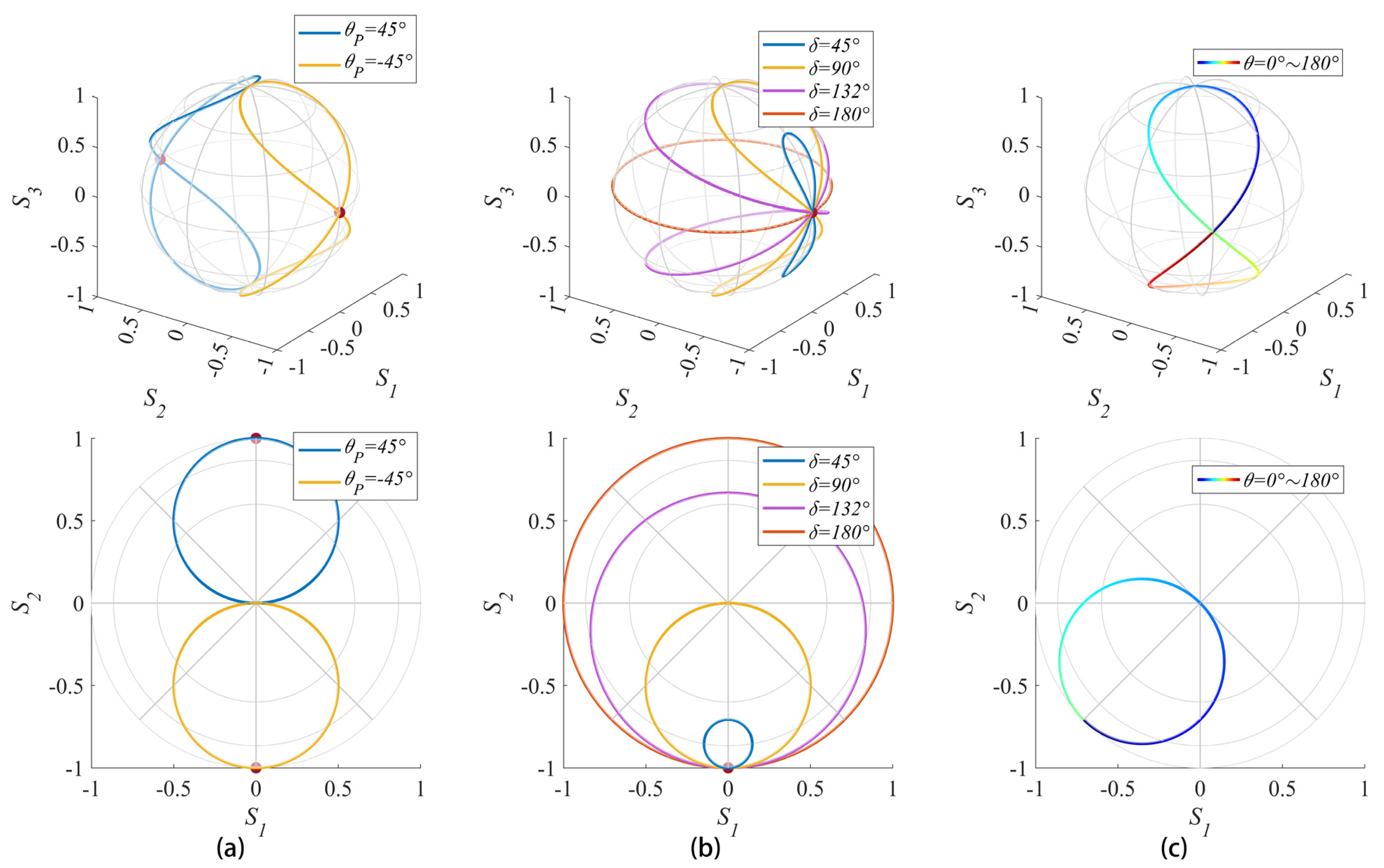
Similarly, we can calculate how the polarization state changed by the Mueller matrix of a retarder after a light beam traveled through it and plot the trajectory on the Poincaré sphere. As observed in Figure 3, we select a pair of orthogonal linearly polarized light as incident light and four waveplates with sequentially increasing retardance to demonstrate the changing of polarization states on the Poincaré sphere.
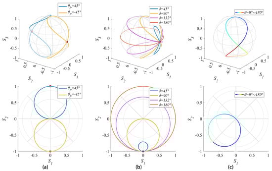
Figure 3.
The trajectories on the Poincaré sphere of polarized light passing through a rotating waveplate with (a) different incident polarized light generated by a polarizer with different angles, (b) different retardance, and (c) different fast axis angles. Notice that all the trajectories are 8-shaped curves, and with the incident polarized light changes, the curve’s position also changed.
If the incident polarized light is linearly polarized, the polarization state of the outgoing light will form an 8-shaped curve on the Poincaré sphere with the rotation of the waveplate. In addition, its projection in the plane is a circle whose diameter is determined by retardance. When the waveplate is a half-wave plate, the two segments of the 8-shaped curve coincide at the equator.
2.3. Multi Polarization Illumination/Analysis States (More Than Four)
2.3.1. A Rotating Polarizer Followed by a Rotating Quarter-Wave Plate
When we use the rotating waveplates to generate or analyze a polarization state, all the polarization states of the instrument matrix can only form an 8-shaped curve on the Poincaré sphere. However, if the polarization direction of the incident polarized light can be rotated, the 8-shaped curve will rotate along the equator of the Poincaré sphere so we can get any polarization state we need to optimize the instrument matrix. In our previous study, we used a PSG based on the rotating polarizer and rotating quarter-wave plate (RPRQ) to generate any polarization state and demonstrate the optimal configurations. Thus, we will first demonstrate the optimization method by the RPRQ measurement system.
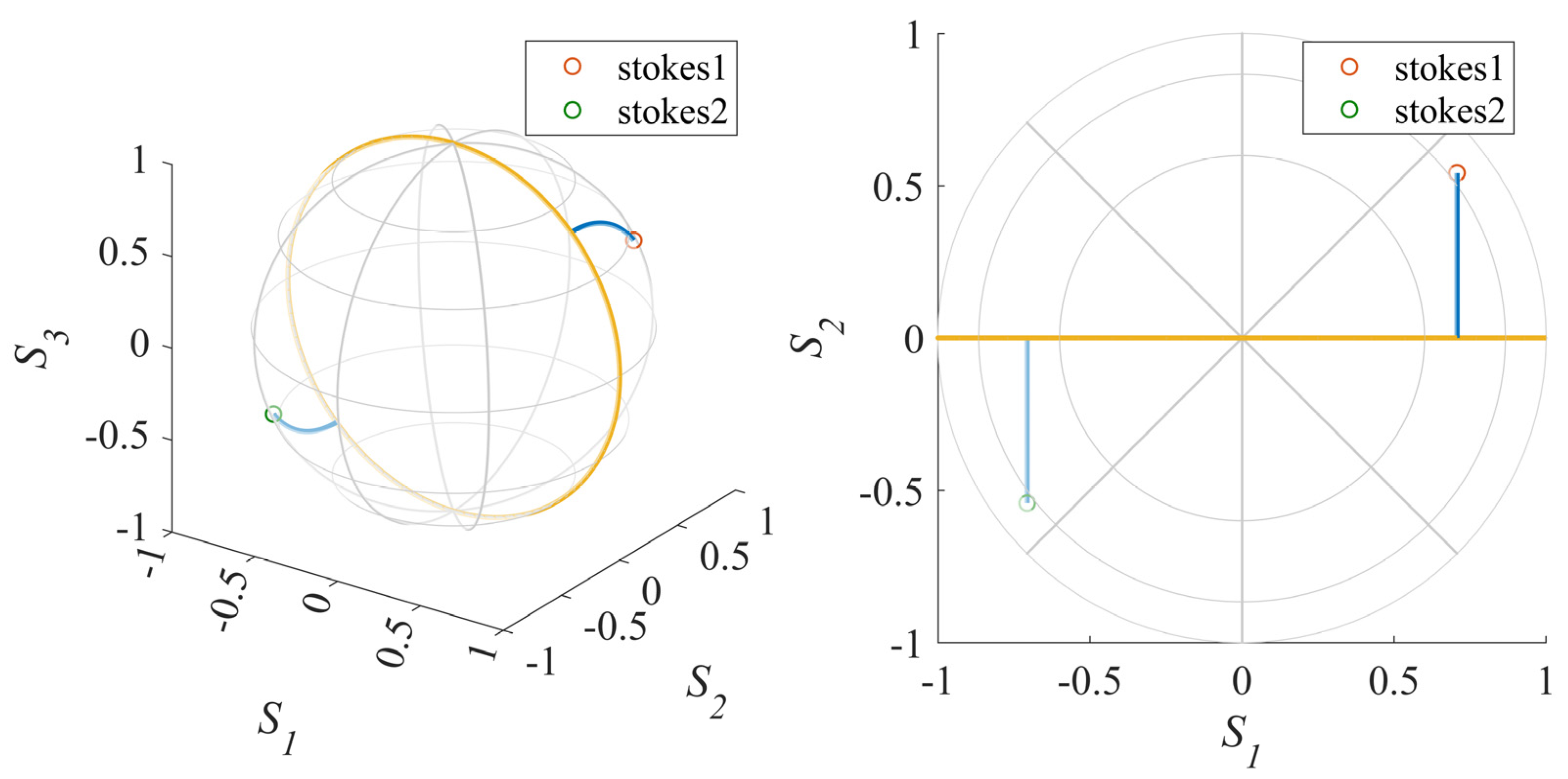
It is known that when the waveplate is rotating, the of its Stokes vector is only related to the angular difference between the waveplate fast axis angle and the polarizer transmission axis angle. In addition, the angle of the polarizer transmission axis determines the starting point of the 8-shaped curve on the Poincaré sphere; therefore, to generate a pair of orthogonal polarization states, the angles of the polarizer of two polarization states must be orthogonal to make the 8-shaped curve on the Poincaré sphere symmetrical:
After that, one polarization state is taken on each of the two 8-shaped curves, and makes sure that the of the two polarization states are opposite to each other. The position of the polarization state on the 8-shaped curve depends on the relative angle between the polarizer transmission axis angle and the waveplate fast axis angle. Therefore, the two relative angles should meet the relationship of 90 degrees difference:
where is the angle of polarizer transmission axis, is the angle of quarter-wave plate fast axis. When two polarization states are generated, if the configurations of and satisfy Equations (8) and (9), the geometric relationship of two polarization states on the Poincaré sphere is shown in Figure 4 and becomes orthogonal.
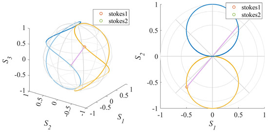
Figure 4.
A pair of orthogonal polarization states generated by rotating polarizer and rotating quart-wave plate. The two 8-shaped curves are 180 degrees apart.
Thus, to optimize an instrument matrix with a number of N polarization illumination/analysis states, the first step is obtaining N/2 pairs of orthogonal polarization states by Equations (8) and (9). Then, use the angles of the two rotating devices in the RPRQ as the optimized parameters to minimize the EWV of the final instrument matrix by means of genetic algorithms. This gives the actual configuration of and for 2/N pairs of orthogonal polarization states; then, the optimal configuration for N times polarization illumination/analysis states measurement is obtained based on the angular relationship between each pair of orthogonal polarization states.
However, the rotating polarizer requires the polarization state of the light source to be a unpolarized light as much as possible. Otherwise, it may lead to different light intensities in different polarization directions and make measurement errors. To avoid this problem, consider using an FPRHRQ measurement system to generate linearly polarized light in different directions. Then, to keep the pair of polarizer states orthogonal, the polarization directions of the initial linearly polarized light should remain unchanged, which means the half-wave plate angle should be the half of the polarizer angle. Then, the same method can be used to obtain the measurement configuration to make the EWV of the instrument matrix minimum. This also demonstrates that this method of optimization based on geometric constraint relations can be optimized for different PSG or PSA by modifying the constraints.
2.3.2. A Fixed Polarizer Followed by Dual Full-Wave Variable Retarders
When using the variable retarders to generate or analyze states, the design of the polarization state will be more intuitive. It can be considered as how to move a point on the Poincaré sphere to another point. According to the regularity demonstrated in Figure 2, the new polarization state can be reached by making the initial polarization state move on the surface of the Poincaré sphere along the target direction. The fast axis angle is half of the angle between the target direction and , and the retardance is equal to the radian between the initial and target polarization states. However, the angle of the fast axis of the variable retarder cannot be freely changed during the actual measurement, so we chose to use two orthogonal variable retarders to generate the target polarization state, and the angle between the fast axis of the first retarder and the polarizer is also orthogonal (45°). When the angle of the polarizer is 0°, of the Stokes vector is changed by the first retarder and is changed by the second retarder. This makes it very easy to generate arbitrary polarization states and determine measurement configurations. However, as long as the orthogonality of the angle is satisfied, other angles are also workable, but this paper will take the angles (0°, 45°, 0°) as an example.
For two polarization states that are orthogonal to each other, each component of their Stokes vectors is opposite (except ), and in this measurement system, and are determined separately by the two variable retarders, so the retardance of the first retarder should be made to differ by 180° between the two illumination/analysis measurements:
However, limited by the fast-axis angle, the polarization states are orthogonal but do not freely generate arbitrary polarization states. Therefore, a second variable retarder is needed for further modulation. When the retardance of the second variable retarder satisfies:
where and are the retardance of two retarders. Then, the polarization states will be orthogonal, as shown in Figure 5.
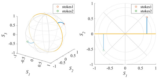
Figure 5.
A pair of orthogonal polarization states by variable retarder. The start points of two blue curves are 180 degrees apart and the length of blue curves are same.
Then, use a similar approach as Section 2.3.1, find the specific configuration of N/2 pairs of and when EWV is smallest. Finally, obtain specific configurations for N times polarization illumination/analysis states measurement by Equations (10) and (11). The measurement configuration obtained in this way satisfies the optimal instrument matrix and is optimized for both Poisson noise and Gaussian noise.
2.4. Four Polarization Illumination/Analysis States
When performing a four-polarization illumination/analysis states measurement, if the geometric constraint is still targeted by generating two pairs of orthogonal polarization states, the final instrument matrix will form a plane on the Poincaré sphere, at which point the CN of the instrument matrix will be infinite. Such an instrument matrix does not enable the measurement of the Muller matrix. In fact, there are only two optimal instrument matrices, as shown in Equation (6):
These two instrument matrices form exactly one regular tetrahedron on the Poincaré sphere, and three orthographic projections are square. If the instrument matrix is only optimized by making the EWV minimum, it can only be sure that the final instrument matrix is a regular tetrahedron, but cannot limit the direction of it. It is obviously not the optimal instrument matrix given in Equation (6). The instrument matrix is only optimized for Gaussian noise but cannot make the estimation variance caused by Poisson noise independent and minimum. Thus, it is necessary to perform geometric constraints to make the instrument matrix optimal. In addition, depending on the measurement system, suitable constraints can be chosen to facilitate the implementation of the actual measurement configuration. Moreover, the geometric constraint will no longer be conducted in a pair of orthogonal states, but by the properties of the regular tetrahedron.
2.4.1. A Rotating Polarizer Followed by a Rotating Quarter-Wave Plate
Likely, we optimize the optimal configuration of the RPRQ measurement system by geometric constraint.
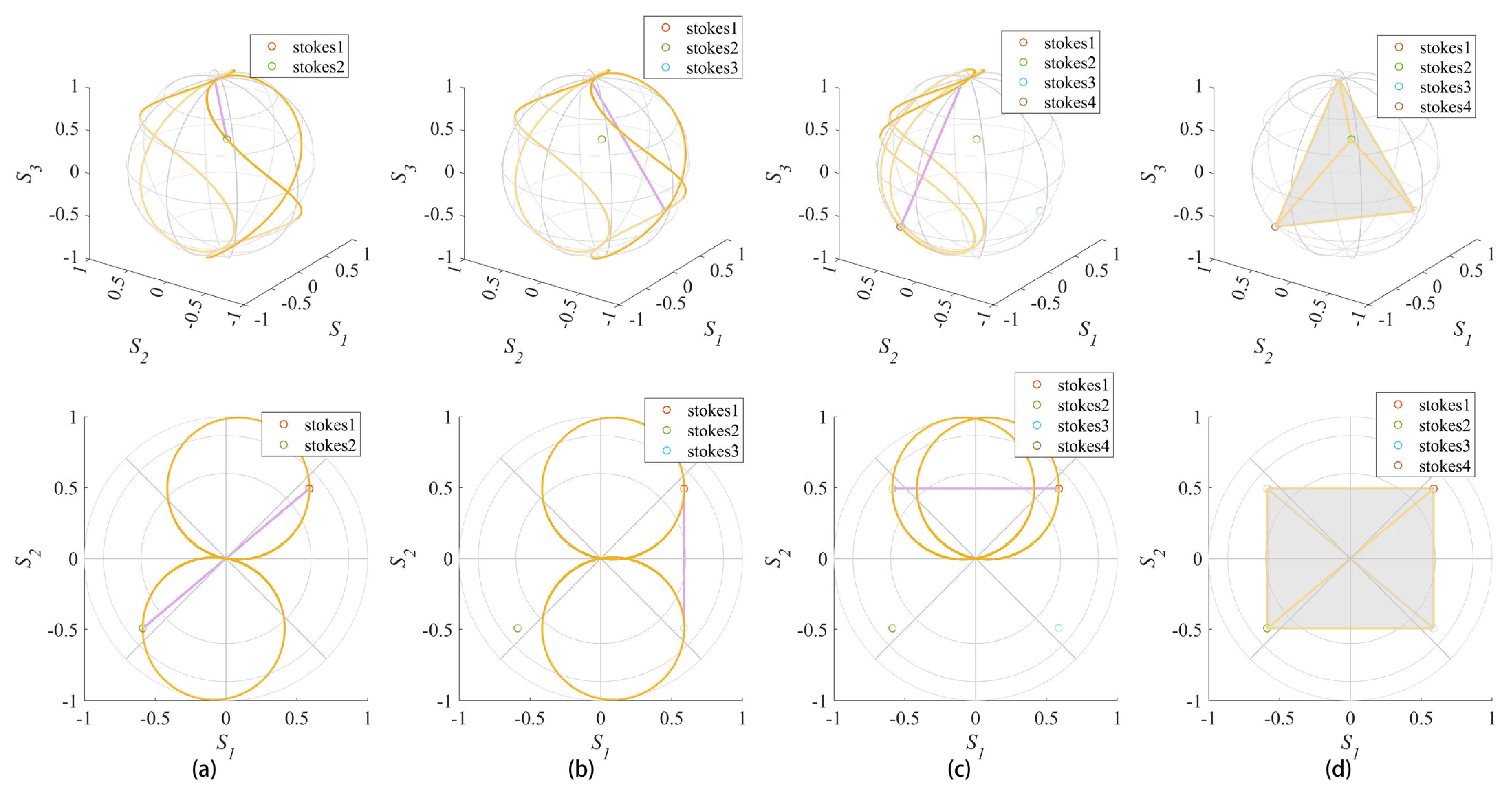
To make the final instrument matrix optimal, we first consider making three orthographic projections of the tetrahedron formed by the instrument matrix on the Poincaré sphere rectangular. The three polarization states are constrained to satisfy certain geometric relations with an arbitrary polarization state on the Poincaré sphere. The four polarization states are denoted as stokes1, stokes2, stokes3, and stokes4, as shown in Figure 6.
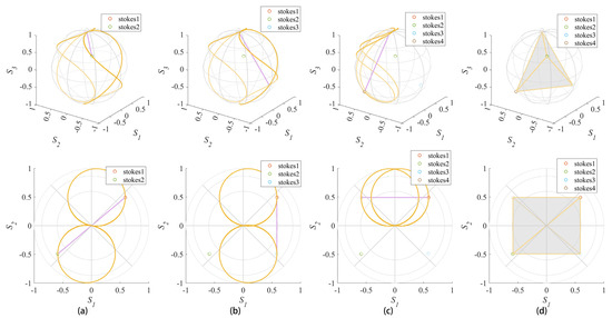
Figure 6.
The geometric relationship between the polarization states after constraint. Respectively, the geometric relationships between (a) stokes2 and stokes1, (b) stokes3 and stokes1, and (c) stokes4 and stokes1. (d) is the tetrahedron formed by the four polarization states on the Poincaré sphere.
The of stokes1 and stokes2 should be equal and the , of stokes1 and stokes2 should be opposite. This means stokes2 is the point on the Poincaré sphere where stokes1 has rotated 180° along the latitude. Therefore, if the position of the polarization state on the 8-shaped curve generated by the rotating waveplate is fixed during two measurements, and the two 8-shaped curves are orthogonal, two polarization states will satisfy this geometric relationship. Combined with the effect of the waveplate on the polarization state, the configuration of these two measurements should satisfy:
Since the polarizer is rotated by 90° to make the 8-shaped curve orthogonality, the fast axis angle of the quart-wave plate needs to be rotated by 90° to keep the relative angle between the quart-wave plate and the polarizer constant.
Then, the of stokes1 and stokes3 should be equal and the , of stokes1 and stokes3 should be opposite. The two 8-shaped curves are symmetrical about the plane, and the relative positions on the 8-shaped curve should complement each other. Thus, the geometric constraints are:
The geometric relationship between stokes4 and stokes1 is like the relationship between stokes3 and stokes1. The only difference is that the two 8-shaped curves are symmetrical about the plane. Therefore, similarly, their geometric constraints are:
where , , , are the angles of polarizer and , , , are the angles of quart-wave plate. With those geometric constraints, the three orthographic projections of the tetrahedron that formed by the four polarization states on the Poincaré sphere are all rectangular. Then, find and of the first illumination/analysis state to make the EWV of the final instrument matrix minimal by genetic algorithm, and the optimal configuration can be determined.
In addition, the rotating polarizer can also be replaced by a rotating half-wave plate followed a fixed polarizer. Then, the geometric constraints of the polarizer angle will change to the half-wave plate angle. However, the angle is half of the polarizer angle.
2.4.2. A Fixed Polarizer Followed by DUAL Full-Wave Variable Retarders
When optimizing a four-polarization illumination/analysis states measurement configuration with two variable retarders, we still do the geometric constraints by making the tetrahedron’s three orthographic projections rectangular. In addition, because how polarization states on the Poincaré sphere changed by variable retarder is easy to know, the constraints are also clear.
Since there are no rotating devices in the measurement system and the polarizer and retarders are fixed during the measurement, the angle of each of them needs to be determined first. As in Section 2.3.2, to ensure that arbitrary polarization states can be generated and to facilitate geometric optimization, the angle of the polarizer is fixed to 0°, and the angles of retarders are fixed to 45° and 0°, respectively.
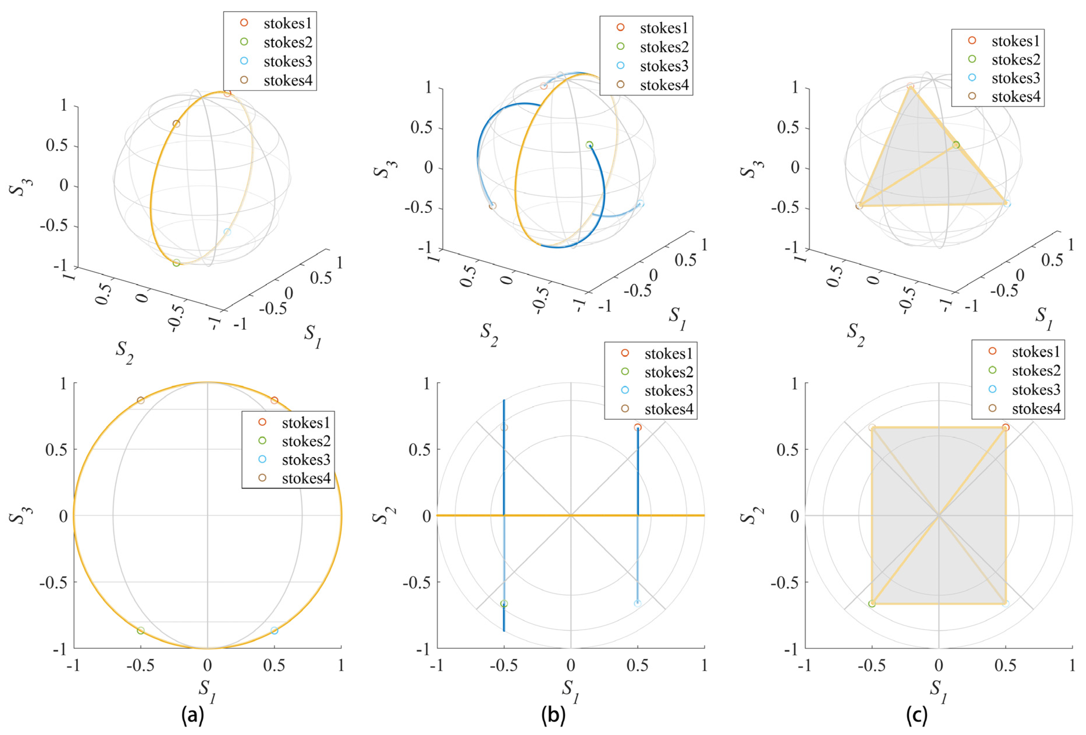
By varying the retardance of the first retarder, the absolute values of of the four polarization states stokes vectors are equal and distributed in the four quadrants. In addition, the four polarization states are denoted as stokes1, stokes2, stokes3, and stokes4, as shown in Figure 7. Stokes1 is an arbitrary polarization state and the geometric constraints are satisfied by the difference in the retardance between the other three polarization states and stokes1:
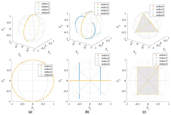
Figure 7.
The geometric relationship between the polarization states after constraint. (a) is the relationship by the first retarder and (b) is the relationship by two retarders. (c) is the tetrahedron formed by the four polarization states on the Poincaré sphere, and its top view is rectangle.
On this basis, we divided stokes1 and stokes3 into one group and stokes2 and stokes4 into another group. As long as the retardance of the second retarder is made equal for each group of measurements and, at the same time, the retardance of the two groups are complementary, the four polarization states on the Poincaré sphere will form a tetrahedron as shown in Figure 7c. The constraints are:
Then, find and of the first illumination/analysis state to make the EWV of the final instrument matrix minimal by genetic algorithm. This will make the tetrahedron become a regular tetrahedron and the instrument matrix will be the same as one of Equation (6), which is the optimal instrument matrix. At the same time, the measurement configuration can also be known by the constraints after the and is known.
2.4.3. A Fixed Polarizer Followed by Dual Half-Wave Variable Retarders
Whether the rotating quart-wave plates followed a rotating polarizer or two full-wave variable retarders followed a fixed polarizer measurement system can generate every polarization state to make it possible to generate arbitrary instrument matrices. If using two half-wave variable retarders followed a fixed polarizer as the measurement system, when the angles of the polarizer and retarders are orthogonal as 2.3.2, it can only generate half the polarization states on the Poincaré sphere at most. All the polarization states that can be generated will form a hemisphere on the surface of the Poincaré sphere. It will not be able to make the polarization states uniformly distributed on the Poincaré sphere and obtain the optimal instrument matrix.
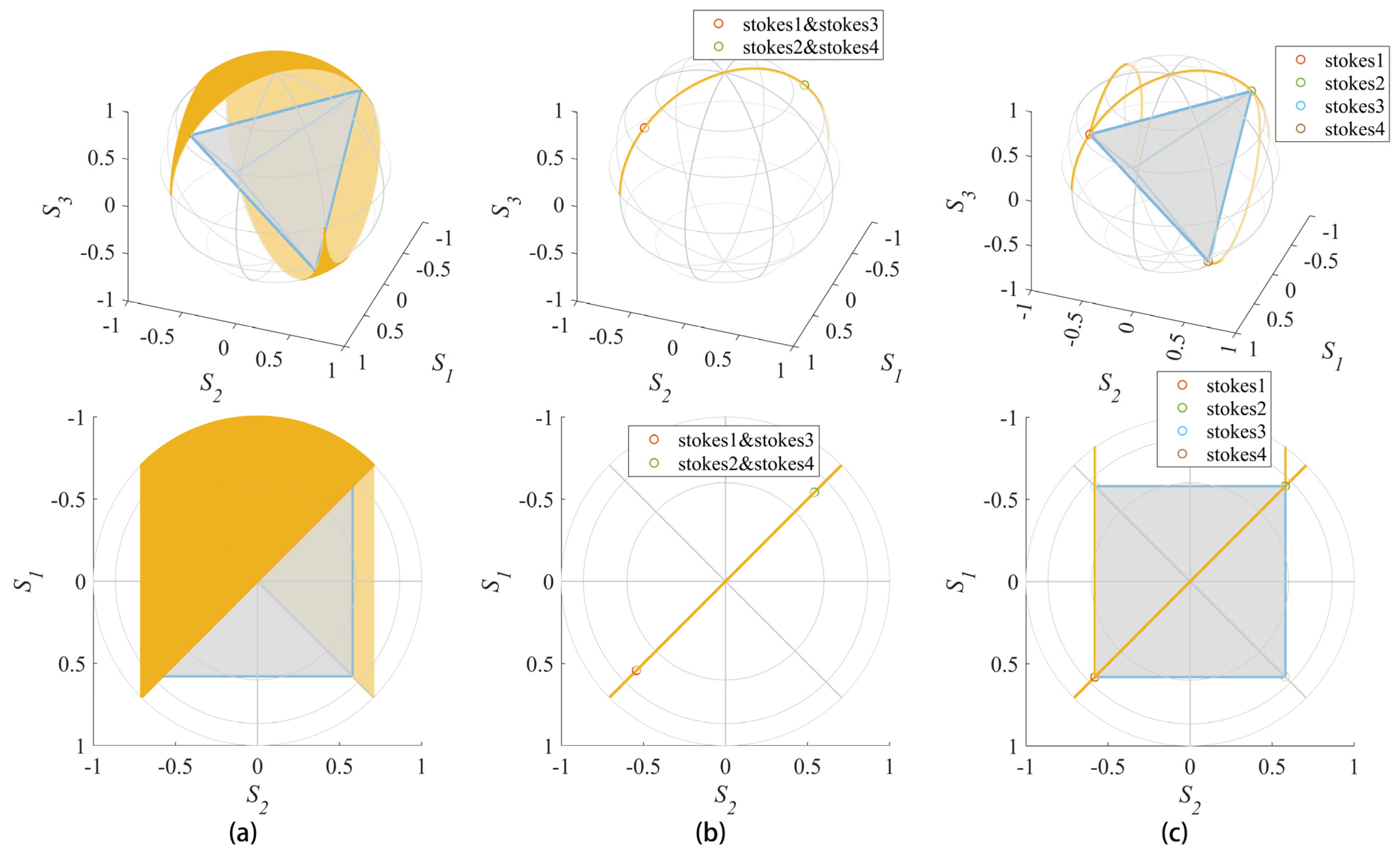
It can be noted that the top view of the regular tetrahedron formed by the optimal instrument matrix in Equation (6) is a square whose diagonals are just past the origin and along 45° and 135°. If the angles of the polarizer and the two delays are −22.5°, 22.5°, and 45° respectively, the possible generated polarization states will include the arcs where the two diagonals are located as shown in Figure 8a.
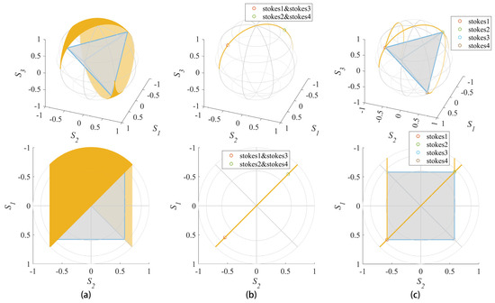
Figure 8.
(a) shows the optimal instrument matrix and all possible generated polarization states. (b) is the polarization states geometric relationships by the first retarder and (c) shows the relationships by two retarders. All the four states are at the edge of the surface.
The four polarization states are divided into two groups, one for stokes1 and stokes3 and one for stokes2 and stokes4. When changing the polarization states by the first retarder, make the two retardance of each group equal. It will make the two points coincide on the Poincaré sphere. In addition, the two retardance of the two groups should complement each other. Thus, the constraints of the first retarder are:
Then, the retardance of the second retarder is made to be 0° and 180° for two measurements in each group, respectively:
where and are the retardance of the two half-wave variable retarders.
After all the constraints, three orthographic projections of the tetrahedron formed by the instrument matrix on the Poincaré sphere will be rectangle and the top view will be square. Then, the value of can be calculated either by genetic algorithm or directly to make the instrument matrix reach the optimum. This configuration makes the retardance of the second half-wave variable retarder to be 0° and 180°, making maximum use of its retardance range.
However, since there are two optimal instrument matrices for four polarization illumination/analysis states measurements, only one of them can be achieved with this configuration. However, when both the polarizer and the retarders are rotated 45° in the same direction, another optimal instrument matrix can be achieved.
3. Results
The actual measurement configurations after geometry optimization and minimum EWV optimization are given in this section. Although the minimum EWV of the measurement system instrument matrix decreases as the number of polarization illumination/analysis states increase, this section will only give the optimal configuration at 4 and 8 states, considering that measuring too many states would be time-consuming.
Complete configurations will be given in the Supplementary Materials. In addition, we calculated the EWV and CN of the optimized instrument matrix for each set of measurement system configurations. All these given measurement configurations are optimal configurations, and the instrument matrix of the measurement system with this configuration will be the optimal instrument matrix.
In Table 1, Table 2, Table 3 and Table 4, two configurations are given for the four polarization illumination/analysis states, which are two different optimal instrument matrices, while only one configuration is given as an example for the eight polarization illumination/analysis states. It is important to note that several different optimal configurations can be obtained by the optimization method proposed in this paper, and there is never only one solution; these optimal configurations are all equivalent, so only one configuration is given as an example. In addition, the angle of the polarizer and the angle of the retarders is not unique in all variable retarder measurement systems, and the angle proposed in this paper is the most convenient one for analysis and implementation.

Table 1.
The optimal measurement configurations of RPRQ.
Table 2.
The optimal measurement configurations of FPRHRQ.
Table 3.
The optimal measurement configurations of FPDFVR.
Table 4.
The optimal measurement configurations of FPDHVR.
4. Discussion
Since polarization measurement requires the generation and analysis of polarization states by PSA and PSG, and the polarization state analysis is based on the measurement of different polarization states projections, the selection of the generated polarization states and the projected target polarization states is a very important issue, which greatly affects the accuracy of the measurement system and the noise feature. The optimization of the instrument matrix is usually mostly performed by complex algebraic calculations, which require huge arithmetic power, and the complexity of the optimization grows exponentially with the number of polarization illumination/analysis states. For example, in the work of Mu et al. [16], a cost function is built to account for the Euclidian distance between the columns (in the original paper this is rows, because the definition of the instrument matrix is transposed to each other) of the measurement matrix and the columns of the ideal matrix:
Then, minimize the cost function by changing retardance and azimuth to approximate the optimal instrument matrix and obtain the optimal configuration. Each polarization state has a and needed to be optimal, which means there are eight variables needed to be optimal. However, in our method, there will only be one or two (depending on the measurement structure) variables to optimize. However, the cost function proposed by Mu et al. is the Euclidian distance between the columns of the measurement matrix and the columns of the ideal matrix, which means the ideal matrix must be known, or the optimal matrix should be optimized before the configuration optimization. However, only the ideal matrix of four polarization illumination/analysis states is known as Equation (6) shows; therefore, this method cannot optimize the measurement system with more than four polarization illumination/analysis states.
By analyzing the Gaussian–Poisson mixed noise, the optimization problem of the instrument matrix can be reduced to two main indicators—a zero row sum and a minimum EWV of the instrument matrix. Then, change the first indicator into a geometric constraint to make it easy to meet the indicator. Furthermore, instead of simply optimizing the instrument matrix, we propose several different measurement systems and optimize configurations of the measurement systems in order to make the optimization results practically meaningful. In the optimization process, we analyze in detail how different measurement systems make geometric simplification to reduce the complexity of the optimization and obtain the optimal instrument matrix.
We finally obtained the optimal configurations for a number of different measurement systems represented by RPRQ, FPRHRQ, FPDFVR, and FPDHVR. As can be observed from Table 1, Table 2, Table 3 and Table 4, the instrument matrixes optimized by this method have minimal CN and EWV. When performing polarization measurements, if these measurement systems that we have optimized are used, the given measurement configurations can be directly used to make the measurements optimal without complicated optimization of the instrument matrix.
Although only a single PSA or PSG is optimized in this paper, the PSA and PSG have the same set of polarization states in illumination and analysis, and they can both be directly used in the best configuration given. When performing polarization measurements, the optimal Stokes measurement can be achieved by using a PSA with this configuration, or the optimal configuration can be applied to both PSA and PSG to make the whole Müller measurement system optimal and effectively restrain noise, improve measurement accuracy, and make the estimation variance caused by Poisson noise independent of the sample.
In contrast to instrument matrix optimization methods such as minimizing CN [10] and EWV [11], this method optimizes the actual measurement configuration rather than just the instrument matrix itself, and the method can be applied to measurement systems with different devices. If the measurement system used is not mentioned in this paper, the optimization method can also be used. Thus, we could obtain the optimal measurement configuration with the regular measurement structure and make it possible to use the optimal configuration for measurement.
However, this method still has some weaknesses and limitations. First, it can only optimize for the even number of polarization illumination/analysis states. What is more, the sum of the instrument matrix rows must be zero after the geometric constraint, but the geometric constraint is only a special case to make the sum zero. This means that this method cannot be optimized for all cases.
However, the optimal instrument matrix is not unique, but there are an infinite number of them (the instrument matrix of more than four polarization illumination/analysis states). The optimal instrument matrix optimized by this method is also not unique. Each time this method is used for optimization, different results may be obtained. This difference may affect the speed of the measurement. For example, the rotating motor rotates at different angles. This is also a potentially optimizable factor.
5. Conclusions
In this paper, we present an optimization method based on geometric simplification for obtaining the optimal instrument matrix of PSG/PSA in Mueller polarimetry. This method can be used to optimize different measurement structures and obtain the optimal measurement configuration for common Mueller polarimetry. The configuration can minimize the estimation variance caused by both Gaussian and Poison noise and can be directly used in the measurement and have practical significance. The results can be used as a practical manual when performing Mueller polarimetry.
Supplementary Materials
The following supporting information can be downloaded at: www.mdpi.com/article/10.3390/app12136521/s1, Table S1: The complete optimal measurement configurations of RPRQ; Table S2: The complete optimal measurement configurations of FPRHRQ; Table S3: The complete optimal measurement configurations of FPDFVR.
Author Contributions
Conceptualization, Q.Z.; methodology, Z.H.; software, Q.Z. and Z.H.; formal analysis, Z.H.; resources, H.M.; writing—original draft preparation, Z.H. and Q.Z.; writing—review and editing, Z.H., Q.Z. and H.M.; supervision, H.M.; project administration, H.M.; funding acquisition, H.M. All authors have read and agreed to the published version of the manuscript.
Funding
This research was funded by the Guangdong Development Project of Science and Technology, grant number 2020B1111040001 and the National Science Foundation of China, grant number 11974206.
Institutional Review Board Statement
Not applicable.
Informed Consent Statement
Not applicable.
Data Availability Statement
Not applicable.
Conflicts of Interest
The authors declare no conflict of interest.
References
- He, C.; He, H.; Chang, J.; Chen, B.; Ma, H.; Booth, M.J. Polarisation optics for biomedical and clinical applications: A review. Light Sci. Appl. 2021, 10, 194. [Google Scholar] [CrossRef] [PubMed]
- Gödecke, M.L.; Frenner, K.; Osten, W. Model-based characterisation of complex periodic nanostructures by white-light Mueller-matrix Fourier scatterometry. Light Adv. Manuf. 2021, 2, 237–250. [Google Scholar] [CrossRef]
- Chen, C.; Chen, X.; Wang, C.; Sheng, S.; Song, L.; Gu, H.; Liu, S. Imaging Mueller matrix ellipsometry with sub-micron resolution based on back focal plane scanning. Opt. Express 2021, 29, 32712–32727. [Google Scholar] [CrossRef] [PubMed]
- Tuchin, V.V. Polarized light interaction with tissues. J. Biomed. Opt. 2016, 21, 071114. [Google Scholar] [CrossRef] [PubMed] [Green Version]
- Dong, Y.; Wan, J.; Wang, X.; Xue, J.-H.; Zou, J.; He, H.; Li, P.; Hou, A.; Ma, H. A Polarization-Imaging-Based Machine Learning Framework for Quantitative Pathological Diagnosis of Cervical Precancerous Lesions. IEEE Trans. Med. Imaging 2021, 40, 3728–3738. [Google Scholar] [CrossRef] [PubMed]
- Schucht, P.; Lee, H.R.; Mezouar, H.M.; Hewer, E.; Raabe, A.; Murek, M.; Zubak, I.; Goldberg, J.; Kövari, E.; Pierangelo, A. Visualization of white matter fiber tracts of brain tissue sections with wide-field imaging Mueller polarimetry. IEEE Trans. Med. Imaging 2020, 39, 4376–4382. [Google Scholar] [CrossRef] [PubMed]
- He, C.; Chang, J.; Salter, P.S.; Shen, Y.; Dai, B.; Li, P.; Jin, Y.; Thodika, S.C.; Li, M.; Tariq, A. Revealing complex optical phenomena through vectorial metrics. Adv. Photonics 2022, 4, 026001. [Google Scholar] [CrossRef]
- Ghosh, N.; Vitkin, A.I. Tissue polarimetry: Concepts, challenges, applications, and outlook. J. Biomed. Opt. 2011, 16, 110801. [Google Scholar] [CrossRef] [PubMed] [Green Version]
- Anna, G.; Goudail, F. Optimal Mueller matrix estimation in the presence of Poisson shot noise. Opt. Express 2012, 20, 21331–21340. [Google Scholar] [CrossRef] [PubMed]
- Ambirajan, A.; Look, D. Optimum angles for a polarimeter: Part I. Opt. Eng. 1995, 34, 1651–1655. [Google Scholar] [CrossRef]
- Sabatke, D.; Descour, M.; Dereniak, E.; Sweatt, W.; Kemme, S.; Phipps, G. Optimization of retardance for a complete Stokes polarimeter. Opt. Lett. 2000, 25, 802–804. [Google Scholar] [CrossRef] [PubMed] [Green Version]
- De Martino, A.; Kim, Y.-K.; Garcia-Caurel, E.; Laude, B.; Drévillon, B. Optimized Mueller polarimeter with liquid crystals. Opt. Lett. 2003, 28, 616–618. [Google Scholar] [CrossRef] [PubMed]
- Foreman, M.R.; Goudail, F. On the equivalence of optimization metrics in Stokes polarimetry. Opt. Eng. 2019, 58, 082410. [Google Scholar] [CrossRef]
- Foreman, M.R.; Favaro, A.; Aiello, A. Optimal frames for polarization state reconstruction. Phys. Rev. Lett. 2015, 115, 263901. [Google Scholar] [CrossRef] [PubMed] [Green Version]
- Goudail, F. Optimal Mueller matrix estimation in the presence of additive and Poisson noise for any number of illumination and analysis states. Opt. Lett. 2017, 42, 2153–2156. [Google Scholar] [CrossRef] [PubMed]
- Mu, T.; Chen, Z.; Zhang, C.; Liang, R. Optimal configurations of full-Stokes polarimeter with immunity to both Poisson and Gaussian noise. J. Opt. 2016, 18, 055702. [Google Scholar] [CrossRef]
- Roussel, S.; Boffety, M.; Goudail, F. On the optimal ways to perform full Stokes measurements with a linear division-of-focal-plane polarimetric imager and a retarder. Opt. Lett. 2019, 44, 2927–2930. [Google Scholar] [CrossRef]
- Huang, T.; Meng, R.; Qi, J.; Liu, Y.; Wang, X.; Chen, Y.; Liao, R.; Ma, H. Fast Mueller matrix microscope based on dual DoFP polarimeters. Opt. Lett. 2021, 46, 1676–1679. [Google Scholar] [CrossRef] [PubMed]
- Zhao, Q.; Huang, T.; Hu, Z.; Bu, T.; Liu, S.; Liao, R.; Ma, H. Geometric optimization method for a polarization state generator of a Mueller matrix microscope. Opt. Lett. 2021, 46, 5631–5634. [Google Scholar] [CrossRef] [PubMed]

Publisher’s Note: MDPI stays neutral with regard to jurisdictional claims in published maps and institutional affiliations. |
© 2022 by the authors. Licensee MDPI, Basel, Switzerland. This article is an open access article distributed under the terms and conditions of the Creative Commons Attribution (CC BY) license (https://creativecommons.org/licenses/by/4.0/).