Abstract
Time series prediction is crucial for advanced control and management of complex systems, while the actual data are usually highly nonlinear and nonstationary. A novel broad echo state network is proposed herein for the prediction problem of complex time series data. Firstly, the framework of the broad echo state network with cascade of mapping nodes (CMBESN) is designed by embedding the echo state network units into the broad learning system. Secondly, the number of enhancement layer nodes of the CMBESN is determined by proposing an incremental algorithm. It can obtain the optimal network structure parameters. Meanwhile, an optimization method is proposed based on the nonstationary statistic metrics to determine the enhancement layer. Finally, experiments are conducted both on the simulated and actual datasets. The results show that the proposed CMBESN and its optimization have good prediction capability for nonstationary time series data.
1. Introduction
Time series data are generated in various fields such as social sciences [1], meteorological industry [2,3], financial market [4], modern agriculture [5,6], electric power field [7], etc. Especially in the Big Data and IoT industry [8], it is essential to analyze the regular patterns of time series data and predict the trends for system management and control. Time series prediction can help to sense and control the systems in advance. However, the time-series data in all systems are often highly nonlinear, nonstationary, and massive [9], making it very difficult to predict trends accurately. Therefore, the prediction of complex time series data has become a hot research topic in data mining [10].
Scholars have explored different methods for the nonlinear and nonstationary problems in time series data prediction. The existing prediction methods are mainly classified into statistical methods [11,12], shallow machine learning methods [13,14], deep learning methods [15,16], and broad learning methods [17,18]. The main statistical prediction methods are the autoregression model (AR), moving average model (MA), autoregression moving average model (ARMA), and differential auto regression integrated moving average model (ARIMA). The methods above mainly transform the nonstationary time series into the stationary time series by variance or integration. It is difficult to reduce the loss function value with stable data transformation, so it is unsuitable for practical applications. Deep learning methods develop from external neural networks. Deep learning forms a vertically deepened network structure, which improves the network’s learning ability. However, the time and computational costs are high since all layers need the training simultaneously. Meanwhile, the gradient disappearance and explosion can occur in deep learning. The broad learning method is proposed for the resource occupation problem of deep learning. A broad learning system (BLS) [19] is built with a horizontal extension instead of a vertical deepening. It achieves feature extraction ability through a mapping layer and an enhancement layer. It dramatically reduces the time cost, but it is found that the prediction accuracy of time series needs improving in practice. It has been the main issue to utilize and improve the machine learning methods for accurate time series prediction.
The literature research and previous experiments found that an effective prediction model often depends on the network structure and the computation resource occupation. The BLS has advantages in terms of resource occupation but has limited capability in data regression. A lightweight network of echo state network (ESN) was found in the previous study, which is computationally fast and has a strong nonlinear fitting ability. For the prediction problem of complex time-series data, this paper designs a new broad echo state network to utilize the advantages of different neural networks fully. The new network takes the BLS with mapping layer cascade as the basic framework and combines the broad structure with the ESN. An optimization method is also proposed for the enhancement layer to improve the prediction ability.
This paper is organized as follows. Section 2 introduces the related methods for time series prediction. Section 3 introduces the proposed broad echo state network and the optimization method based on an incremental algorithm and nonstationary metrics. Section 4 presents the experimental results and analysis of the model application. Section 5 presents a summary and discussion of the method.
2. Related Works
2.1. Time Series Prediction Methods
In this section, several classical time series prediction methods are introduced, some of which will be set as the experimental comparison models. The existing time series prediction methods include statistical and machine learning methods.
The early statistical methods are mainly the AR [20], MA [21], and ARMA [22] models based on the randomness theory. They use the regression equation established by the historical and current data correlation. The ARMA model solves the problem of random variation terms, widely used in the early prediction of nonstationary time series. With the development of computer technology, machine learning, and deep learning have been applied for time series prediction. The external neural networks can solve the simple classification problems, which face the weak performance in the time series regression. Then deep learning and BLS develop from external neural networks. The classical deep learning methods for the time series prediction are GRU [23], LSTM [24], DeepESN [25], graph neural network [26], Fusion network [27], etc. LSTM belongs to the RNN network [28] and mainly solves the problem of gradient disappearance and explosion in RNN [29]. GRU is a variant of LSTM that combines the forget gate and output gate into one update gate. It has a more concise structure than LSTM. DeepESN is a network that connects multiple reservoir units in the deep learning idea. It realizes a multi-layer reserve pool, which improves the network stability and prediction ability to a certain extent. The BLS realizes the horizontal expansion rather than a vertical deepening of deep networks. The BLS can significantly reduce the training time and the complex structure [30]. The BLS based on the cascade of mapping layer (CMBLS) [19] is a variant structure of the width learning network, which aims to enhance the extraction of data features and improve the performance of the network model.
As mentioned above, statistical methods for the prediction problem can analyze the stable and linear time series data. Their performance will degrade when the time series is nonstationary and nonlinear. Then the machine learning methods are applied for the complex time series regression. Machine learning relies mainly on the data characteristics, the network structure, and computation resources. The ESN and DeepESN have been the emerging models in the recurrent networks with a lightweight training mode. The BLS is proposed to reduce the network scale of the deep learning networks. There is no ideal network to cover the strong learning ability and appropriate structure [31]. Then we try to propose a new model which combines the BLS and ESN to take advantage of different networks. The new network is studied to balance the model learning ability and the computation resource occupancy.
2.2. Broad Learning System
The BLS is a forward neural network based on the connection of random vector functions. Its network structure is divided into a mapping layer, reinforcement layer, and output layer, as shown in Figure 1. Compared with the random vector function connectivity network, the mapping layer replaces the output layer. The BLS can update the network structure quickly by adding nodes in the mapping and enhancement layers, which benefits from the efficient incremental algorithm. The BLS extracts the mapping features of the original data by feeding the input data into the mapping layer and then uses the output of the mapping layer as the input of the enhancement layer. It can achieve the data feature and finally obtains the output weight matrix by the ridge regression method.
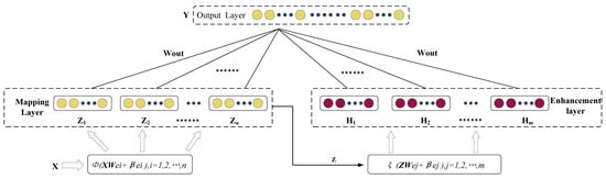
Figure 1.
The network structure of BLS [19].
The structure of the BLS can be flexibly changed, and the CMBLS is a typical variant. The network of CMBLS is shown in Figure 2. CMBLS cascades each node of the mapping layer in turn. It maps the original input data as the first mapping node through the mapping function. Then the output of the first mapping node is used as the second mapping node input. It continues to form the structure of the mapping layer cascade, which achieves sparse and nonlinear mapping of data features [32]. It can weaken the correlation between adjacent features and improve the transformation of low-level to high-level features.
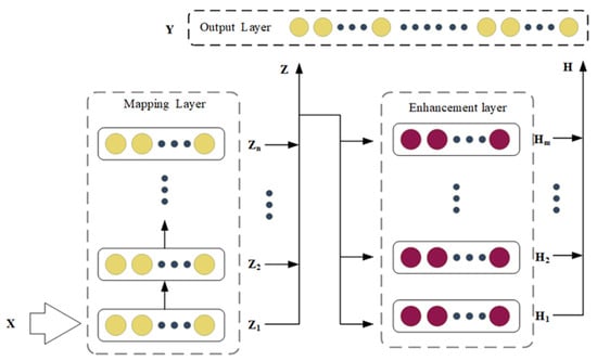
Figure 2.
The network structure of CMBLS [33].
As a basis of the proposed method in this paper, the CMBLS is introduced first. As shown in Figure 2, the mapping layer node is defined as , the enhancement layer node is defined as , and the input data sequence is . The first node of the mapping layer is .
where are the randomly initialized weight matrix and bias vector, respectively, is the mapping function, are similar to in that they are generated through a random initialization mechanism. The second mapping node is defined as:
By the same analogy, the mapping layer node is defined as:
where is the randomly initialized weight matrix and bias vector, and the input of the enhancement layer node is the input of the mapping layer node, so the enhancement layer node is defined as:
where is randomly initialized, is the excitation function, the enhancement layer node is defined as , and the combined matrix of the enhancement and mapping layers is , so the output and the output weight matrix of CMBLS are defined as:
where denotes the regularization factor, which takes the value range (0,1), denotes the transpose, and represents the unit matrix. is found by the pseudo-inverse method.
2.3. Echo State Network
The ESN follows the concept of reservoir computation which is very suitable for modeling complex nonlinear relationships. The ESN contains an input, reservoir, and output layer. The original data are mapped to the high-latitude reserve pool through the input layer, and the model is trained through the pool computation structure. The ESN differs from other network models in terms of training mechanisms. Firstly, there is no error backpropagation in the ESN. Secondly, the ESN need not train the input weight matrix and hidden layer weight matrix. Only the output weight matrix needs to be trained [34]. The network structure of the ESN is shown in Figure 3.
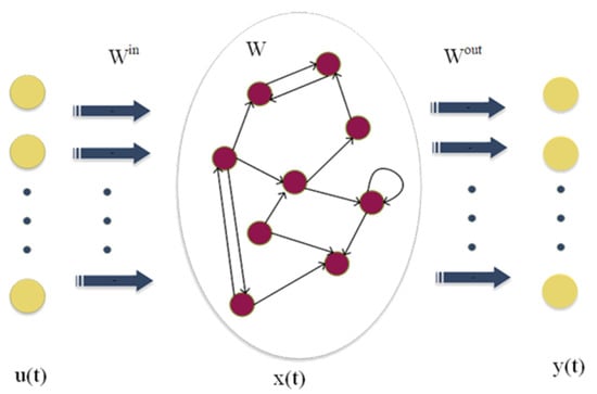
Figure 3.
ESN model structure [35].
As shown in Figure 3, the input layer of ESN at the time is defined as , the reservoir state is , and the network output is , where represents the number of input samples, the number of reservoir neurons, and the output dimension in that order.
To ensure the echo state property of the ESN, the spectral radius range is usually set to (0,1), and the update and output formulas of the reservoir are shown below.
denotes the state of the reservoir at the time , denotes the network output at the time , denotes the leakage coefficient, denotes the weight matrix generated by the random initialization of the input layer and the reservoir, respectively, denotes the activation function of the reservoir and the output layer. Formula (7) can continuously update the state of the ESN model after each set of data input to the model until all data input is completed and the output of the network model is obtained by Formula (8). Where is calculated as follows:
denotes the state matrix of the reservoir pool, means the actual output, λ denotes the regularization coefficient, denotes the unit matrix, and is computed by many methods, including ridge regression [36], recursive least squares [37], singular value decomposition, and pseudo-inverse solution [38], etc. The training mechanism of the ESN network can be simply training the output weight matrix, which will significantly reduce the difficulty of network training.
As a clear comparison, the methods of time series prediction above are summarized as follows in Table 1, including the statistical approach, classical deep learning network, and broad learning system.

Table 1.
Description of each model.
As shown in Table 1, each model has different characteristics and deficiencies. For the DeepESN in the deep learning networks, the echo state structure brings a new approach to regression modeling. The BLS can reduce the training resources in the typical deep learning networks. Analyzing related works above can provide a solution to combine the different advantages. Then an improved method is proposed in this paper. The new network takes the BLS as the basic framework and integrates the broad structure with the ESN. It is improved both on the learning ability and the network structure scale.
3. Novel Broad Echo State Network
3.1. Network Based on the Cascade of Mapping Nodes
As mentioned in Section 2.2, CMBLS develops from BLS. In CMBLS, the original data are mapped to the first mapping nodes, the first layer’s output is set as the input of the second layer, and so on. The improved structure of CMBLS can strengthen the feature extraction ability. It is theoretically proved that CMBLS retains a good fitting function [19]. The mapping nodes and enhancement layers in both BLS and CMBLS are essential for a reliable regression of the time series data. Then we embed the ESN into the enhancement layer of CMBLS to form a novel broad echo state network. The new network is abbreviated as CMBESN (Broad Echo State Network with Cascade of Mapping nodes), and its structure is shown in Figure 4.
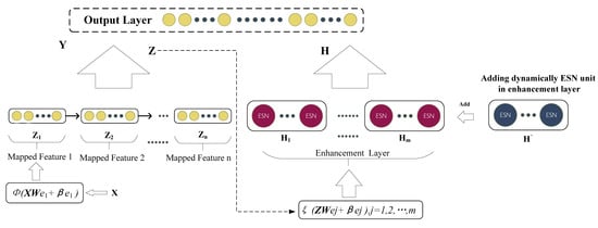
Figure 4.
The network structure of CMBESN.
The CMBESN model consists of the mapping, enhancement, and output layers. The ESN units are added to the enhancement layer with the incremental algorithm. The output of the mapping layer is shown in Formula (3). The output of the enhancement layer of the CMBESN is defined as:
, , and denote the output of the first ESN unit in the enhancement layer, the connection weight of the jth ESN unit to the mapping layer output, and the inner weights of the reserve pool in the jth ESN unit, respectively. Meanwhile, Z denotes the output of the mapping layer. The output and weight matrix of the CMBESN are calculated as follows.
The incremental algorithm is introduced in the CMBESN, which will be presented in Section 3.2. Then the combination matrix and the output weight matrix are changed as follows.
The pseudo-inverse matrix of the combination matrix is:
The updated output weight matrix is:
where are defined as follows:
The formulas above show that it does not need to restart the training data or recalculate when the incremental algorithm updates the network structure. and are updated with a simple matrix operation. The incremental algorithm can rapidly update the network model [30]. The training algorithm of the CMBESN is shown in Algorithm 1.
| Algorithm 1: The training algorithm of CMBESN |
| Input: Input data (after abnormal data processing and normalization, custom data step length), number of nodes in the mapping layer, RMSE threshold, spectral radius of ESN, leakage factor, and reserve pool size. |
| Output: Number of nodes in the enhancement layer, RMSE, training time. |
| Algorithm: |
| Step 1: Randomly initialize ; the initialized ESN unit includes the sparsity, the reservoir size, and the connection weight matrix. |
| Step 2: Record the output of mapping layer nodes . |
| Step 3: Record enhancement layer output . |
| Step 4: Calculate the combination matrix and the pseudo-inverse matrix of the combination matrix, and calculate the output weight matrix by Formulas (11) and (12). |
| Step 5: Calculate the current RMSE and compare it with the RMSE threshold. |
| Step 6: If the current prediction is greater than the RMSE threshold, the ESN unit is increased by the incremental algorithm. |
| Step 7: Initialize the newly added ESN cell by Step 1 and loop Step 4 to Step 6 to know that the RMSE of the prediction result is less than the RMSE threshold. |
| Step 8: Record training results. |
3.2. Optimization of Enhancement Layer Based on Unit Increment and Nonstationary Metrics
For the network proposed above, some measures should be taken to guarantee the performance of the CMBESN. A solution should determine the concrete structure and hyperparameter. Then the algorithms are studied in this section. Firstly, given the network structure, the number of ESN units is determined by an incremental algorithm. Secondly, in the view of the network hyperparameter, the regularization coefficient is adjusted based on the nonstationary metric of the time series. The two algorithms form the optimization of the enhancement layer.
3.2.1. Incremental Algorithm of Enhancement Units
The CMBESN and the ESN are introduced in the enhancement layer to fit the nonlinear trend of the data. The reserve pool is the essential component of the ESN, while its size is difficult to determine. Instead of the traditional empirical approach, an algorithm is designed to select the reservoir size automatically. The incremental algorithm can improve the fitting capability of the network by adjusting the number of ESN units in the enhancement layer. The flow of the incremental algorithm is shown in Algorithm 2.
| Algorithm 2: Incremental Algorithm |
| Input: Number of ESN, ESN parameter configuration, RMSE threshold. |
| Output: Output weight matrix . |
| Algorithm: |
| Step 1: Initialize mapping layer node parameters. |
| Step 2: Initialize the reinforced layer ESN cells, including reserve pool size, leakage factor, sparsity, etc. |
| Step 3: CEBESN network output before the incremental algorithm is used and is calculated. |
| Step 4: If is less than the RMSE threshold, incremental algorithm optimization is started. |
| Step 5: Calculate the current RMSE and compare it with the RMSE threshold. |
| Step 6: If the current prediction is greater than the RMSE threshold, the ESN unit is increased by the incremental algorithm. |
| Step 7: Update the combination matrix with by Formulas (14)–(18). |
| Step 8: Repeat step 5 to step 7 until is less than the RMSE threshold. Update at the same time. |
| Step 9: Record the last . |
The proposed algorithm above can help avoid the overfitting problem to a certain extent. It is conducted following the idea of early stopping. Early stopping is an iterative truncation method to prevent overfitting. The iteration stops before the model converges to the training data set. The accuracy of validation data is calculated at the end of each epoch. The accuracy is quantized with the RMES. The increment of the ESN units and training is stopped when the RMSE reaches the set condition.
3.2.2. Parameter Optimization Based on Nonstationary Metrics
Time series data are often nonstationary in complex systems [41]. The relationships in the nonstationary data are more complicated than that in the stationary time series [42]. The proposed network model is expected to be appropriate for the nonstationary time series. Then the parameters in CMBESN are optimized based on nonstationary time series data analysis.
In this paper, the parameters of CMBESN are optimized based on nonstationary metrics. Therefore, the test methods of the nonstationary time series are analyzed first. The classical test methods are Dickey-Fuller [43], augmented Dickey-Fuller (ADF) [44], correlation test [45], etc. The ADF test is a validation method to verify the stationarity of time series in classical econometric theory. The ADF test weakens the influence of the random disturbance term on the overall validation. It does not judge the stability of the time series with the existence of trailing and truncation such as the correlation test. The ADF criterion is the time series’ mean and variance. According to the Akaike information criterion (AIC), the degree of nonstationary is determined by judging the probability values (), test statistics, 1% critical value, 5% critical value, and 10% critical value.
The regularization coefficient in the CMBESN is vital for model training. The regularization coefficient is set as the parameter to optimize. This paper proposes an integrated metric consisting of the probability value from the ADF test and the model’s errors. The proposed nonstationary metric is as follows.
where and denote the ADF probability value of the predicted data and the ADF probability value of the actual data, respectively, represents the predicted value, means the true value, is the number of samples, is the set threshold coefficient, and denotes the nonstationary error indicator of the experiment. Combining the above indicators, can be calculated by the following formula:
where denotes the regularization coefficient of the CMBESN model at the prediction and represents the error of the actual data of the prediction series.
Formula (19) shows that the proposed metric can reflect the stability difference and the errors between predicted and actual data. Formula (20) is a function of stability difference. The smaller the , the smaller the prediction error. It can be seen from Formulas (22) and (23) that when the results are in the different intervals, the regularized scaling coefficients are adjusted to various degrees. Formula (21) is the termination condition of the optimization process. The optimization flow of the regularization coefficient is shown in Figure 5.
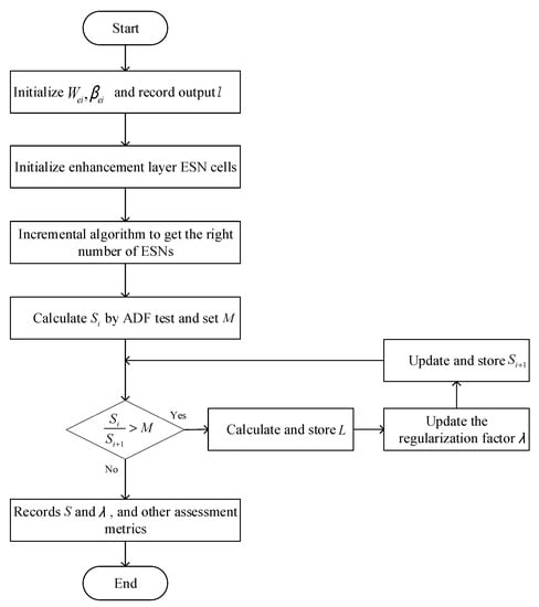
Figure 5.
Flow chart of optimization based on nonstationary error metrics.
As described above, the proposed CMBESN is optimized in the enhancement layer. Then it is abbreviated as CMBESN-OE, in which OE means optimizing the enhancement layer. The optimization includes the incremental algorithm of the ESN size and the parameter optimization based on the nonstationary metrics.
As a summary of the methods above, the training and test process of the CMBESN is shown in Figure 6. The related algorithms are shown in Table 2 and Table 3, and Figure 5.
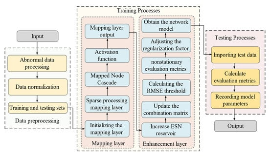
Figure 6.
The training and test process of the CMBESN-OE.
Table 2.
Configuration of model parameter for MSO dataset.
Table 2.
Configuration of model parameter for MSO dataset.
| Model | Number of Mapping Layer Nodes | Number of Enhancement Layer Nodes | Reservoir Size | Spectral Radius Rate | Leaking Rate | Sparseness |
|---|---|---|---|---|---|---|
| BLS | 1–50 | 1–40 | NA | NA | NA | NA |
| ESN | NA | NA | 300–800 | 0.95 | 0.1 | 0.05 |
| CMBLS | 1–50 | 1–40 | NA | NA | NA | NA |
| CMBESN | 1–50 | 1–40 | 300–800 | 0.95 | 0.1 | 0.05 |
Table 3.
Configuration of each model parameter in the Beijing Fangshan District air quality dataset.
Table 3.
Configuration of each model parameter in the Beijing Fangshan District air quality dataset.
| Model | Number of Mapping Layer Nodes | Number of Enhancement Layer Nodes | Reservoir Size | Spectral Radius Rate | Leaking Rate | Sparseness |
|---|---|---|---|---|---|---|
| BLS | 20–60 | 10–50 | NA | NA | NA | NA |
| ESN | NA | NA | 400–1000 | 0.95 | 0.1 | 0.05 |
| CMBLS | 20–60 | 10–50 | NA | NA | NA | NA |
| CMBESN | 20–60 | 10–50 | 400–1000 | 0.95 | 0.1 | 0.05 |
4. Experiment and Result
4.1. Dataset
4.1.1. Simulation Dataset
The data from the multiple superimposed oscillators (MSO) are the typical nonstationary time series, which are often used in the experiments of time series prediction. Kinds of frequency sine waves essentially form MSO data. In the real world, the superimposed phenomenon of multiple frequencies is widespread [46]. Then the data of MSO is set as the simulation data in the experiment. The complex degree increases rapidly when the number of superpositions rises. The MSO data can be expressed as follows.
where denotes the simulation sample, k represents the number of sinusoidal components, denotes the frequency of the component, and the frequency of each component in this paper is , Figure 7 shows the variation of MSO simulation data with eight components. To ensure the experiment’s reliability, the ratio of the training set to the test set is 4:1.
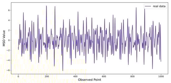
Figure 7.
MSO simulation data.
4.1.2. Air Quality Dataset
The air quality monitoring data in Fangshan District Beijing is a nonstationary time series dataset from the natural system. Air quality indexes include CO, NO2, O3, PM10, PM2.5, and SO2. The AQI is a comprehensive indicator reflecting the general air quality level. In the experiment, the AQI indicator is used as the output of prediction and the rest indicators as the input in this study. The dataset recorded 15,000 data. The monitoring started on 5 February 2017, and ended on 2 December 2018. The monitoring interval is 1 h. Figure 8 shows the general variation of AQI data in the dataset. The data were divided into a training set and a test set. The first 80% is the training set, and the remaining 20% is the test set.
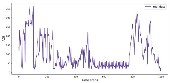
Figure 8.
AQI in air monitoring data of Fangshan District, Beijing.
It can be found from the figures above that the dataset used in the experiment is strongly nonstationary. There are different patterns in the data change, which helps avoid overfitting in the training since the model does not almost fall into a particular pattern. Meanwhile, the data size is large enough to cover different time series trends, which is also a measure to avoid overfitting.
4.2. Experimental Environment and Settings
The experiments are conducted on a platform with a 64-bit Windows system. Its memory is 16 GB, and the processor is AMD R7 4800H (2.9 GHz). The deep learning framework is based on Tensorflow 2.0 and Keras 2.4.3. The code is in Python 3.7 programming language.
To demonstrate the performance of the proposed CMBESN model, some typical methods in time series prediction are set as the contrast. The contrast models include the GRU, BLS, ESN, and CMBLS. The GRU is a classical model of RNN. The BLS, ESN, and CMBLS are the basic models for the proposed CMBESN. Then the four models are selected as the contrast.
The models above are trained for the two datasets to obtain relatively good results. The models are determined after the training. Table 2 and Table 3 show the parameters of models for the two datasets. The parameters include the number of nodes in the mapping layer, the number of nodes in the enhancement layer, the size of the reservoir in the ESN cell, the spectral radius of the reservoir, the leakage rate, and the sparsity of the reservoir.
For the prediction of time series, the evaluation metrics of model regression are usually chosen to verify the performance of the models. In this paper, the following metrics are taken, mean absolute deviation (MAE) [47], mean square root error (RMSE) [48], symmetric mean absolute percentage error (SMAPE) [49], and coefficient of determination R2 [50]. MAE, RMSE, and SMAPE reflect the deviation between the predicted and actual values. The smaller these three values are, the better the model performance is. R2 demonstrates the reasonableness of the final prediction model, and the closer R2 is to 1, the better the fit of the prediction model is. The formulas of the evaluation indexes are as follows:
where denotes the actual value of the sample, represents the predicted value of the sample, denotes the mean of the actual value, and denotes the number of samples.
4.3. Results
4.3.1. Results of MSO Dataset
The proposed CMBESN and the contrast models are applied in the prediction of the MSO data. The prediction results are shown in Figure 9. In the figure, the curves in different colors represent the models.
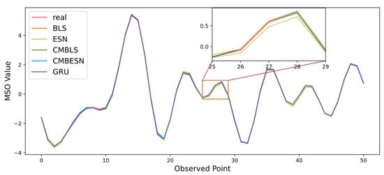
Figure 9.
Prediction results of each model on the MSO dataset.
To show the prediction results more obviously, the errors are drawn in Figure 10. In the figure, each bar indicates the absolute error value between the predicted and real values. It can be seen that the overall error value of CMBESN is small.
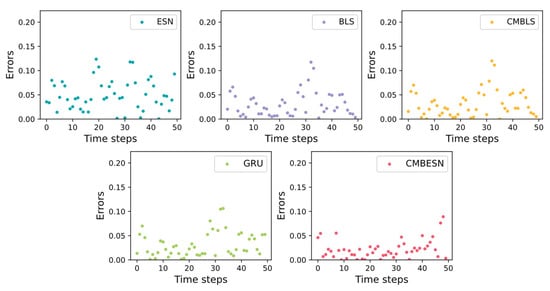
Figure 10.
Errors of each model on the MSO dataset.
To quantitatively analyze the performance of CMBESN, the evaluation metrics of ESN, BLS, CMBLS, GRU, and CMBESN are presented in the form of numerical values, as shown in Table 4.
Table 4.
Evaluation metrics for each model in the MSO dataset.
Figure 11 shows the decreased percentage of SMAPE, MAE, and RMSE and the increased percentage of R2 when the CMBESN is compared with other models.
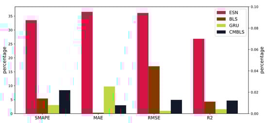
Figure 11.
Percentage change in evaluation metrics for CMBESN relative to each model on the MSO dataset.
4.3.2. Results of Air Quality Dataset
In this experiment of the air quality dataset, the predicted outputs are shown in Figure 12. It can be seen that the result of the CMBESN is closer to the actual values than other models in the general view.
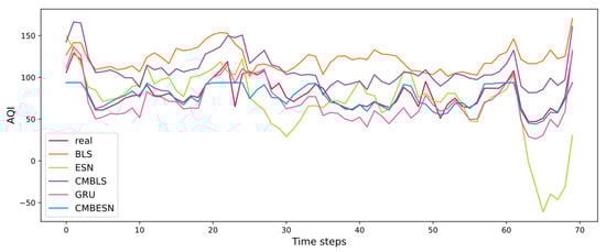
Figure 12.
Prediction results of each model in the air quality data set of Fangshan District, Beijing.
For further comparison of the results, the outputs are plotted with the boxplots in Figure 13. The middle horizontal line and the start point in each box represent the median and mean of the data. The size of the box indicates the distribution of the data. As seen in Figure 13, the mean and median of CMBESN are closest to the actual data.
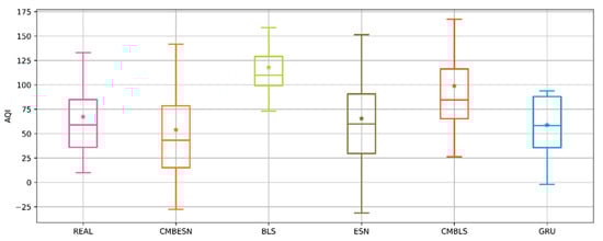
Figure 13.
Boxplot of the prediction results of each model for the air quality dataset.
For a clear comparison, the models’ errors are shown in Figure 14. It can be seen that the error variation range of CMBESN is much smaller than that of CMBLS, ESN, and GRU, which means that CMBESN has a higher prediction accuracy and fits the real curve most closely.
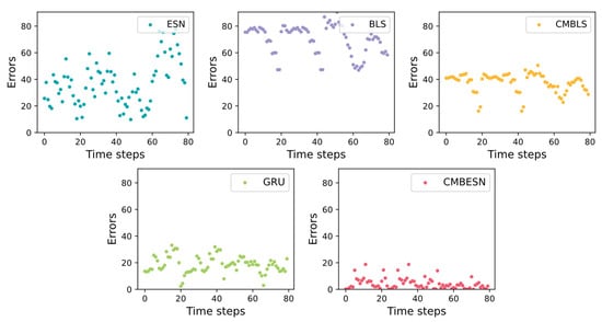
Figure 14.
Errors of each model on air quality dataset.
The evaluation metrics are shown in Table 5, which contains the training time, RMSE, SMAPE, MAE, and R2 for each model.
Table 5.
Evaluation metrics for each model on the air quality dataset.
Figure 15 shows the decreased percentage of SMAPE, MAE, RMSE, and the increased ratio of R2 when the CMBESN is compared with other models on the air quality dataset.
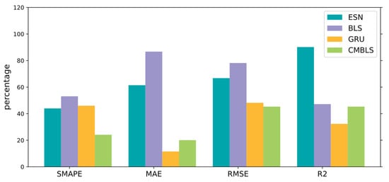
Figure 15.
Percentage change in evaluation metrics for CMBESN relative to each model on the air quality dataset.
As seen in Table 5, the BLS model performs the worst performance. CMBLS improves performance over BLS. CMBESN improves accuracy over other networks. Meanwhile, Figure 15 shows the decreased percentage in RMSE, SMAPE, and MAE and the increased percentage in R2 for CMBESN, which means the CMBESN has a better performance. It can also be seen that the CMBESN model has the slightest prediction error. The training time is also shorter than GRU.
The proposed CMBESN Is tested in the experiment by comparing some related models. It can be found from the results that the prediction accuracy of the CMBESN has been improved. However, the training time has risen at the same time. Then the model should be optimized, and the experiments are conducted in Section 4.4.
4.4. Optimization Experiments
4.4.1. Optimization Results of MSO Dataset
The proposed optimization method is tested based on the CMBESN model. Then a CMBESN model is selected with 34 nodes in the mapping layer, 24 nodes in the enhancement layer, and a reservoir pool size of 550 neural nodes. The optimized CMBESN is abbreviated as CMBESN-OE, mentioned in Section 3.2.2.
The variation of RMSE and regularization coefficient of the CMBESN-OE model during the optimization is shown in Figure 16. It is set that in Formula (22). It can be seen that the first eight adjustments have a noticeable effect on the optimization process. The RMSE shows a definite downward trend. When the regularization coefficient is adjusted, the RMSE tends to be stable, which means the optimization saturation.
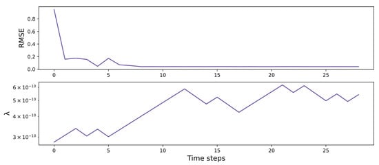
Figure 16.
RMSE and λ variation curves of CMBESN-OE model on MSO dataset.
The prediction curves of the CMBESN and CMBESN-OE models are plotted in Figure 17 when the RMSE tends to be stable in the optimization. For a clear comparison, the errors of the two models are shown in Figure 18.
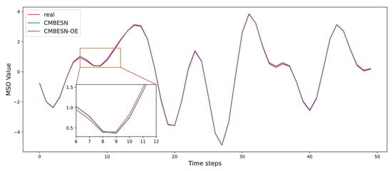
Figure 17.
Prediction curves of CMBESN and CMBESN-OE models on MSO dataset.
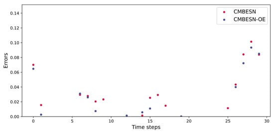
Figure 18.
Errors of CMBESN and CMBESN-OE models on MSO dataset.
The evaluation metrics of the prediction results are calculated, as shown in Table 6.
Table 6.
Evaluation metrics of CMBESN and CMBESN-OE models on MSO dataset.
As seen in Table 6, the CMBESN-OE with the optimization performs better than the CMBESN model. It proves that the optimization algorithm can improve the CMBESN model to a certain extent on the MSO dataset.
4.4.2. Optimization Results of Air Quality Dataset
Similar to the optimization experiment of the MSO dataset, the air quality dataset is tested. A CMBESN model is selected with 36 nodes in the mapping layer, 28 nodes in the enhancement layer, and a reservoir pool size of 600. The CMBESN-OE model is obtained by optimizing the CMBESN with the optimization algorithm mentioned in Section 3.2.2 and setting in the subset.
The CMBESN-OE is used to optimize the regularization coefficient in Formula (19). Then the trend of RMSE and is plotted in Figure 19, which shows that the RMSE has reached a smaller value by the 34th adjustment and shows a decreasing trend in general.
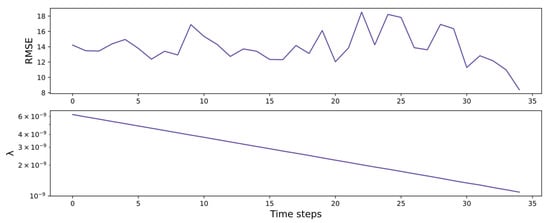
Figure 19.
RMSE and λ variation curves of CMBESN-OE model on air quality dataset.
The CMBESN-OE model reaches a better state after 34 times of optimization. The results are shown in Figure 20. It indicates that the CMBESN-OE generally fits the actual data curve better.
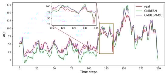
Figure 20.
Prediction curves of CMBESN and CMBESN-OE models on air quality dataset.
The evaluation metrics of the two models are shown in Table 7. It indicates that CMBESN-OE performs better than CMBESN in all evaluation metrics.
Table 7.
Evaluation metrics of CMBESN and CMBESN-OE models on air quality dataset.
5. Discussion and Conclusions
The CMBESN model proposed in this paper is validated on the simulation dataset of MSO and Beijing air quality dataset. The classical deep learning network and the broad learning system are compared. The CMBESN-OE model based on the optimization method is also validated on both datasets. The model testing strategy uses a similar approach to K-fold cross-validation, and the results shown in this paper are the better-performing prediction data after the selection.
From the result curves in Figure 8 and Figure 10, it can be seen that the CMBESN model fits the actual data curve more closely than the BLS, ESN, CMBLS, and GRU models, especially at the peaks. The errors between the predicted and actual values are shown in Figure 10 and Figure 14. The CMBESN model performs better, especially in the air quality dataset. The models can be evaluated quantificationally using the metrics in Table 6 and Table 7. For the MSO dataset, the RMSE of CMBESN decreases by 36.1%, 1.7%, 0.98%, and 4.9% relative to ESN, BLS, GRU, and CMBLS, respectively. The R2 improves by 0.01% and 0.07% relative to BLS and CMBLS. For the air quality dataset, the RMSE of CMBESN decreases by 66.8%, 78.1%, 48.2%, and 45.3% relative to ESN, BLS, GRU, and CMBLS, respectively. However, given the time cost, CMBESN takes more time to train the model. The tradeoff between prediction accuracy and the time cost can be studied in the future.
The CMBESN-OE model derives from the CMBESN based on the optimization algorithms. The concrete structure parameter and hyperparameter of the CMBESN are determined with the algorithms in Section 3.2. The related experiments are shown in Section 4.4. The results in Figure 18 and Figure 20 show that the errors of the CMBESN-OE model are smaller than the CMBESN. Figure 16 and Figure 19 show the RMSE and the regularization coefficient changing along the optimization process. The RMSEs decline obviously with the variation of the optimized parameter. Similar conclusions can be found in Table 6 and Table 7. It proves that the optimization proposed in this paper is efficient. The proposed algorithms can improve prediction accuracy by adjusting the structure and training parameters.
In this paper, a new network is designed and studied for time series prediction. The broad echo state network is improved in the mapping and enhancement layers. It is proved with the experiment that the proposed network can take advantage of the BLS and ESN. Meanwhile, the optimization method is also studied to improve the prediction ability. In the future, the theoretical foundation should be studied to explain the further reason for the combination of the networks. Besides, the combination has taken more time, which can be found in the experiments. Then, the proposed network should be improved from the training time. An ideal network should be explored based on the proposed method in this paper to balance the prediction accuracy and the computational resources.
Author Contributions
Conceptualization, W.-J.L. and Y.-T.B.; methodology, W.-J.L. and Y.-T.B.; writing—original draft preparation, W.-J.L., Y.-T.B. and X.-B.J.; writing—review and editing, W.-J.L. and Y.-T.B.; funding acquisition, Y.-T.B., X.-B.J., J.-L.K. and T.-L.S. All authors have read and agreed to the published version of the manuscript.
Funding
This work was partly supported by the National Key Research and Development Program of China No. 2020YFC1606801, National Natural Science Foundation of China Nos. 62173007, 61903009, 62006008.
Institutional Review Board Statement
Not applicable.
Informed Consent Statement
Not applicable.
Data Availability Statement
The data presented in this study are available on request from the corresponding author.
Conflicts of Interest
The authors declare no conflict of interest.
References
- Harris, E.; Coleman, R. The social life of time and methods: Studying London’s temporal architectures. Time Soc. 2020, 29, 604–631. [Google Scholar] [CrossRef]
- Xu, L.; Li, Q.; Yu, J.; Wang, L.; Xie, J.; Shi, S. Spatio-temporal predictions of SST time series in China’s offshore waters using a regional convolution long short-term memory (RC-LSTM) network. Int. J. Remote Sens. 2020, 41, 3368–3389. [Google Scholar] [CrossRef]
- Shi, Z.; Bai, Y.; Jin, X.; Wang, X.; Su, T.; Kong, J. Parallel deep prediction with covariance intersection fusion on nonstationary time series. Knowl.-Based Syst. 2021, 211, 106523. [Google Scholar] [CrossRef]
- Taylor, S.J. Modelling Financial Time Series; World Scientific: Singapore, 2008. [Google Scholar]
- Kong, J.; Wang, H.; Wang, X.; Jin, X.; Fang, X.; Lin, S. Multi-stream hybrid architecture based on cross-level fusion strategy for fine-grained crop species recognition in precision agriculture. Comput. Electron. Agric. 2021, 185, 106134. [Google Scholar] [CrossRef]
- Kong, J.; Wang, H.; Yang, C.; Jin, X.; Zuo, M.; Zhang, X. Fine-grained pests & diseases recognition via Spatial Feature-enhanced attention architecture with high-order pooling representation for Precision Agriculture Practice. Agriculture 2022, 2022, 1592804. [Google Scholar]
- Jin, X.B.; Zheng, W.Z.; Kong, J.L.; Wang, X.Y.; Bai, Y.T.; Su, T.L.; Lin, S. Deep-learning forecasting method for electric power load via attention-based encoder-decoder with Bayesian optimization. Energies 2021, 14, 1596. [Google Scholar] [CrossRef]
- Jin, X.-B.; Zheng, W.-Z.; Kong, J.-L.; Wang, X.-Y.; Zuo, M.; Zhang, Q.-C.; Lin, S. Deep-learning temporal predictor via bidirectional self-attentive encoder–decoder framework for IOT-based environmental sensing in intelligent greenhouse. Agriculture 2021, 11, 802. [Google Scholar] [CrossRef]
- Jin, X.B.; Gong, W.T.; Kong, J.L.; Bai, Y.T.; Su, T.L. A variational Bayesian deep network with data self-screening layer for massive time-series data forecasting. Entropy 2022, 24, 355. [Google Scholar] [CrossRef]
- Kong, J.; Yang, C.; Wang, J.; Wang, X.; Zuo, M.; Jin, X.; Lin, S. Deep-stacking network approach by multisource data mining for hazardous risk identification in iot-based intelligent food management systems. Comput. Intell. Neurosci. 2021, 2021, 1194565. [Google Scholar] [CrossRef]
- Jin, Z.C.; Zhou, X.H.; He, J. Statistical methods for dealing with publication bias in meta-analysis. Stat. Med. 2015, 34, 343–360. [Google Scholar] [CrossRef]
- Austin, P.C. Comparing paired vs. non-paired statistical methods of analyses when making inferences about absolute risk reductions in propensity-score matched samples. Stat. Med. 2011, 30, 1292–1301. [Google Scholar] [CrossRef] [PubMed] [Green Version]
- Yariyan, P.; Janizadeh, S.; Van Phong, T.; Nguyen, H.D.; Costache, R.; Van Le, H.; Pham, B.T.; Pradhan, B.; Tiefenbacher, J.P. Improvement of best first decision trees using bagging and dagging ensembles for flood probability mapping. Water Resour. Manag. 2020, 34, 3037–3053. [Google Scholar] [CrossRef]
- Daneshfaraz, R.; Bagherzadeh, M.; Esmaeeli, R.; Norouzi, R.; Abraham, J. Study of the performance of support vector machine for predicting vertical drop hydraulic parameters in the presence of dual horizontal screens. Water Supply 2021, 21, 217–231. [Google Scholar] [CrossRef]
- Tang, W.H.; Röllin, A. Model identification for ARMA time series through convolutional neural networks. Decis. Support Syst. 2021, 146, 113544. [Google Scholar] [CrossRef]
- Abueidda, D.W.; Koric, S.; Sobh, N.A.; Sehitoglu, H. Deep learning for plasticity and thermo-viscoplasticity. Int. J. Plast. 2021, 136, 102852. [Google Scholar] [CrossRef]
- Jin, X.-B.; Gong, W.-T.; Kong, J.-L.; Bai, Y.-T.; Su, T.-L. PFVAE: A planar flow-based variational auto-encoder prediction model for time series data. Mathematics 2022, 10, 610. [Google Scholar] [CrossRef]
- Cho, K.; Kim, Y. Improving streamflow prediction in the WRF-Hydro model with LSTM networks. J. Hydrol. 2022, 605, 127297. [Google Scholar] [CrossRef]
- Chen CL, P.; Liu, Z.; Feng, S. Universal approximation capability of broad learning system and its structural variations. IEEE Trans. Neural Netw. Learn. Syst. 2018, 30, 1191–1204. [Google Scholar] [CrossRef]
- Shi, Z.; Bai, Y.; Jin, X.; Wang, X.; Su, T.; Kong, J. Deep Prediction Model Based on Dual Decomposition with Entropy and Frequency Statistics for Nonstationary Time Series. Entropy 2022, 24, 360. [Google Scholar] [CrossRef]
- Mohammadpour, M.; Soltani, A.R. Forward Moving Average Representation in Multivariate MA (1) Processes. Commun. Stat. Theory Methods 2010, 39, 729–737. [Google Scholar] [CrossRef]
- Singh, S.N.; Mohapatra, A. Repeated wavelet transform based ARIMA model for very short-term wind speed prediction. Renew. Energy 2019, 136, 758–768. [Google Scholar]
- Akbar, S.B.; Govindarajan, V.; Thanupillai, K. Prediction Bitcoin price using time opinion mining and bi-directional GRU. J. Intell. Fuzzy Syst. 2022, 42, 1–9. [Google Scholar]
- Ma, M.; Liu, C.; Wei, R.; Liang, B.; Dai, J. Predicting machine’s performance record using the stacked long short-term memory (LSTM) neural networks. J. Appl. Clin. Med. Phys. 2022, 23, e13558. [Google Scholar] [CrossRef] [PubMed]
- Gallicchio, C.; Micheli, A.; Silvestri, L. Local lyapunov exponents of deep echo state networks. Neurocomputing 2018, 298, 34–45. [Google Scholar] [CrossRef]
- Kong, J.; Yang, C.; Xiao, Y.; Lin, S.; Ma, K.; Zhu, Q. A Graph-Related High-Order Neural Network Architecture via Feature Aggregation Enhancement for Identification Application of Diseases and Pests. Comput. Intell. Neuro-Sci. 2022, 2022, 4391491. [Google Scholar] [CrossRef]
- Jin, X.-B.; Yu, X.-H.; Su, T.-L.; Yang, D.-N.; Bai, Y.-T.; Kong, J.-L.; Wang, L. Distributed deep fusion predictor for a multi-sensor system based on causality entropy. Entropy 2021, 23, 219. [Google Scholar] [CrossRef]
- Sherstinsky, A. Fundamentals of recurrent neural network (RNN) and long short-term memory (LSTM) network. Phys. D Nonlinear Phenom. 2020, 404, 132306. [Google Scholar] [CrossRef] [Green Version]
- Bai, Y.; Zhao, Z.; Wang, X.; Jin, X.; Zhou, B. Continuous Positioning with Recurrent Auto-Regressive Neural Network for Unmanned Surface Vehicles in GPS Outages. Neural Process. Lett. 2022, 54, 1413–1434. [Google Scholar] [CrossRef]
- Chen, C.L.P.; Liu, Z. Broad learning system: An effective and efficient incremental learning system without the need for deep architecture. IEEE Trans. Neural Netw. Learn. Syst. 2017, 29, 10–24. [Google Scholar] [CrossRef]
- Jin, X.; Zhang, J.; Kong, J.; Su, T.; Bai, Y. A reversible automatic selection normalization (RASN) deep network for predicting in the smart agriculture system. Agronomy 2022, 12, 591. [Google Scholar] [CrossRef]
- Li, H.; Sun, W.; Zhou, Z.; Li, C.; Zhang, S. Human Sitting-Posture Recognition Based on the Cascade of Feature Mapping Nodes Broad Learning System. J. Nantong Univ. (Nat. Sci. Ed.) 2020, 19, 28–33. [Google Scholar]
- Feng, S.; Chen, C.L.P.; Xu, L.; Liu, Z. On the Accuracy–Complexity Tradeoff of Fuzzy Broad Learning System. IEEE Trans. Fuzzy Syst. 2020, 29, 2963–2974. [Google Scholar] [CrossRef]
- Liu, W.; Bai, Y.; Jin, X.; Wang, X.; Su, T.; Kong, J. Broad Echo State Network with Reservoir Pruning for Nonstationary Time Series Prediction. Comput. Intell. Neurosci. 2022, 2022, 3672905. [Google Scholar] [CrossRef] [PubMed]
- Li, D.; Han, M.; Wang, J. Chaotic time series prediction based on a novel robust echo state network. IEEE Trans. Neural Netw. Learn. Syst. 2012, 23, 787–799. [Google Scholar] [CrossRef] [PubMed]
- Hoerl, A.E.; Kennard, R.W. Ridge regression: Biased estimation for nonorthogonal problems. Technometrics 1970, 12, 55–67. [Google Scholar] [CrossRef]
- Jaeger, H. Adaptive nonlinear system identification with echo state networks. Adv. Neural Inf. Proces. Syst. 2002, 15, 609–616. [Google Scholar]
- Li, D.; Liu, F.; Qiao, J. Research on hierarchical modular ESN and its application. In Proceedings of the 2015 34th Chinese Control Conference (CCC), Hangzhou, China, 28–30 July 2015; pp. 2129–2133. [Google Scholar]
- Jordan, S.; Philips, A.Q. Cointegration testing and dynamic simulations of autoregressive distributed lag models. Stata J. 2018, 18, 902–923. [Google Scholar] [CrossRef] [Green Version]
- Erdem, E.; Shi, J. ARMA based approaches for prediction the tuple of wind speed and direction. Appl. Energy 2011, 88, 1405–1414. [Google Scholar] [CrossRef]
- Xie, C.; Bijral, A.; Ferres, J.L. Nonstop: A nonstationary online prediction method for time series. IEEE Signal Proces. Lett. 2018, 25, 1545–1549. [Google Scholar] [CrossRef] [Green Version]
- Osogami, T. Second order techniques for learning time series with structural breaks. In Proceedings of the AAAI Conference on Artificial Intelligence, Vancouver, BC, Canada, 2–9 February 2021; Volume 35, pp. 9259–9267. [Google Scholar]
- Dolado, J.J.; Gonzalo, J.; Mayoral, L. A fractional Dickey–Fuller test for unit roots. Econometrica 2002, 70, 1963–2006. [Google Scholar] [CrossRef] [Green Version]
- Bisaglia, L.; Procidano, I. On the power of the augmented Dickey–Fuller test against fractional alternatives using bootstrap. Econ. Lett. 2002, 77, 343–347. [Google Scholar] [CrossRef]
- Xie, Y.; Liu, S.; Fang, H.; Wang, J. Global autocorrelation test based on the Monte Carlo method and impacts of eliminating nonstationary components on the global autocorrelation test. Stoch. Environ. Res. Risk Assess. 2020, 34, 1645–1658. [Google Scholar] [CrossRef]
- Thornhill, N.F.; Huang, B.; Zhang, H. Detection of multiple oscillations in control loops. J. Process Control 2003, 13, 91–100. [Google Scholar] [CrossRef] [Green Version]
- Ni, T.; Wang, L.; Zhang, P.; Wang, B.; Li, W. Daily tourist flow forecasting using SPCA and CNN-LSTM neural network. Concurr. Comput. Pract. Exp. 2021, 33, e5980. [Google Scholar] [CrossRef]
- Liao, Y.; Li, H. Deep echo state network with reservoirs of multiple activation functions for time-series forecasting. Sādhanā 2019, 44, 1–12. [Google Scholar] [CrossRef] [Green Version]
- Chen, C.; Twycross, J.; Garibaldi, J.M. A new accuracy measure based on bounded relative error for time series forecasting. PLoS ONE 2017, 12, e0174202. [Google Scholar] [CrossRef] [Green Version]
- Kim, S.; Alizamir, M.; Zounemat-Kermani, M.; Kisi, O.; Singh, V.P. Assessing the biochemical oxygen demand using neural networks and ensemble tree approaches in South Korea. J. Environ. Manag. 2020, 270, 110834. [Google Scholar] [CrossRef]
Publisher’s Note: MDPI stays neutral with regard to jurisdictional claims in published maps and institutional affiliations. |
© 2022 by the authors. Licensee MDPI, Basel, Switzerland. This article is an open access article distributed under the terms and conditions of the Creative Commons Attribution (CC BY) license (https://creativecommons.org/licenses/by/4.0/).