Extraction of Catastrophe Boundary and Evolution of Expressway Traffic Flow State

Abstract

As the main road type in an urban traffic system, the increasingly severe congestion of the expressway restricts social and economic development. It is essential to explore the evolution law of congestion and dissipation to ensure the efficient operation of the expressway. In order to accurately grasp the evolution law of the expressway traffic flow state, this paper selects the expressway weaving section, which is a traffic flow frequency-changing area, to study the traffic operation state, change process, and evolution law, and determine the traffic state discrimination standard. The simulation analysis was carried out using the traffic simulation platform, Vissim software. The simulation results showed an apparent catastrophe phenomenon in the mutual transformation between free and congestion flow. The spectral clustering analysis algorithm was used to accurately extract the boundary of traffic state mutation, combined with the cusp catastrophe theory, to study and analyze the traffic flow state at different times and positions, thus completely displaying the evolution characteristics of traffic flow state. The research results provide an essential theoretical basis for formulating control measures of expressway traffic flow and strategies for traffic congestion dissipation.

1. Introduction

As the hub of urban transportation, the urban expressway plays an essential role in increasing traffic carrying capacity, improving road service level, and strengthening vehicle operation efficiency in urban transportation systems. With the development of the urban expressway system and the encryption of the road network, the intersection of the urban expressway and ground roads increases, and many complex traffic bottlenecks inevitably appear in the intersection areas and weaving sections, causing traffic congestion. The low efficiency of urban expressways has been criticized for a long time; hence, it is urgent to control and solve the congestion problem. Research on urban expressway traffic congestion formation and the evolution law of dissipation, along with probes into its evolution mechanism from the angle of time and space, can help target the management of expressway traffic to improve the efficiency of urban road network traffic.

Research on the evolution law of traffic flow states has a long history. The traditional research method is to establish the fundamental diagram model [1] or LWR (Lighthill–Whitham–Richards) model [2,3] according to the fundamental relationship among the three parameters of traffic volume, speed, and density, and to elaborate on the traffic flow state by studying the functional relationship. Hao [4] abstracted vehicles into interacting molecules, analyzed the influence of vehicle movement trends on traffic flow using molecular dynamics, and explored its evolution law, in combination with the basic theory of the cellular automata model. Zhang [5] analyzed and discussed the correlation relationship between parameters according to the variation tendency of system traffic volume in the phase transformation process and obtained the corresponding parameter correlation function, which can better describe the correlation evolution law between traffic flow parameters. On the basis of the LWR model, Wang [6] proposed the concept of density-dependent relaxation time and expounded on the evolution law of traffic flow state by studying the density distribution and speed boundary perturbation. Hattam [7] simplified the optimal velocity model using the perturbed modified Korteweg–de Vries (mKdV) equation within the unstable regime; steady traveling wave solutions to this equation were then derived using a multiscale perturbation technique, thereby describing the evolution process of congestion.

Later, with the advancement of data acquisition technology, many scholars captured the evolution mechanism of traffic flow state by processing a large amount of traffic flow data. Younes [8] used Internet of vehicles technology to analyze traffic volume, speed, and travel time, and a congestion detection algorithm was proposed to explore the evolution process of congestion with travel time. Fei [9] proposed a practical approach for predicting the congestion boundary due to traffic incidents. Each road type’s essential congestion propagation speed was calculated using remote traffic microwave sensors and floating vehicle data systems to capture the congestion propagation characteristics in the existing road network. Li [10] studied the influence of variable speed limits on the evolution of traffic flow by combining the current emerging complex network theory with the improved traffic flow simulation model. Hu [11] took the standard section of the expressway as an example, simulated the real-time operating state of traffic flow with the help of Vissim traffic simulation software, analyzed its evolution process, and explored the discrimination standards and methods of different traffic flow states. Ghadami [12] exploited the phenomenon of critical slowing down in dynamic systems near bifurcation, i.e., traffic congestion, to predict the evolution law of traffic congestion after bifurcation by using a few traffic measurements before the tipping point occurs. Shao [13] studied the evolution law of traffic flow state by determining the critical change nodes of urban road traffic flow state using the profile of the equilibrium model of cusp catastrophe theory.

In recent years, machine learning algorithms have gradually emerged. When applied to transportation, they can significantly improve the accuracy and reliability of traffic flow data processing. Chaurasia [14] combined data mining historical trajectory data to detect and predict traffic congestion and used the track clustering algorithm to study the evolution law of road bottleneck formation and proposed a solution to reduce congestion. Lin [15] used a k-means clustering algorithm to put forward a quantitative method that can effectively identify traffic state offline to analyze its evolution law. Liu [16] proposed a neural network to calculate vehicles’ relative position and speed on the expressway to monitor the traffic volume and analyze the traffic flow state. Gao [17] studied a vehicle wireless positioning fusion algorithm suitable for the actual vehicle–road collaborative environment, which can help identify real-time traffic congestion status and other practical scenarios all day.

As reviewed in this section, it can be seen that studies on the evolution law of traffic flow state are relatively mature. However, most of them were based on the continuous traffic flow model using a two-dimensional surface, which struggles to explain the discontinuous catastrophe phenomenon in complex three-dimensional traffic data. Moreover, in the limited studies on the catastrophe phenomenon of traffic flow state, the length of catastrophe interval was chiefly set artificially. Then, the interval corresponding to the minor data within this length was found by traversing the sample set as the range of the catastrophe interval, easily leading to insufficient accuracy and reliability.

This paper introduces the cusp catastrophe theory based on the traffic flow theory. It applies a new spectral clustering algorithm to improve the catastrophe boundary extraction method to establish a calculation model and criteria that are more in line with the actual traffic flow state of the expressway. This method can achieve the goal of distinguishing the traffic flow state of the expressway and accurately describing its evolution law to accurately evaluate and predict the traffic flow state of the road network, analyze and mine the evolution mechanism of traffic congestion, and make a reasonable judgment on the development of traffic state.

The remainder of the paper is organized as follows: Section 2 introduces the cusp catastrophe theory and analyzes the catastrophe characteristics of the traffic flow state on the basis of simulation data. Section 3 uses the spectral clustering analysis algorithm to accurately extract the boundary of catastrophe interval of traffic flow state. Then, a sensitivity analysis of the critical factors affecting the velocity catastrophe boundary is carried out. Furthermore, the accuracy of the method is verified using an example. In Section 4, on the basis of the cusp catastrophe theory, we conduct a comprehensive and detailed analysis of the evolution law of urban expressway traffic flow state from the aspects of traffic volume, speed, occupancy rate, and different spatial and temporal distribution. Lastly, we outline the conclusions in Section 5.

2. Analysis of Catastrophe Characteristics of Traffic Flow

2.1. Cusp Catastrophe Theory

Cusp catastrophe theory explores the intrinsic mechanism of a catastrophe from one steady state to another steady state in a system by establishing a catastrophe model [18]. According to the catastrophe theory, the system can be divided into two modes: steady-state continuity and unsteady discontinuity. The state change of the system is realized through the transformation of the two modes. During the system’s evolution, when one or more factors change continuously, there may be a noncontinuous catastrophe in one of the factors, resulting in a change in the overall situation of the system. This change in state mode can be analyzed by studying the potential function of the system. In the catastrophe theory model, there are control variables and state variables. With the continuous changes of the control variables, the state variables change suddenly. By constructing the state space and control space, the boundary points of the system’s equilibrium state can be obtained. Catastrophe theory analyzes the catastrophe characteristics of the system according to the mutual transformation between the research boundary points.

When catastrophe theory is applied to traffic flow systems [19,20], the traffic volume and occupancy rate are the control variables, and speed is the state variable in traffic flow evolution. Catastrophe theory describes the phenomenon between two steady states of free and congested flow. In addition, to accurately define the catastrophe interval in the model, the concept of synchronized flow is introduced in this paper [21]. With the continuous increase in traffic volume, the following distance of vehicles gradually decreases during operation, the vehicles drive evenly on the road, and the speed gradually reaches synchronization, representing a synchronized flow state. At this time, there is a strong interaction between vehicles, and a slight disturbance may change their running state.

The fundamental theoretical model of cusp catastrophe is expressed as follows [22]:

$$F(x)=a{x}^4+by{x}^2+czx,$$

(1)

where x is the state variable, and y is the control variable.

In order to conform to the traffic flow theory, variables are converted into traffic flow parameters.

$$F(v)=a{v}^4+bq{v}^2+cov.$$

(2)

The equilibrium surface equation is obtained by derivation.

$$4a{v}^3+2bqv+co=0.$$

(3)

The singularity set equation is obtained by further derivation.

$$12a{v}^2+2bq=0$$

(4)

Equations (3) and (4) can be combined to eliminate v, thereby yielding the bifurcation set.

$$8b{q}^3+27a{c}^2{o}^2=0,$$

(5)

where $v$ is the state variable of speed (km·h⁻¹), $q$ is the control variable of traffic volume ($pcu$), $o$ is the control variable of time occupancy ($\%$), and $a,b,c$ are parameters.

In order to satisfy the cusp catastrophe theory, fundamental data transformation is required when traffic flow parameters are applied to the catastrophe theory.

(1)

Coordinate translation:

$$\{\begin{array}{l}{v}_1=v_0-v_{q_m}\\ q_1=q_0-q_m\\ o_1=o_0-o_{q_m}\end{array},$$

(6)

where $v_{q_m}$ is the optimal speed at maximum traffic volume (km·h⁻¹), $q_m$ is the maximum traffic ($pcu$), and $o_{q_m}$ is the time occupancy at maximum traffic volume ($\%$).

(2)

Coordinate rotation:

$$\{\begin{array}{l}{v}_2=v_1\\ q_2=q_1\cos \theta -m{o}_1\sin \theta \\ o_2=q_1\sin \theta +m{o}_1\cos \theta \end{array},$$

(7)

where m is the graphic factor, whose value is $q_m/o_{q_m}$, and $\theta$ is the rotation angle (°).

Equilibrium surface equation after transformation:

$$v_2^3+a{q}_2{v}_2+b{o}_2=0.$$

(8)

2.2. Analysis of Catastrophe Characteristics of Traffic Flow

The expressway weaving section is an area where vehicle lane-changing occurs frequently. Many instances of vehicle weaving result in a frequently congested section; thus, it can be considered a critical research object. Because field investigations have a huge workload and it is challenging to extract representative data for targeted problems, a combination of field investigation and simulation was used for data collection.

The weaving section of Hang’an Expressway at Anshan No. 2 Road in Qingdao was selected as the investigation site. Through video detection and the GPS (Global Positioning System) floating car method [23,24], the length, number of lanes, traffic volume, and other parameters of the weaving section could be effectively investigated. The investigation period was from 22 to 26 November 2021, taking this real scenario as the research object. Using the traffic simulation platform Vissim, the field investigation results were used as input parameters to build a scenario for data simulation. The specific scheme of traffic simulation was as follows:

(1)

Simulation scenario: According to the survey results, the mainline of the expressway was a two-way six-lane straight section, the length of the weaving section was 210 m, the lane width was 3.75 m, and the simulation interval was 1000 m.

(2)

Traffic volume: According to the actual investigation, it was found that the traffic volume in this weaving section was 1200–3700 pcu/h in 1 day; thus, the calibration simulation traffic volume was 1000–4000 pcu/h, the step length was 500 pcu/h, and the simulation time of each interval step length was 3600 s.

(3)

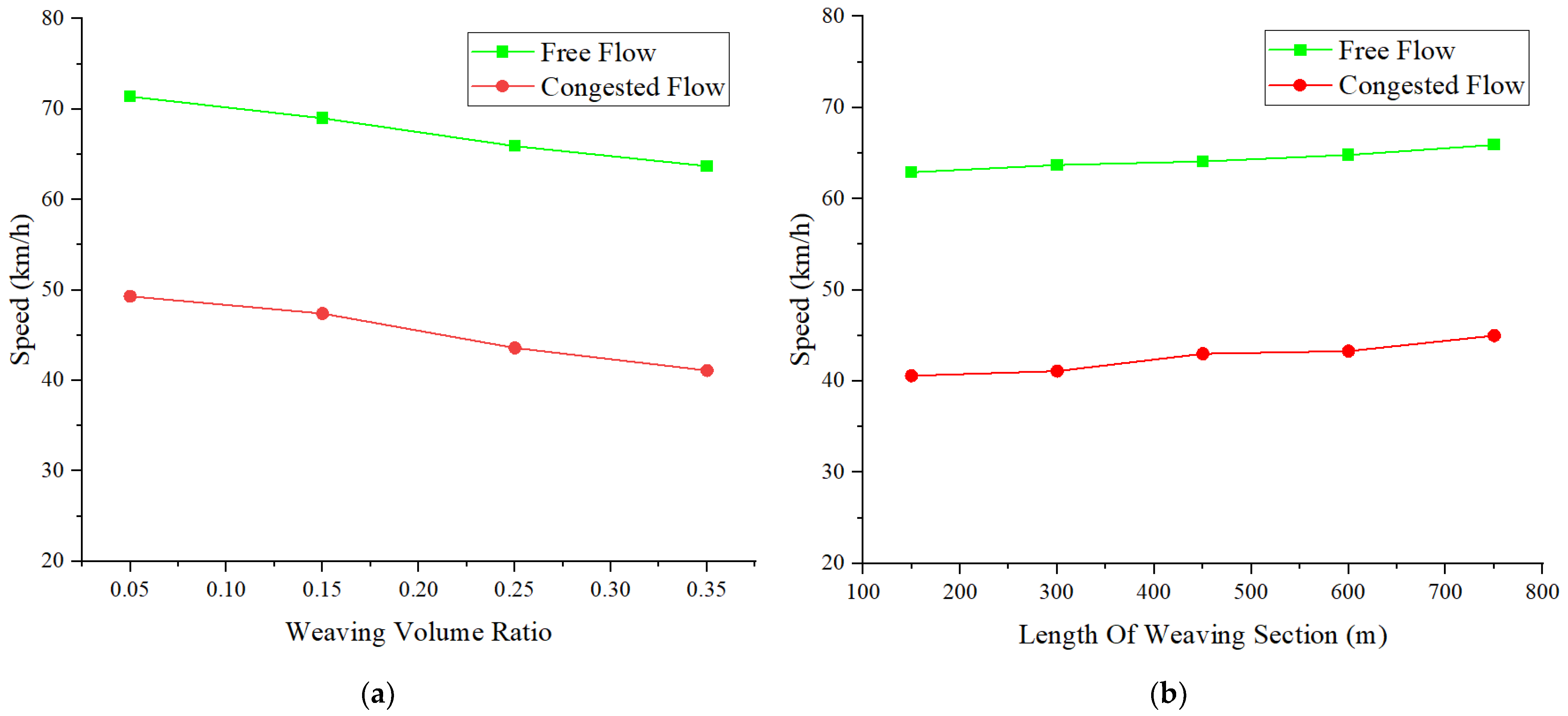
Weaving volume ratio: In order to study the congestion characteristics of the weaving section, according to the “Highway Capacity Manual”, the maximum weaving volume ratio for a weaving section with four lanes was selected as 0.35.

(4)

Traffic composition: According to the actual survey results, there were few large vehicles on expressways in the city, with small vehicles accounting for 0.98 and large vehicles accounting for 0.02.

(5)

Expected speed: According to the actual investigation results, the expected speed of the mainline of the expressway was set as 80 km/h, and the expected speed of the ramp was set as 40 km/h. The vehicle speed conformed to a Weibull distribution.

(6)

Driver behavior: The action point model of the Vissim simulation platform was used to describe the drivers’ behavior.

(7)

Data detection: According to the “Highway Capacity Manual”, the weaving section ranged from 0.6 m upstream of the convergence triangle to 3.7 m downstream of the separation triangle. The weaving section was divided into inner, middle, and outer lanes. The equidistant segmentation method is adopted. Starting from the separation triangle, data detection points were set every 5 m to the upstream point, with a total of 129 detectors. The test sections were numbered in sequence. The data detection interval was 30 s.

(8)

Data output: The traffic volume, time occupancy, and average speed were taken as the output in intervals.

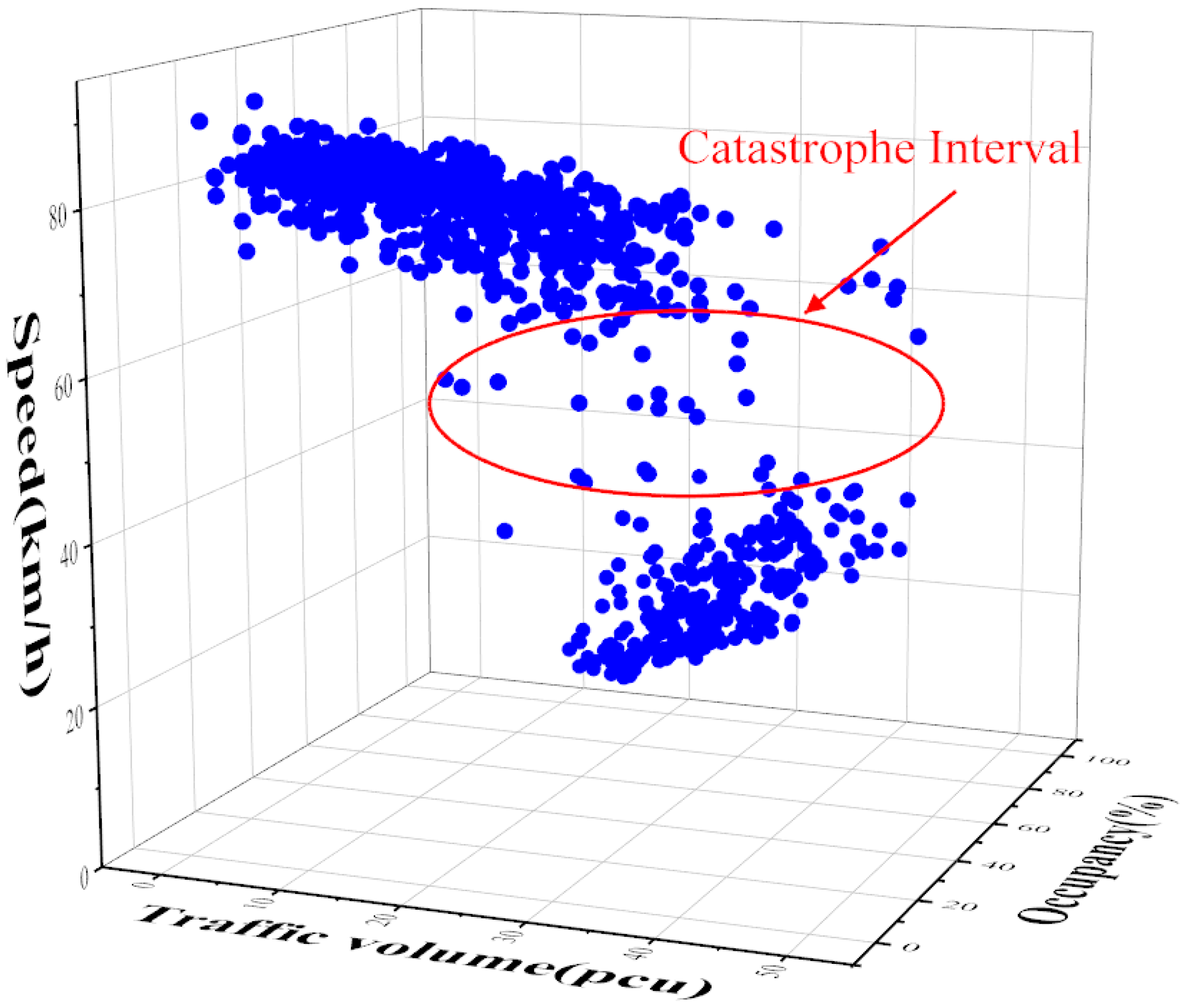
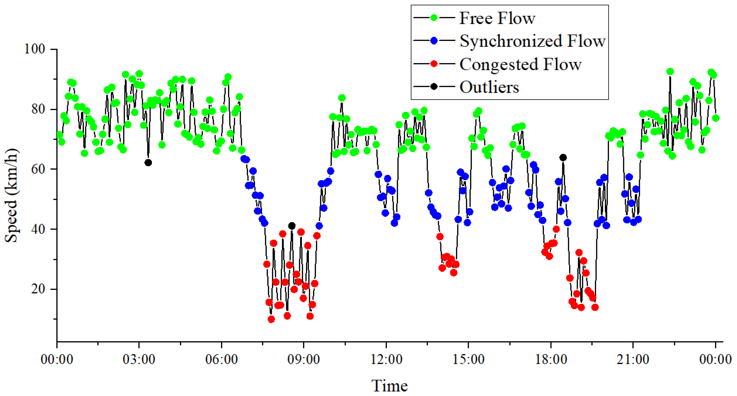
In order to verify whether the simulation platform has high reliability, under the same simulation scenario, detectors were set at the exit, middle, and entrance sections of the weaving area to extract the measured data and simulation data. Then, the measured data of free and congested flow, which are easy to observe, were compared with the simulation results. The validation results of the model are shown in

Table 1. Verification results of simulation model in free flow state.

Detector Number	Measured Speed (km/h)	Simulated Speed (km/h)	Relative Error (%)	Measured Speed (km/h)	Simulated Speed (km/h)	Relative Error (%)
1	69.31	71.13	2.63	1386	1296	6.49
2	70.58	71.52	1.33	1601	1546	3.44
3	68.14	69.96	2.67	1518	1403	7.58
Average value	69.34	70.87	2.21	1502	1415	5.83

and

Table 2. Verification results of simulation model in congested flow state.

Detector Number	Measured Speed (km/h)	Simulated Speed (km/h)	Relative Error (%)	Measured Speed (km/h)	Simulated Speed (km/h)	Relative Error (%)
1	25.94	26.78	3.24	2625	2473	5.79
2	20.13	20.72	2.02	2268	2197	3.13
3	18.63	19.16	2.84	2016	1876	6.94
Average value	21.63	22.22	2.70	2303	2182	5.29

.

From the verification results shown in Table 1 and Table 2, it can be seen that there was little difference between the measured results of speed and traffic volume under different sections and traffic flow conditions and the simulation data. The relative error of all comparison results was no more than 8%. Therefore, using the Vissim simulation platform for traffic simulation is reasonable and reliable. In addition, comparing the relative error values of speed and traffic volume of each section, it can be seen that the relative error in the middle section was the smallest. Moreover, the relative error measured with speed as the index was smaller. Thus, it is more accurate to describe the evolution law of traffic flow with speed as the index in the cusp catastrophe theory model.

Characteristic indicators such as traffic volume, time occupancy rate, and average speed in the middle section of the traffic flow in the weaving section were selected. The relationship between them is shown in Figure 1.

During the evolution of traffic flow, the state of traffic flow exhibited the following characteristics:

(1)

The distribution of traffic flow parameters in free flow and congested flow was relatively concentrated, and the speed change between the two states was discontinuous. The state of traffic flow indicated a catastrophe;

(2)

The speed interval between free flow and congestion flow, i.e., the catastrophe interval, had few data points. In this interval, the traffic flow state changed effortlessly, highlighting the unreachability of the catastrophe interval;

(3)

Under the same traffic volume, there were two different corresponding speeds, and the traffic flow states corresponding to these two speeds were different. There were two steady states of traffic flow, showing a dual modality.

Through the research and analysis of the distribution law of traffic parameters, it can be seen that the traffic flow had prominent catastrophe characteristics, which is highly consistent with the cusp catastrophe theory. Therefore, the cusp catastrophe theory could accurately describe the evolution law of traffic flow.

3. Catastrophe Boundary Extraction with Spectral Clustering Analysis Algorithm

The three-dimensional data after coordinate transformation were projected to the singularity set equation surface, and then we extracted the catastrophe boundary of state variables. The traditional catastrophe boundary extraction method was used to determine the catastrophe length threshold on the basis of experience, and then the interval with minor data points within the variation threshold was identified as the catastrophe interval, which had low confidence and reliability. Machine learning could effectively solve the above problems. Through continuous iteration, the data center was dynamically identified, the traffic flow state was dynamically clustered, the catastrophe boundary was extracted, and the catastrophe interval was determined [25]. The specific process is shown in Figure 2.

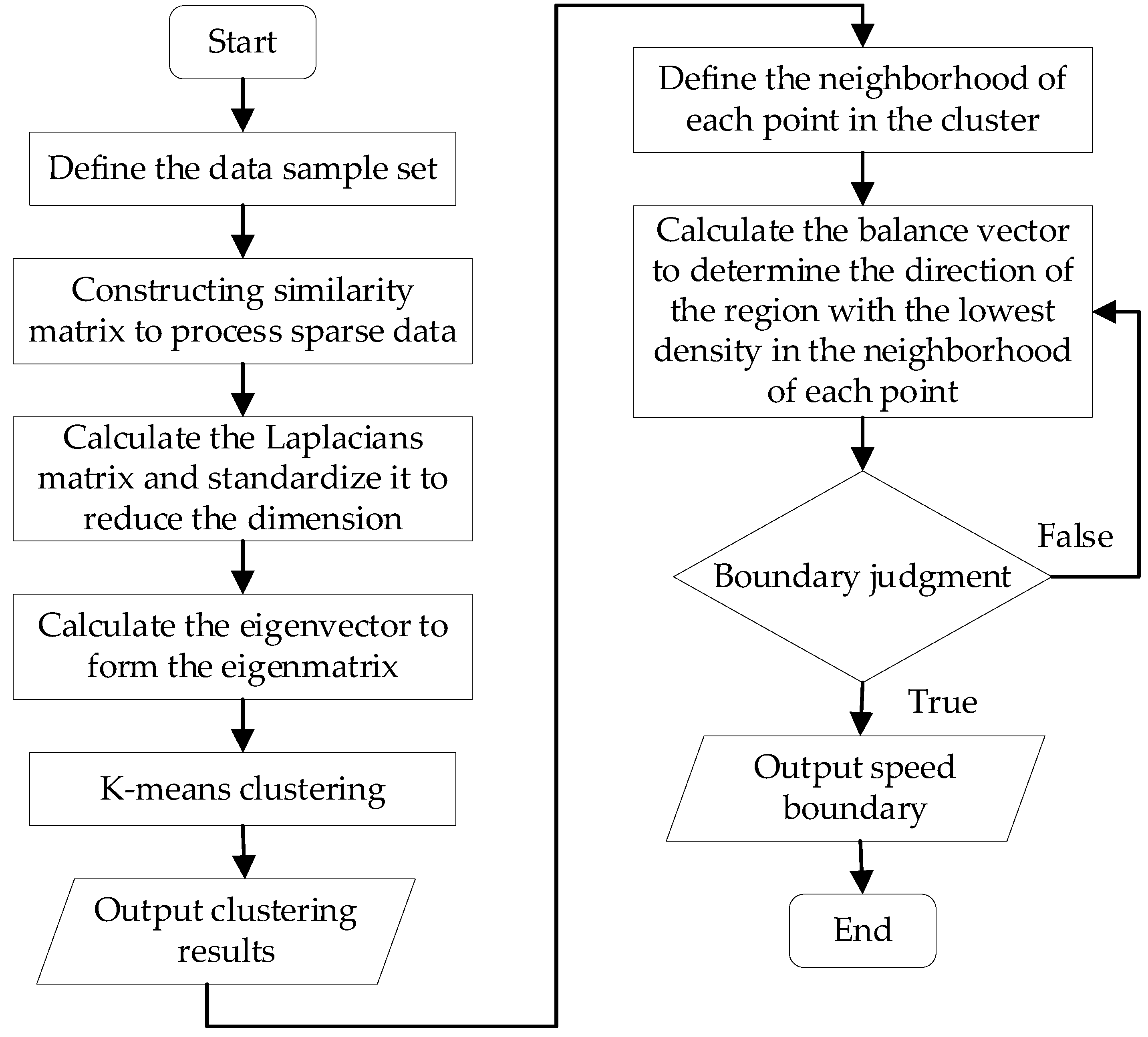
3.1. Analysis of Catastrophe Characteristics of Traffic Flow

As a research hotspot of machine learning, the spectral clustering analysis algorithm can address the inability of traditional dynamic clustering methods to deal with non-spherical cluster data [26,27], cluster traffic flow states efficiently, and provide more accurate and reliable results. The specific process is described below.

(1)

Define the data sample set.

$$X=\left\{x_i|i=1,2,3,\dots ,n\right\},$$

(9)

where $x_i$ is the i-th sample point in the data.

(2)

Take the data to scatter points as an overall network graph, where each scatter point is a node in the network graph, and the connected nodes are edges in the network graph. The similarity between nodes is the weight value of the edge. The similarity calculation formula is as follows:

$${\omega }_{ij}=e^{\frac{-{\Vert x_i-x_j\Vert }^2}{2{\sigma }^2}},$$

(10)

where $\sigma$ is the sample standard deviation, and the value is 0.9.

(3)

Arrange the similarity into a similarity matrix.

$$W=\left\{{\omega }_{ij}|1\le i\le n,1\le j\le n\right\}.$$

(11)

To exclude self-similarity, make the diagonal of matrix w equal to 0.

$$W\left(i,j\right)=0, i=j.$$

(12)

(4)

In order to prevent a single node from being eliminated in the iterative process, a normalized diagonal matrix D is established.

$$D\left(i,i\right)={\displaystyle \sum _{j=1}^N{x}_{ij}}.$$

(13)

(5)

Calculate the Laplacian matrix.

$$L=D^{\frac{1}{2}}W{D}^{\frac{1}{2}}.$$

(14)

(6)

Determine the number of clusters as K; K = 3, representing free flow, synchronized flow, and congested flow. Arrange the vectors with the largest eigenvalues of the first K into the eigenmatrix U.

$$U=\{u_1,u_2,\dots ,u_k\},$$

(15)

where $u_1,u_2,\dots ,u_k$ is the first K eigenvector.

(7)

Normalize the eigenmatrix to get matrix Y.

$$Y_{ij}=\frac{u_{ij}}{\sqrt{{\displaystyle \sum _j{u}_{ij}^2}}}.$$

(16)

(8)

Using each row vector in the matrix Y as a data point, perform clustering through the K-means algorithm, thus obtaining K clustering results $C_1,C_2,\dots ,C_k$.

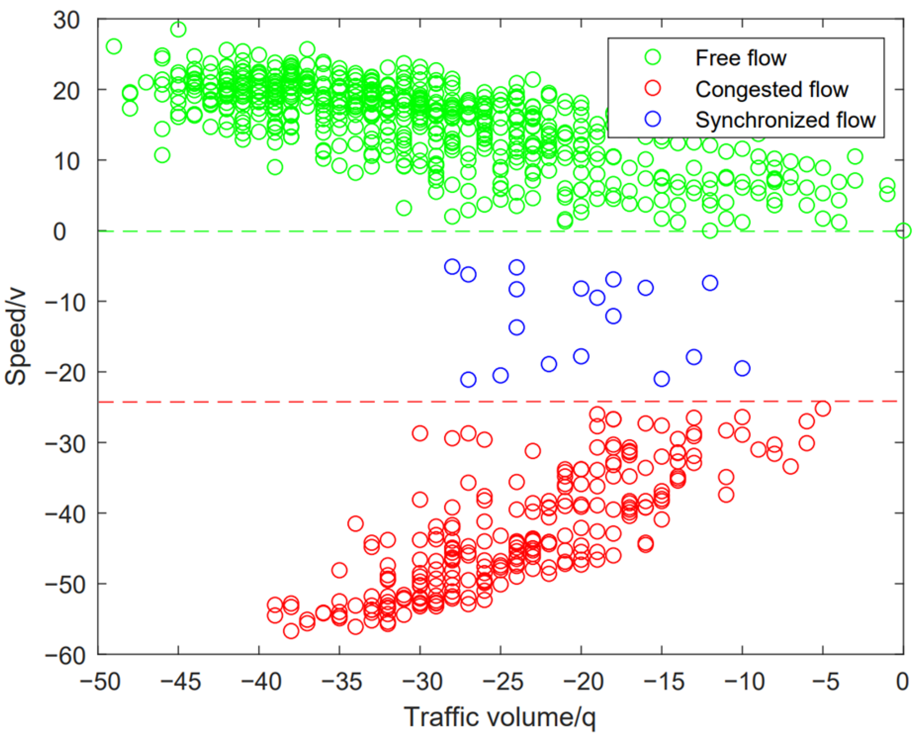
3.2. Clustering Boundary Extraction

In this problem, the catastrophe boundary is the boundary of clustering. The cluster analysis algorithm can effectively classify the data to obtain cluster centers and different types of datasets, but cannot determine the cluster boundary. In order to detect the cluster boundary, the equilibrium vector algorithm is used to extract the catastrophe boundary through iterative discrimination.

For any cluster $C=\left\{x_i|i=1,2,\dots ,m\right\}\subseteq X$, the neighborhood of any point x is $\epsilon \left(x\right)$. From the characterization of clustering results, boundary points are relatively dense points on one side and blank points on the other side, which is especially obvious in catastrophe theory. Therefore, when judging the boundary point, the minimum density direction in the neighborhood $\epsilon$ of the data point can be determined to define the displacement vector as follows:

$$\overrightarrow{v_x}={\displaystyle \sum _{x_i^{\prime }\in \epsilon \left(x\right)}\left(x-x_i^{\prime }\right)}.$$

(17)

Hence, the equilibrium vector of point x is

$$\overrightarrow{b_x}=\{\begin{array}{l}\frac{1}{\Vert \overrightarrow{v_x}\Vert }\overrightarrow{v_x}, \mathrm{if}\Vert \overrightarrow{v_x}\Vert >0\\ \overrightarrow{0}, \mathrm{others}\end{array}.$$

(18)

According to Boolean judgment, the boundary points can be obtained as follows:

$$\mathrm{Boundary}\left(x\right)=\{\begin{array}{l}\mathrm{true} , \mathrm{if} \epsilon \left(x+\rho \overrightarrow{b_x}\right)=\varnothing \mathrm{and} \overrightarrow{b_x}\ne \overrightarrow{0}\\ \mathrm{false} , \mathrm{others}\end{array}.$$

(19)

3.3. Analysis of Traffic Characteristics

The extraction results of the mutation boundary were analyzed, as shown in Figure 3, where green represents the free flow state, red represents the congested flow state, and blue represents the synchronized flow state. It can be seen from the figure that, compared with the free flow state and the congested flow state, the data points of the synchronized flow state were sparser, in line with the catastrophe characteristics of the cusp catastrophe theory. Its catastrophe boundary was [−22.6, 0]. Then, the speed boundary before coordinate transformation was [41.1 km/h, 63.7 km/h].

In order to explore the versatility and universality of the method, several experiments were carried out by changing the parameters of the traffic simulation scenario to obtain the catastrophe boundary of the traffic flow state in different scenarios. The experimental scheme is shown in

Table 3. Summary of experimental scheme.

Experimental Scheme	Experimental Parameters	Initial Value	Final Value	Increment	Remark
1	Weaving volume ratio	0.05	0.35	0.1	Each group of experiments was only carried out according to the initial value, final value, and increment of the group, while the other parameters remained unchanged.
2	Length of weaving section (m)	150	750	150
3	Number of lanes	2	4	1

.

The spectral clustering analysis algorithm was used to extract the speed catastrophe boundary from the data obtained from each simulation experiment, and the relationships between the catastrophe boundary and the weaving volume ratio, the length of weaving section, and the number of lanes were studied.

As shown in Figure 4a, the catastrophe boundary of speed decreased with the increase in weaving volume ratio. When the weaving volume ratio was increased, the vehicles changed lanes more frequently in the weaving section, and the critical speed value of the traffic flow state was lower. With the increase in the length of the weaving section, as shown in Figure 4b, the speed catastrophe boundary showed an upward trend. At this time, vehicles had more lane-changing opportunities during operation, and the traffic flow state had a higher critical speed value. As shown in Figure 4c, when the number of expressway lanes increased, vehicles could change from the outer lane to the inner lane, such that the outer lane had more lane-changing gaps, which improved the speed of traffic flow.

In order to further analyze the sensitivity of various influencing factors to the catastrophe boundary of speed, the change rates of all experimental parameters were drawn as a box plot.

It can be seen in Figure 5 that the weaving volume ratio was more sensitive to the speed catastrophe boundary. The change in weaving volume ratio can affect the traffic efficiency of the mainline and lead to significant changes in the traffic flow state of the weaving section. The length of the weaving section and the number of mainline lanes were less sensitive to the catastrophe boundary of speed. The main reason is that, with the increase in weaving space, the interaction between lanes in the weaving section decreased gradually, and the traffic flow efficiency was higher. The critical speed changed slightly with a slight increase in input traffic volume.

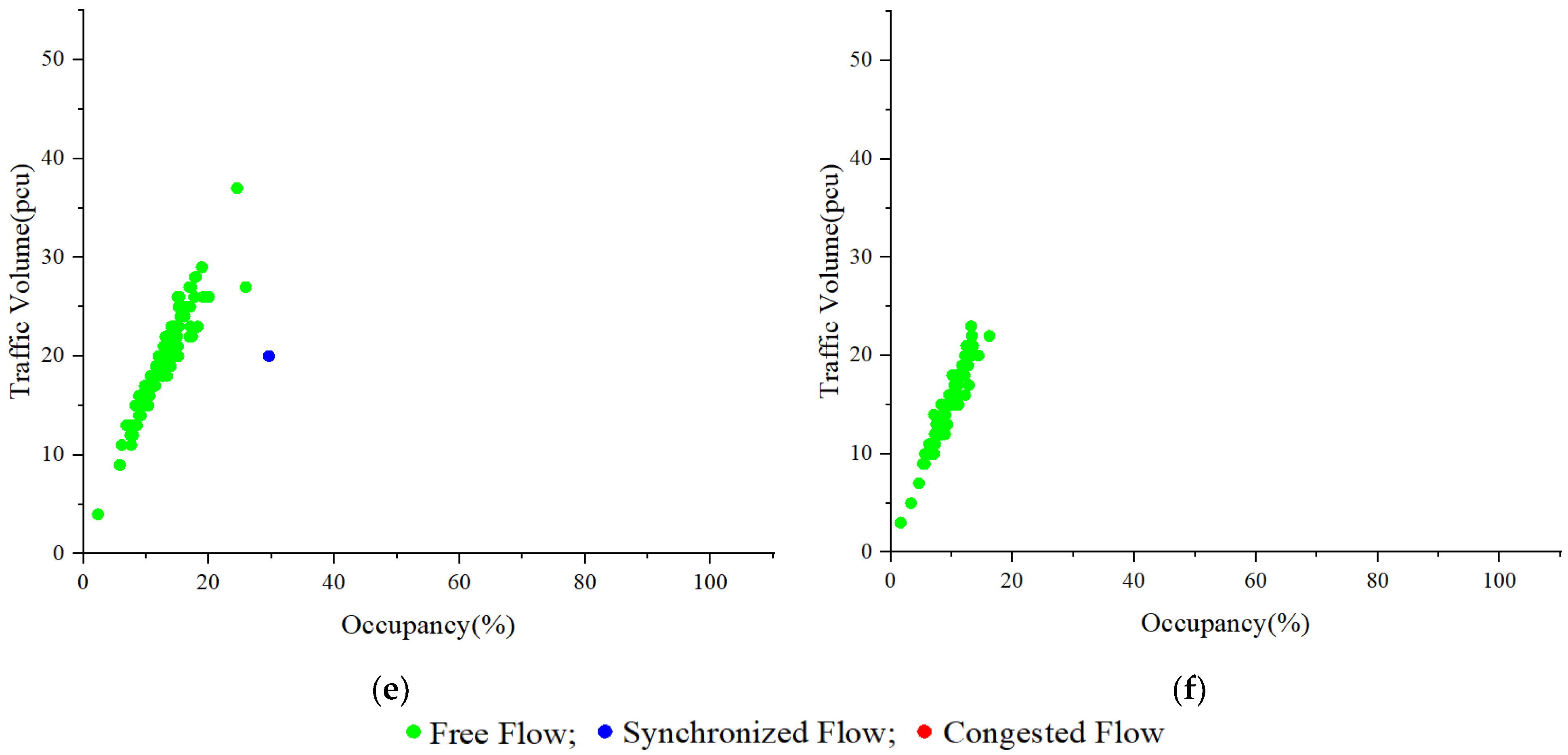
3.4. Example Verification

In order to further verify the evaluation effect of the catastrophe boundary calculation model of traffic state, this paper selected the 24 h speed data measured in the west-to-east direction in the middle of the weaving section of Anshan No. 2 Road, Hang’an Expressway, Qingdao City on 24 November 2021 (Wednesday). Then, time-series graphs of speed parameters were plotted with an interval of 5 min. Finally, according to the speed catastrophe boundary obtained from the simulation data, this paper determined the traffic flow status in each period of the actual expressway weaving section and analyzed the results.

As shown in Figure 6, the evolution of traffic flow state over time was in line with the traffic congestion during the peak period of morning and evening commuting on weekdays. There was a transient synchronized flow state between free flow and congested flow. It can be seen that the extraction method of catastrophe boundary of the traffic flow state based on cusp catastrophe theory is scientific and reasonable for the discrimination results of traffic state in different periods. There were three abnormal values outside of the adjacent data clusters in the state discrimination results, and the accuracy rate was 98.96%. Compared with the neural network algorithm [28] and decision tree algorithm [29] commonly used in traffic state discrimination, improvements of 7.91% and 9.34% were achieved, respectively, indicating good performance.

4. Analysis of Evolution Law of Traffic Flow State

4.1. Formation Law of Traffic Flow Congestion

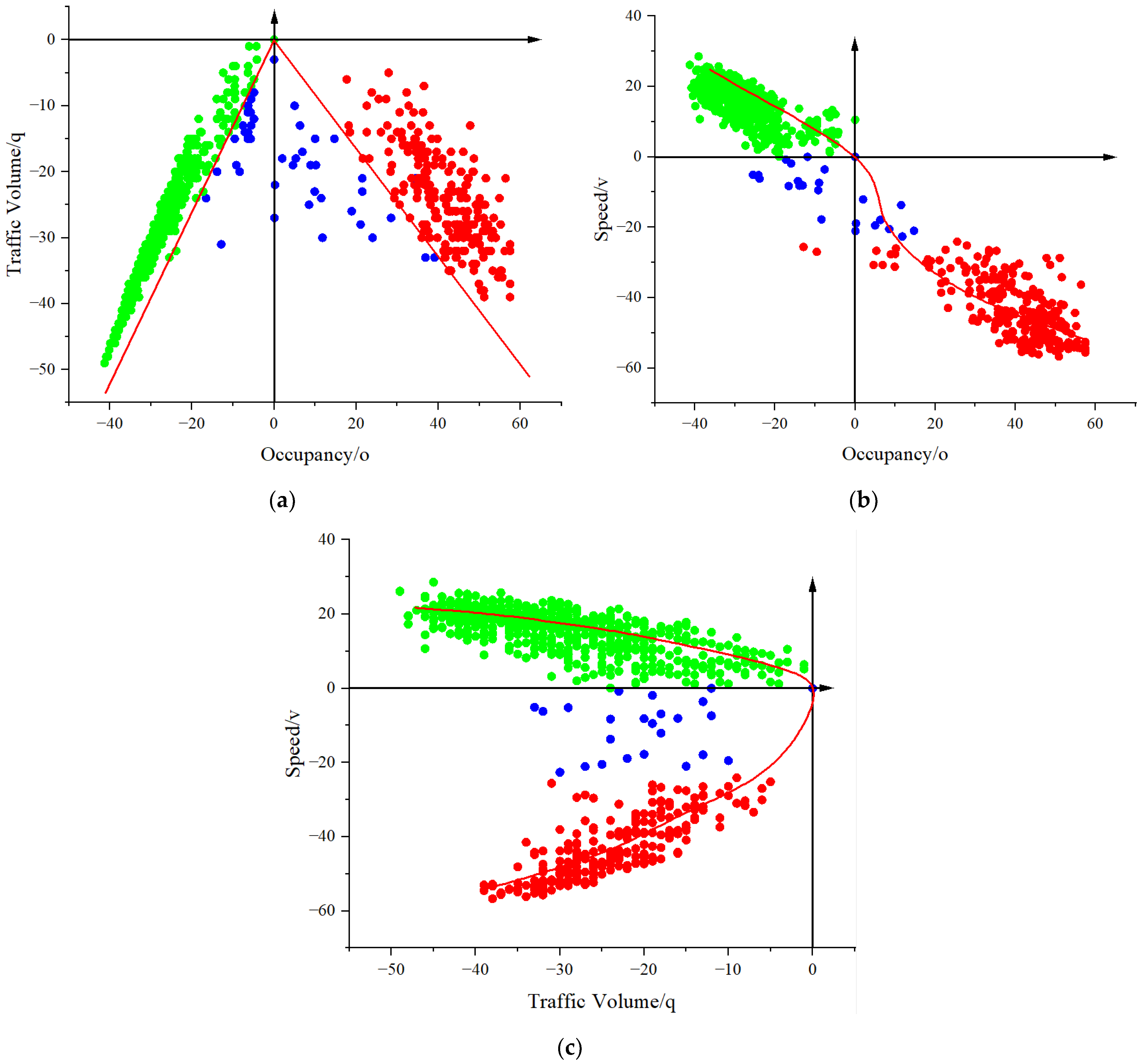
The equilibrium surface diagram of cusp catastrophe theory was analyzed. As shown in Figure 7, the system had a dual modality. The traffic flow had two steady states, free flow and congested flow, in the upper and lower lobes of the equilibrium surface, respectively. The region characterized by surface folds was unstable, i.e., a synchronized flow state, which could be either continuous or discontinuous, indicating an unattainable stable state, which could jump to the upper lobe or the lower lobe. Thus, the synchronized flow state can evolve into a congestion or a free-flow state in a traffic flow system. When the traffic flow evolves from free to congestion, the speed evolves from point A to point B and then catastrophically to point B₁. In the process of congestion dissipation, the speed evolves catastrophically from point C to point C₁, indicating that the catastrophe of the system has hysteresis. The point where the surface folds disappear is the coordinate origin of the equilibrium surface. At this time, the traffic volume, occupancy, and speed after data transformation are 0, corresponding to the maximum traffic volume, critical occupancy, and optimal speed of the original data.

The equilibrium surface plot of cusp catastrophe theory was projected onto three planes for analysis.

(1)

Analysis of the relationship between traffic volume and occupancy

In the cusp catastrophe model, the bifurcation set equation for traffic volume and occupancy can be obtained by eliminating V. It is crucial to study the two-state potential and situation catastrophe using cusp catastrophe theory. Figure 8a shows that the traffic volume was distributed in the second and third quadrants, with the free flow on the left and the congested flow on the right. There was a prominent bifurcation area in the middle, indicating synchronous flow. In the free flow state, the time occupancy increased with traffic volume, and the traffic volume reached the maximum at the origin. Then, the traffic flow fell into the synchronous flow state. In the synchronous flow state, the traffic flow had a lower occupancy rate than the free flow, but the traffic volume was not as large. Subsequently, with the continuous input of vehicles, the occupancy increased, the traffic volume decreased gradually, and the traffic flow entered the state of congestion.

(2)

Analysis of the relationship between speed and occupancy

In the process of traffic flow operation, as shown in Figure 8b, the system state was in the upper leaf of the equilibrium surface. That is, the vehicle flow speed was in the free flow state. When it gradually approached the origin, the occupancy increased gradually, and the change process of the state was continuous. Upon reaching the origin, a slight change in the control variable would result in the velocity jumping to the lower leaf of the equilibrium surface at the origin, thereby suddenly changing the speed. Upon increasing the occupancy, the system state was stable in the lower half of the leaf, i.e., the congested flow state.

(3)

Analysis of the relationship between speed and traffic volume

The cusp catastrophe model could obtain the singular point set equation of traffic volume and speed by deriving the equilibrium surface equation. As shown in Figure 8c, when the traffic flow was in the free flow state, the speed was in the upper leaf of the system. At this time, the vehicles traveled at the desired speed. When the traffic volume increased, the speed decreased smoothly, but the decrease was not significant until reaching the singularity, at which point the speed reached the optimal speed. This resulted in a speed catastrophe, which reached the congestion state via the synchronous flow state, and the speed and traffic volume decreased simultaneously.

4.2. Dissipation Law of Traffic Flow Congestion

Congestion dissipation is an essential process in the evolution of traffic flow, and its law is the primary basis for studying dissipation control strategies. In order to explore the dissipation law of traffic flow congestion, the input traffic volume was set as 4000–1500 pcu/h, and the simulation data of the intermediate section for a total of 6 h were selected as the research object. The results are shown in Figure 9.

Figure 9a–f show the distribution relationships between traffic volume and occupancy rate collected in each period (1 h). As shown in Figure 9a, at the beginning of the simulation, only a few vehicles were in the free flow state, before quickly entering the congestion state due to a speed catastrophe. Almost all the traffic volume was distributed in the congestion flow area. Then, with the decrease in input traffic volume, as shown in Figure 9b, the traffic flow congestion was alleviated; however, most vehicles were still in the congested flow state, with a few vehicles reaching the free flow state. With a further reduction in the input traffic volume, as shown in Figure 9c, traffic volume and occupancy distribution returned to the average level, and most of the traffic volume was in the free flow state. Then, with the continuous reduction in the input traffic volume, the traffic flow state was further optimized until Figure 9f, where the traffic flow distribution was entirely in the free flow state.

Comparing Figure 9b,c, it can be seen that, during the process of congestion dissipation, the distribution of traffic volume changed significantly, indicating that the catastrophe of the traffic flow state would still occur. There was a noticeable data gap between the two steady states of congested flow and free flow, indicating the synchronized flow region. There were very few data points in this region, verifying the inaccessibility of the cusp catastrophe theory. At the same time, comparing the evolution law of congestion formation, it can be seen that the two parameters of traffic volume and occupancy were generally consistent before congestion formation and after congestion dissipation. However, the traffic volume and occupancy during system catastrophe were different, highlighting the hysteresis of cusp catastrophe theory.

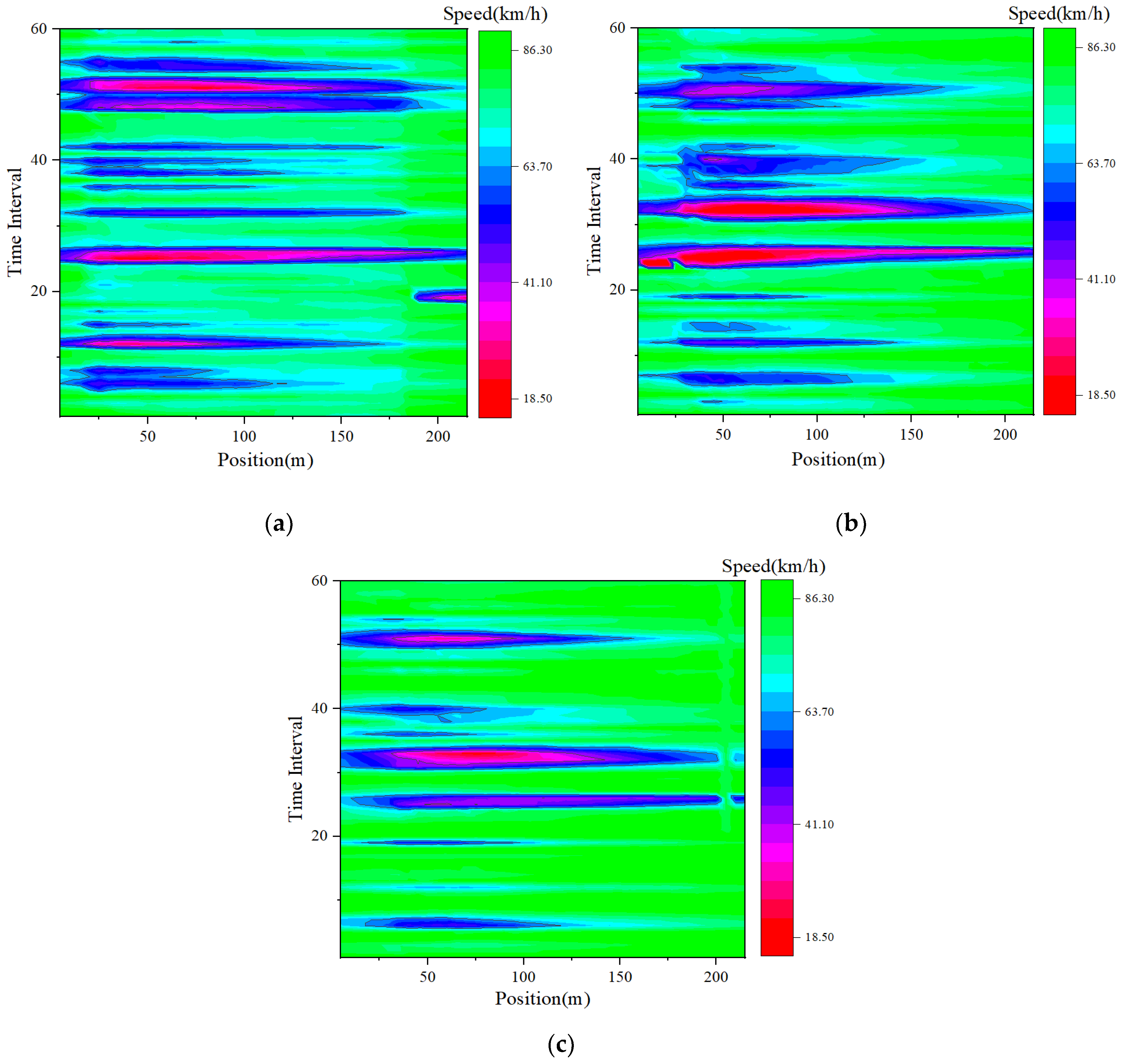
4.3. Temporal and Spatial Evolution Characteristics of Traffic Flow State

When the input traffic volume was 3000 pcu/h, the average speed of the cross-sections at all positions of the outer, middle, and inner lanes was selected as the research object. On the basis of the cusp catastrophe theory, the evolution law of the formation and dissipation of urban expressway traffic congestion and its internal mechanism were studied in terms of space and time.

In Figure 10, the green area is free flow, the red area is congested flow, and the blue area is synchronized flow with a speed catastrophe. As shown in Figure 10a, there were 13 speed catastrophes in the outer lane during the temporal simulation, of which eight did not evolve into congested flow but re-evolved into free flow, whereas five evolved into congested flow. Furthermore, the synchronized flow area was narrow, in accordance with the characteristics of the cusp catastrophe. In the spatial simulation, four of the five congestion events occurred at 10 m, near the exit of the weaving section, whereas one occurred at 190 m, near the entrance of the weaving section. Moreover, the speed catastrophe positions of the remaining eight events did not evolve into congestion flow, consistent with their location. As shown in Figure 10b, 13 speed catastrophes also occurred in the middle lane during the temporal simulation, of which four evolved into congested flow and nine re-evolved into free flow. Spatially, all four congestion events occurred near 10 m, i.e., near the exit of the weaving section. For the inner lane, as shown in Figure 10c, there were nine speed catastrophes during the temporal simulation, of which three evolved into the congested flow state, which is a better outcome than the outer and middle lanes. Spatially, the congestion position was also near the exit of the weaving section.

The causes of congestion according to the temporal and spatial distribution of traffic flow are analyzed below.

(1)

For the outer lane, the traffic flow at the entrance of the weaving section evolved into traffic congestion only once. This is because most vehicles could find a gap to freely change lanes during the acceleration process in the weaving lane. These vehicles did not have much impact on the overall traffic flow. Only a few vehicles forcibly changed lanes to enter the mainline when vehicle acceleration was not completed and a gap was not found. This resulted in a traffic flow speed catastrophe, forming a bottleneck in the entrance area. When conservative traffic participants do not find a gap during driving in the weaving lane, they continue to drive in this lane until the exit, before stopping and waiting on the opportunity to change lanes. This results in a traffic flow speed catastrophe, causing congestion at the exit.

(2)

For the middle lane, since the continuous lane-changing of an entry vehicle into the inner lane rarely occurs after entering the weaving section, there was no congestion near the entrance during the simulation. In the vicinity of the exit, some vehicles in the weaving lane changed lanes into the outer lane, while some vehicles in the outer lane intended to change lanes inward. Thus, some vehicles in the inner lane made a forced lane change near the exit without a suitable gap, thus hindering traffic flow in the middle lane. Therefore, there were more speed catastrophes near the exit in the middle lane than in the outer lane. Moreover, in the congested state, due to the joint obstruction of the outer lane and the inner lane, the congestion in the middle lane lasted longer, and the congestion dissipated more slowly.

(3)

For the inner lane, similar to the middle lane, no vehicle was forced to change lanes continuously to enter the inner lane without finding a gap during the simulation; hence, there was no speed catastrophe near the entrance. When the traffic volume is too large, vehicles in the inner lane trying to exit the expressway stop near the exit and wait for a lane change, which affects the upstream traffic flow and leads to a speed catastrophe near the exit. However, the inner lane is less affected by the outer lane and middle lane; in most cases, it is only affected by vehicles leaving the lane. Therefore, its traffic flow is smoother than the other two lanes, and there are fewer speed disasters and congestion events.

(4)

When the structure of the weaving section changes, such as the length of the weaving section and the number of expressway lanes, the evolution trend of traffic flow will not change. However, when the space in the weaving section is increased, the vehicles have more sufficient lane change gaps, the traffic flow has higher efficiency, and the number of traffic jams is decreased. Similarly, when the length of the weaving section and the number of lanes are reduced, the number of traffic jams and the duration of congestion are increased.

5. Conclusions

This study showed that the urban expressway, as a transportation hub bearing most of the pressure of the urban road network, and the congestion of its traffic flow affect the efficiency of the entire urban road network. The evolution law of the expressway traffic flow state is key to formulating the congestion control scheme and studying the congestion dissipation strategy. We used the traffic simulation platform Vissim to simulate the operation of expressway traffic flow and extract its characteristic parameters; on this basis, we determined their influence on the state evolution law of expressway traffic flow.

(1)

In the evolution process of traffic flow state, there are two relatively stable traffic flow states: free flow and congested flow. There are apparent crack areas between the two traffic flow states, indicating a catastrophe in the evolution process of traffic flow.

(2)

Spectral clustering analysis algorithm can address the inability of the traditional clustering algorithm to deal with non-spherical cluster data and effectively extract the catastrophe boundary of traffic flow according to the node similarity of the network graph. The accuracy achieved in this study was 98.96%.

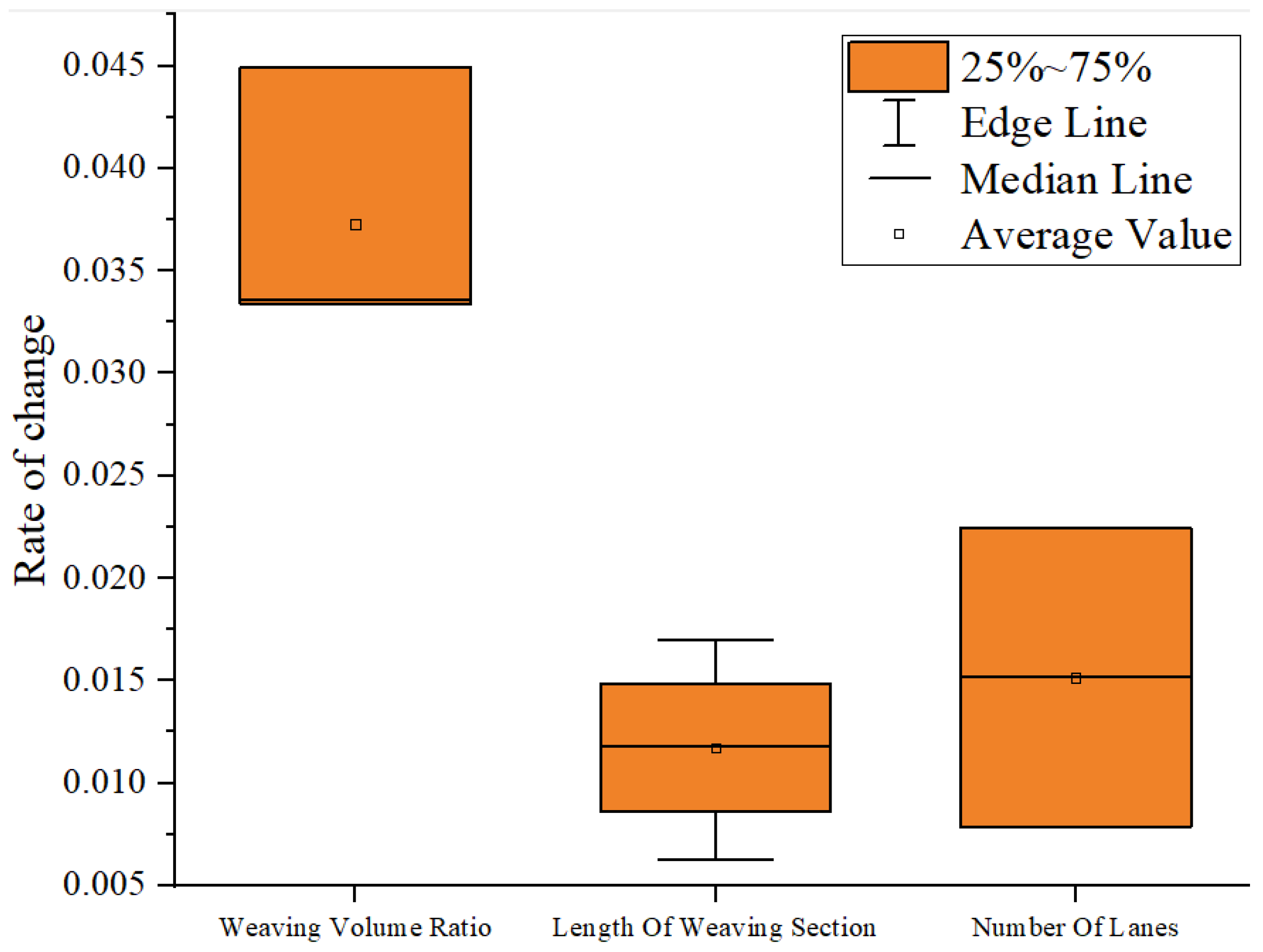
(3)

The catastrophe boundary of the traffic flow state is affected by many factors, among which the weaving volume ratio is the most sensitive.

(4)

In the formation and dissipation of traffic congestion, speed catastrophes will occur, but the corresponding traffic volume is different in the two cases.

(5)

This study only analyzed the internal causes of the evolution law of congestion formation and dissipation in a single weaving section. It did not consider external factors such as congestion in related road sections, which can be investigated in a future study.

References

1. Greenshields, B.D. A Study of Traffic Capacity. Highw. Res. Board Proc. 1935, 14, 448–477. [Google Scholar]
2. Lighthill, M.J.; Whitham, G.B. On Kinematic Waves II. A Theory of Traffic Flow on Long Crowded Roads. Proc. R. Soc. London. Ser. A. Math. Phys. Sci. 1955, 229, 317–345. [Google Scholar]
3. Richards, P.I. Shock Waves on the High way. Oper. Res. 1956, 4, 42–51. [Google Scholar] [CrossRef]
4. Hao, J.; Qu, D.Y.; Zhang, J.L.; Guo, T.; Wang, H. Analysis method of traffic flow characteristics based on molecular dynamics. J. Qingdao Technol. Univ. 2013, 34, 87–91, 124. [Google Scholar]
5. Zhang, B.; Zhao, H.Y. Parameter correlation analysis and research on single-lane cellular automaton NS model. J. Kunming Univ. Sci. Technol. 2016, 41, 45–51. [Google Scholar]
6. Wang, Y.; Chu, X.; Zhou, C.; Jia, B.; Lin, S.; Wu, Z.; Zhu, H.; Gao, Z. Evolvement law of a macroscopic traffic model accounting for density-dependent relaxation time. Mod. Phys. Lett. B 2017, 31, 1750291. [Google Scholar] [CrossRef]
7. Hattam, L. Travelling wave solutions of the perturbed mKdV equation that represent traffic congestion. Wave Motion 2018, 79, 57–72. [Google Scholar] [CrossRef] [Green Version]
8. Younes, M.B.; Boukerche, A. A performance evaluation of an efficient traffic congestion detection protocol (ECODE) for intelligent transportation systems. Ad Hoc Netw. 2015, 24, 317–336. [Google Scholar] [CrossRef]
9. Fei, W.P.; Song, G.H.; Zhang, F.; Gao, Y.; Yu, L. Practical approach to determining traffic congestion propagation boundary due to traffic incidents. J. Cent. South Univ. 2017, 24, 413–422. [Google Scholar] [CrossRef]
10. Li, S.B.; Fu, B.B.; Sun, T.; Dang, W. Research on complex network mesoscopic traffic flow with dynamic limit speed control strategies. Complex Syst. Complex. Sci. 2017, 14, 32–42. [Google Scholar]
11. Hu, J.R.; He, L. Freeway traffic flow condition criterion method based on cusp catastrophe theory. China J. Highw. Transp. 2017, 30, 137–144. [Google Scholar]
12. Ghadami, A.; Epureanu, B.I. Forecasting the Onset of Traffic Congestions on Circular Roads. IEEE Trans. Intell. Transp. Syst. 2020, 22, 1196–1205. [Google Scholar] [CrossRef]
13. Shao, Z.Y.; Zhang, L.; Wu, H. Evolution of urban traffic state based on cusp catastrophe. J. North China Univ. Sci. Technol. 2021, 43, 74–80. [Google Scholar]
14. Chaurasia, B.K.; Manjoro, W.S.; Dhakar, M. Traffic congestion identification and reduction. Wirel. Pers. Commun. 2020, 114, 1267–1286. [Google Scholar] [CrossRef]
15. Lin, L.; Chen, J.; Qu, D.Y.; Hei, K.; Han, L.; Bing, Q. Study on traffic state identification method based on K-means clustering algorithm. J. Qingdao Technol. Univ. 2019, 40, 109–114. [Google Scholar]
16. Liu, C.M.; Juang, J.C. Estimation of Lane-Level Traffic Flow Using a Deep Learning Technique. Appl. Sci. 2021, 11, 5619. [Google Scholar] [CrossRef]
17. Gao, C.; Wang, J.F.; Lu, X.; Chen, X. Urban Traffic Congestion State Recognition Supporting Algorithm Research on Vehicle Wireless Positioning in Vehicle–Road Cooperative Environment. Appl. Sci. 2022, 12, 770. [Google Scholar] [CrossRef]
18. Thom, R. Catastrophe theory. Nature 1977, 270, 658. [Google Scholar] [CrossRef] [Green Version]
19. Navin, F.P.D. Traffic congestion catastrophes. Transp. Plan. Technol. 1986, 11, 19–25. [Google Scholar] [CrossRef]
20. Huang, Y.G.; Zhang, H.M.; Liu, H.J.; Zhang, S. An Analysis of the Catastrophe Model and Catastrophe Characteristics of Traffic Flow Based on Cusp Catastrophe Theory. J. Adv. Transp. 2022, 2022, 2837338. [Google Scholar] [CrossRef]
21. Zeng, J.W.; Qian, Y.S.; Yu, S.B.; Wei, X.T. Research on critical characteristics of highway traffic flow based on three phase traffic theory. Phys. A Stat. Mech. Its Appl. 2019, 530, 121567. [Google Scholar] [CrossRef]
22. Hall, F.L. An interpretation of speed-flow-concentration relationships using catastrophe theory. Transp. Res. Part A Gen. 1987, 21, 191–201. [Google Scholar] [CrossRef]
23. Herrera, J.C.; Work, D.B.; Herring, R.; Ban, X.J.; Jacobson, Q.; Bayen, A.M. Evaluation of traffic data obtained via GPS-enabled mobile phones: The Mobile Century field experiment. Transp. Res. Part C 2010, 18, 568–583. [Google Scholar] [CrossRef] [Green Version]
24. Carli, R.; Dotoli, M.; Epicoco, N.; Angelico, B.; Vinciullo, A. Automated Evaluation of Urban Traffic Congestion Using Bus as a Probe. In Proceedings of the IEEE International Conference on Automation Science & Engineering, Gothenburg, Sweden, 24–28 August 2015; pp. 967–972. [Google Scholar]
25. Filipovska, M.; Mahmassani, H.S. Traffic Flow Breakdown Prediction using Machine Learning Approaches. Transp. Res. Rec. J. Transp. Res. Board 2020, 2674, 560–570. [Google Scholar] [CrossRef]
26. Yang, S.Y.; Wu, J.P.; Qi, G.Q.; Tian, K. Analysis of traffic state variation patterns for urban road network based on spectral clustering. Adv. Mech. Eng. 2017, 9, 1687814017723790. [Google Scholar] [CrossRef]
27. Geng, Y.L.A. Research on Clustering Algorithm for Clusters with Irregular Structure; Beijing Jiaotong University: Beijing, China, 2021. [Google Scholar]
28. Wu, W.T.; Jin, W.Z.; Lin, P.Q. The method of traffic state identification based on BP neural network. J. Transp. Inf. Saf. 2011, 29, 71–74. [Google Scholar]
29. Fang, L.X.; Wei, L.Y.; Yan, W.Y. Prediction of traffic congestion based on decision tree. J. Hebei Univ. Technol. 2011, 29, 71–74. [Google Scholar]
Figure 1. Data of traffic flow according to simulation.
Applsci 12 06291 g001
Figure 2. Flow chart of the method for extracting the catastrophe boundary of speed.
Applsci 12 06291 g002
Figure 3. Extraction results of catastrophe boundary.
Applsci 12 06291 g003
Figure 4. Speed catastrophe boundary in different scenarios. (a) Weaving volume ratio—catastrophe boundary; (b) Length of weaving section—catastrophe boundary; (c) Number of lanes—catastrophe boundary.
Applsci 12 06291 g004aApplsci 12 06291 g004b
Figure 5. Sensitivity of speed catastrophe boundary based on all parameters.
Applsci 12 06291 g005
Figure 6. Discrimination results of traffic state in the weaving section of Hang’an Expressway.
Applsci 12 06291 g006
Figure 7. Equilibrium surface of cusp catastrophe theory.
Applsci 12 06291 g007
Figure 8. Distribution of traffic flow parameters in cusp catastrophe model. (a) Traffic volume—occupancy distribution; (b) Speed—occupancy distribution; (c) Speed—traffic volume distribution.
Applsci 12 06291 g008
Figure 9. Distribution of traffic volume as a function of occupancy during congestion dissipation. (a) 0–1 h; (b) 1–2 h; (c) 2–3 h; (d) 3–4 h; (e) 4–5 h; (f) 5–6 h.
Applsci 12 06291 g009aApplsci 12 06291 g009b
Figure 10. Temporal and spatial distributions of traffic flow state. (a) Outer lane; (b) Middle lane; (c) Inner lane.
Applsci 12 06291 g010