Morphometric-hydro Characterization of the Coastal Line between El-Qussier and Marsa-Alam, Egypt: Preliminary Flood Risk Signatures

Abstract

Egypt is highly exposed to flash flood hazards, particularly in Sinai Peninsula and along the Red Sea coast, causing sudden and huge damages to constructions and huge losses in human lives during a very short time. This paper investigates the dominant characterization of morphometrical features and their relationships with the hydrological behaviors along an important strip of the western Red Sea coast. The study focuses on analyzing the October 2009 and 2019 storm events along the coastal area between EL-Qussier and Marsa Alam in order to intiate a preliminary flood risk assessment model. Morphometric features along the entire study zone provide a complete scenario of the nature of the catchments and sub-catchments development. Numerous morphometric indexes such as catchments geometry, areal indexes, linear indexes, and relief indexes were examined through processing different sets of data. Modern techniques such as remote sensing and geospatial analysis were applied to process different spatial and spectral data. The hydrological model (HEC-HMS) in the WMS software was run to delineate the catchments and sub-catchments and extract the peak flow hydrograph curves for the main catchments. The results of the water amounts and peak flow were calculated using the SCS unit hydrograph approach. The hydrological characteristics of the major catchments reveal conditions for moderate levels of flash flooding. The study ended with a number of recommendations that could minimize the negative effects of the flash flood hazards.

1. Introduction

Natural hazards such as earthquakes and tsunamis can be described as sudden events that cause loss of life, widespread property destruction, and huge negative effects on the civilization and population. During the last 70 years, more than 11,000 disasters triggered by natural hazards have been monitored and recorded [1]. Climate-related hazard risks represent nearly over two-thirds of natural hazards deaths [2,3,4]. Their effects increased from 76% in the 1960s to 83% during the past decade [1]. Floods are one of the most common and dangerous climate-related natural hazards. They harm more humans globally each year than any other disaster. Storm events or excessive amounts of water reservoir are the main causes of flash flooding [5]. About 44% of the deaths by natural hazards are directly due to surface runoff (flash floods) [6,7]. According to the International Disaster Database (EM-DAT, 2020; https://www.emdat.be/ (accessed on 16 May 2022)), 46% of natural hazards were floods that affected more than 673 million population between 2010 and 2019. Worldwide, extensive efforts are applied to minimize or cope with the negative effects of this phenomenon; nevertheless, flash floods are occurring periodically, causing serious property destruction, serious loss of life, and huge economic damages [8,9]. During the last 4 decades, flash flooding hazards have caused nearly 2466 fatalities in Europe, while only 458 fatalities were recorded in the Mediterranean regions [10]. Arid and semi-arid regions were hit by the negative effects of flash flooding events as well. For example, catastrophic floods attacked Jordin in March 1966, which destroyed Ma’an City and caused around 200 deaths and 250 serious injuries [7,8]. In Egypt, Sinai Peninsula was battered on the 17 and 18 January 2010 by a flash flood that led to many deaths, injuries, and missing people [11]. During the last 5 years in Saudi Arabia, more than 10,000 houses have been damaged, in addition to 113 deaths because of flood events [12].

Investigation of geological hazards and monitoring their serious impacts on the environment requires comprehensive geo-information and continuous earth observations. Processing of high spatial resolution data through geospatial analysis is a very powerful technology to expand our understanding of the nature of geological landscape developments and geological hazards and aids in investigating the variations in tectonic activity and geological hazards mitigations, particularly along seismically active regions [13,14,15,16]. For example, authors in ref. [14] calculated different morphotectonic indexes to examine the tectonic signals in the Carpathian mountain massif region in Poland. In addition, seismic hazards assessment of active spots was examined by many researchers [17,18,19], while others applied the advanced tools to provide insight into the analysis of geological hazards in arid regions [20,21]. For example, authors in ref. [18] attempted to assess the tectonic activity of Mikir massif in India, and they modelled an assessment for irrigation and hydropower development of the study area; on the other hand, authors in ref. [20] established a hydraulic and hydrologic model for the Ayamama River in Turkey. Using GIS technique to generate digital elevation models (DEMs) and extract watersheds and drainage systems is one of the most effective methods in the geospatial technologies [22,23]. The remote sensing technique has provided temporal and spatial information for more accurate monitoring. Applied these recent techniques, coupled with geomorphological and hydrological data is very effective in assessing, categorizing, and analyzing the collected data in order to assess the different flash floods [9]. The work of [9] studied the flood risk assessment in a metropolitan urban city in Greece using GIS technology, and the authors modeled the distribution of the hazard spots. Morphometric and hydrological parameters are widely used in exploring the catchments’ geomorphic history and development of their drainage network [5,10]. For example, Youssef et al. [8], examined the safety of one of the most important monument roads in Egypt. They applied GIS on remotely sensed data to estimate the flash flood hazard level and developed models to trace the flood hazards in highway areas. Morphometric and hydrological parameters aid in understanding the variation in the hydrological characteristics of the related sub-catchments [20,21].

The main objective of this study is to expand the current literature to include flood mitigation strategies between the El-Qussier and Marsa-Alam coastal region, which has no sufficient flooding studies. The data found in this study were processed and analyzed to calculate the effective morphometric parameters along the main catchments and sub-catchments in order to assess the risk of flash floods that periodically occur. For these objectives, we applied remote sensing and geospatial technologies for morphometric landforms extraction and analysis. In addition, it aims to evaluate two major flooding events to quantify surface water using the Hydrologic Engineering Center’s Hydrologic Modeling System (HEC-HMS) and Soil Conservation Service (SCS) unit hydrograph model. Generally, this study aims to fill a geo-hazard studies gap along an important coastal zone of the Egyptian Red Sea coast.

2. Study Area

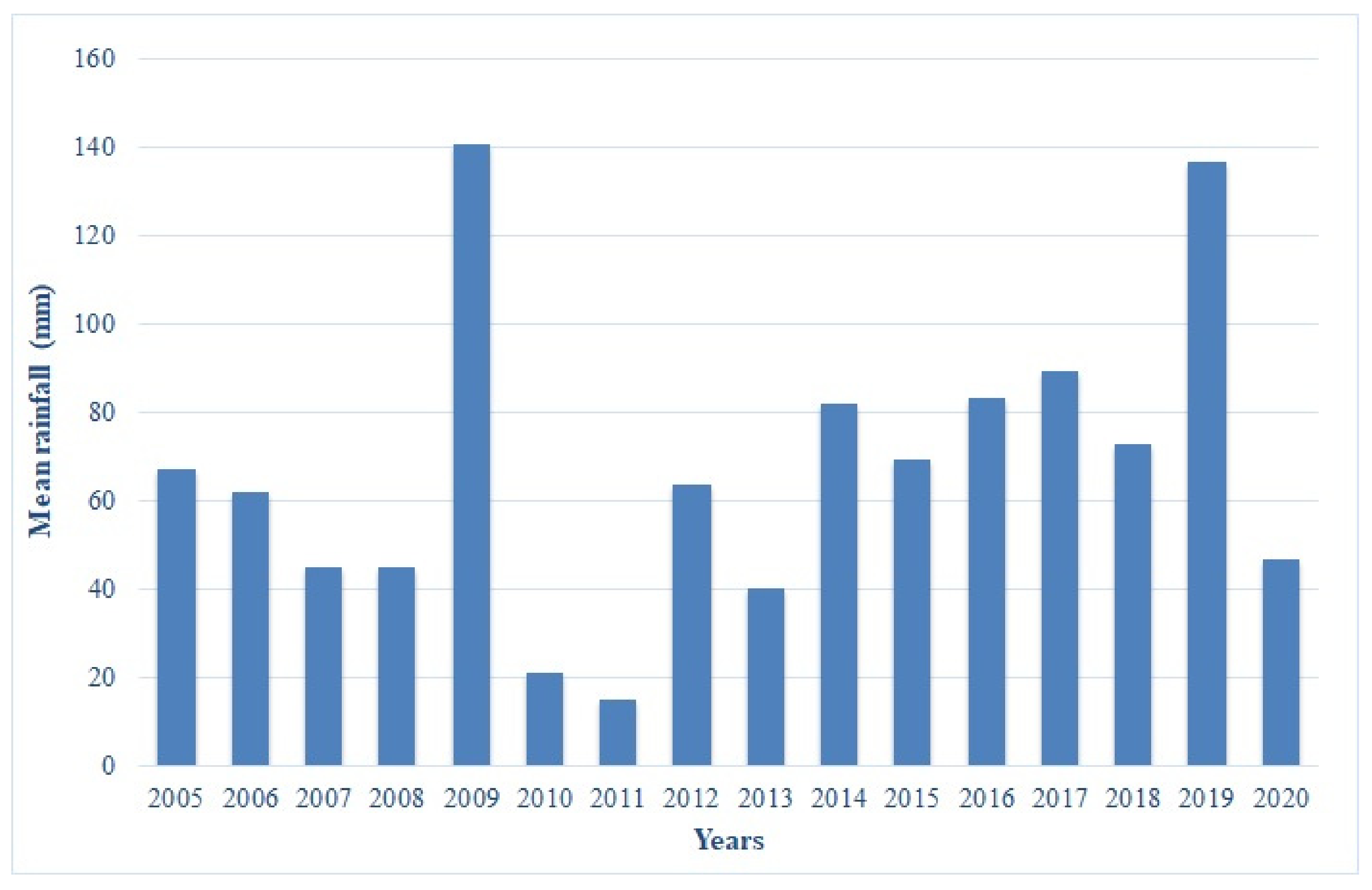
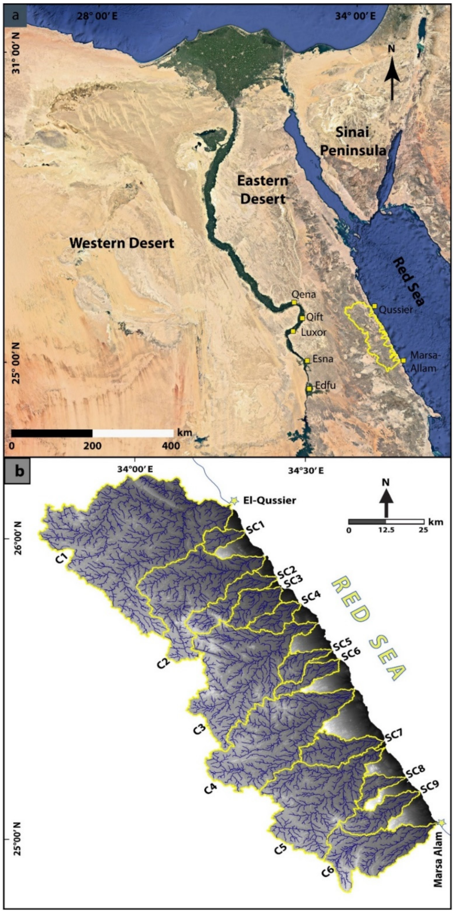
2.1. Description of the Research Area

The Egyptian Red Sea Coast is characterized by a long history of flash flooding catastrophes. On 27 and 28 October 2016, huge flash flood hit Ras Gharib City on the Red Sea coast and extended to cover some cities along the Nile River, it causes many deaths and injuries [21,24]. In October 2019, floods attacked the new Cairo City inside the capital of Egypt and caused 11 deaths and significant property damage [21]. This flood was reported as the most significant event during the last 50 years in terms of rising rates [25]. This flooding events started in August and increased in October, with a very intense rainfall rate [25]. In Lake Nasser, the water level has reached the highest level in comparison to the previous 50 years [25]. During the same year, particularly on November 14, heavy floods hit south Marsa Alam City in addition to Abu Ghosun village [21]. Extensive hydrological and flash floods assessments were applied with a focus on the Red Sea coast using different materials and techniques, e.g., [21,26,27]. Furthermore, in 2009, the first early flood warning system was installed in Egypt. This system contains different models for rainfall–runoff modeling, rainfall forecasting, and hydraulic modeling [25]. Egypt and its eastern desert reflect a large amount of sunshine, which averaged 3530 h in the long-term [28]. The average maximum temperature reaches 35 °C during July and August, while it could decreases to 10 °C in January and February [25]. The annual humidity ranges between 71% in summer and 53% in the wintertime [25]. Particularly, the Red Sea coastal line is characterized by strong winds that come from northwest regions [28]. In Hurghada region, the wind speed was estimated to be recorded at 5.5 m/s [25,28]. The weather conditions data of the study area were collected from Data Access Viewer-NASA POWER (https://power.larc.nasa.gov/data-access-viewer/ (accessed on 16 May 2022)) in 2009 and 2019, respectively. It reflects 39.19% and 38.28% of humidity, 3.35 m/s and 3.84 m/s of wind speed, and 27.95 °C and 28.64 °C of average temperature, respectively.

The study area occupies a coastal line zone of the western Red Sea coast of Egypt. It is located in the central-eastern desert between latitudes 24°50′ and 26°15′ N and longitudes 33°30′ and 35°00′ E (Figure 1), which covers about 6216.7 km². The coastal line between El-Qussier and Marsa Allam lies on the southwestern part of the Egyptian Red Sea Coast (Figure 1). It is located within a relatively high seismic region that is surrounded by the Gulf of Suez in the north, the Red Sea Mountains in the west, and active faults such as Kalabsha strike-slip Fault in the south. Marsa Allam City is known by a very productive gold mine (El-Sukari gold mine) and Wadi El-Gemal natural reserve. The study area is crossed horizontally by two asphaltic roads: Qift—El-Qussier road in the north that extends for about 175 km between Qift City in the Nile valley and El-Qussier City along the Red Sea coast and southward, Edfu—Marsa Allam road that connects Edfu City in the west and Marsa-Allam City in the East for about 220 km. In addition, the study catchments are connected from north to south by the El-Qussier—Marsa Allam road along the Red Sea coast. The study area is covered by rocks from Pre-Cambrian to Quaternary (Figure 2). The climatic and hydrological conditions of the study area provide a wide range of mean rainfall amounts. The storm data between 2005 and 2020 were categorized from https://chrsdata.eng.uci.edu/ (accessed on 16 May 2022), PERSIAN-Cloud Classification System (PERSIAN-CCS), and is illustrated in Figure 3. The largest amounts of rainfall were recorded for the storms of 2009 and 2019, respectively, while the minimum amount was registered for the 2011 storm (Figure 3).

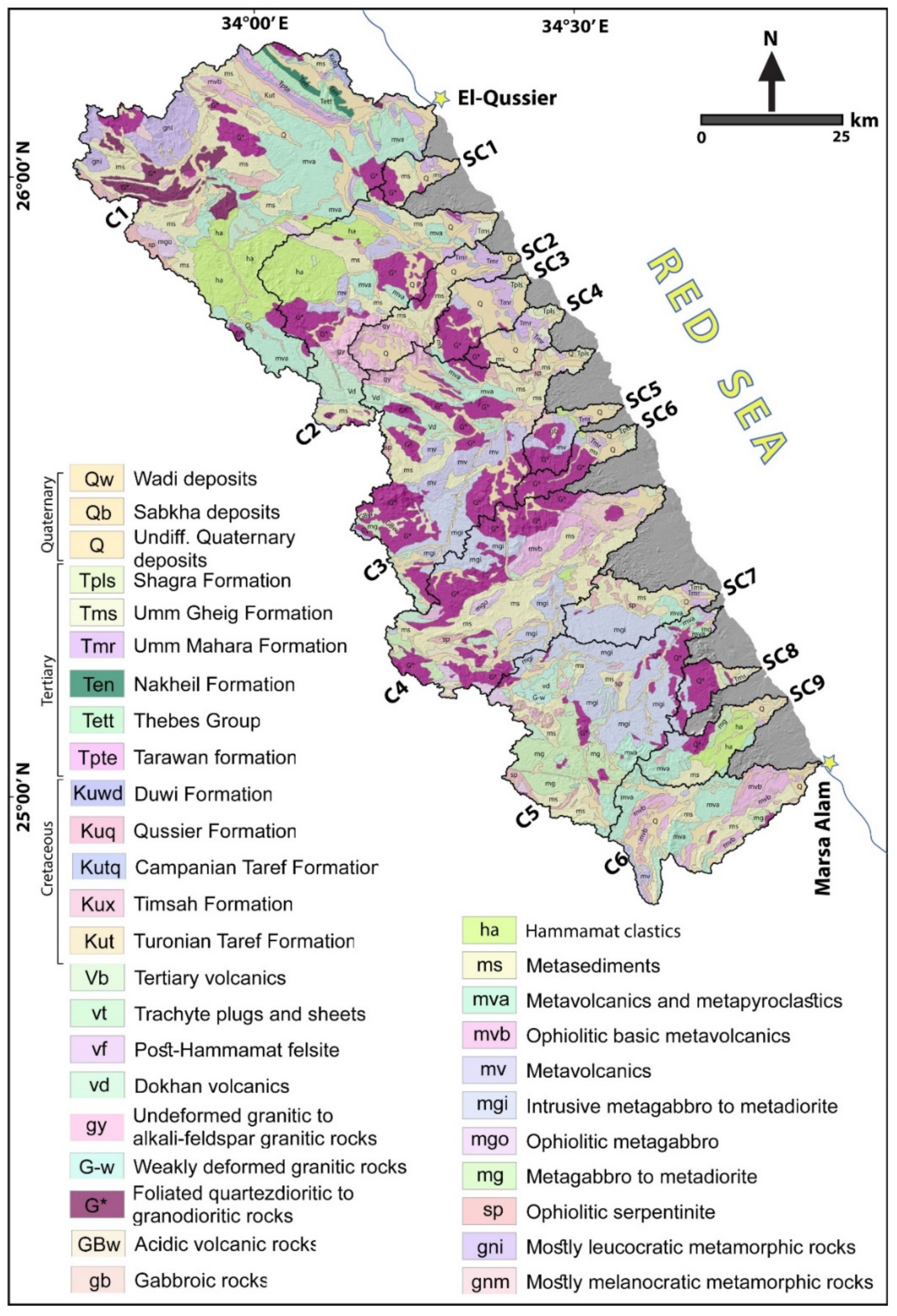
2.2. Geological Setting

Different geological units were identified from [26]. The basement units of the study area are mainly represented by medium-to high-grade metamorphic rocks, ophiolite serpentine including talc carbonate rocks, undifferentiated metagabbro to metadiorite, ophiolitic metagabbro, undifferentiated metavolcanics, ophiolitic metavolcanics, intermediate to acid metavolcanics and metapyroclastics, metamorphosed shelf sediments and volcanogenic rocks, molasse-type hammamat clastics, fresh olivine gabbro, deeply weathered grey granite (older granite), weakly deformed pink granitic (younger granite) rocks, unreformed granitic to alkali-feldspar granitic rocks, syenitic to alkali-feldspar syenitic rocks as a ring complex, alkaline andesitic to rhyolitic dokhan volcanics, post-hammamat felsite, and trachyte plugs and sheets, respectively [29] (Figure 2). The Upper Cretaceous period was recorded in the study area by Turonian Taref Formation, which is composed of fine- to medium-grained fluviatile and eolian sandstone, Coniacian-Santonian Timsah Formation, which includes shale, silt, and sandstone with two major oolitic iron-ore beds, Campanian Taref Formation, Campanian Qussier Formation, and Maastrichtian Duwi Formation [29] (Figure 2). The study area presents the Tertiary time through Tarwan Formation, Thebes Group, Nakheil Formation, Umm Mahara Formation, Umm Gheig Formation, and Shagra Formation, respectively [29] (Figure 2). The Quaternary rocks cover the study area by sabkha and wadi deposits [29] (Figure 2).

Regarding the general geomorphology of the Egyptian Eastern Desert, the studied zone is categorized into different linear zones [30]. The topographic maps and digital elevation model were preliminarily processed to examine the geomorphology of the study zone (Figure 4). The raster surface analysis tools in ArcGIS software, such as elevation, contour, slope, and aspect, aid in recognizing the different linear zones; the eastern coastal and inland strip zone, the high plateaus (mostly Miocene and Eocene), and the Pre-Cambrian Red Sea mountain hills (Figure 5a–d). Eastern desert of Egypt always reflects arid climatic conditions that vary from season to season and influence the hydrological characteristics of the drainage catchments in the study area. The temperatures range from 9.7 °C to 36.7 °C and reach 47 °C in the southern parts [21,31]. The humidity has been recorded as 43% in the summer seasons and 48% during winters [21,27].

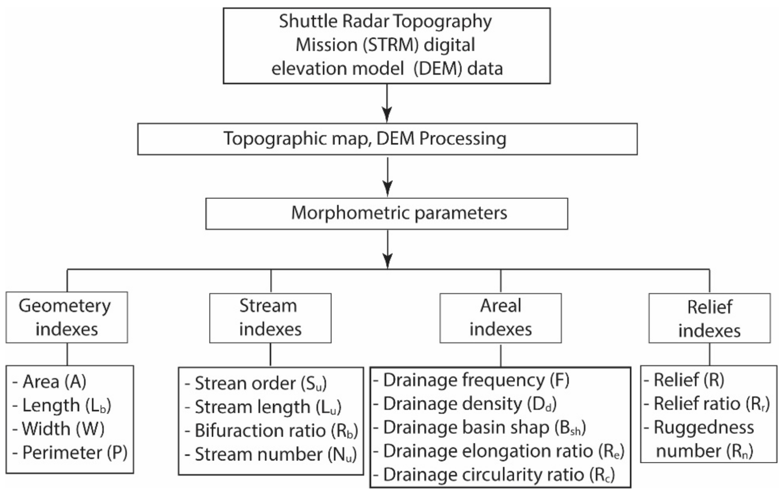
3. Data Collection and Methods

3.1. Morphometric Parameters

The raster and vector data (Shuttle Radar Topography Mission (SRTM) digital elevation model (DEM) data and geological maps) were collected and analyzed in order to investigate the morphometric features of the study catchments and sub-catchments (

Table 1. Available data that were processed in the study area.

Data	Sources	Date	Resolution
Shuttle Radar Topography Mission (STRM) digital elevation model data	https://earthexplorer.usgs.gov/	23 September 2014 00:00:00-05	30-m resolution
Geological maps of Egypt	EGPC and CONOCO, “Egyptian General Petroleum Corporation and CONOCO”, A geological map of Egypt	1987	1:500,000 scale

). ArcGIS 10.4 software package was run to process the different data and provide analysis, figures, and results of the study zone (Figure 4). The catchments drainage systems along the studied coastal line were generated from the (SRTM) digital elevation model data. The watershed boundaries, catchments sizes, and streams drainage networks were extracted using different algorithms in the ArcGIS spatial analysis tools (hydrology tools). The catchments were classified into 6 major catchments and 9 sub-catchments (Figure 5).

Quantitative morphometric analyses were applied on 15 catchments and sub-catchments to investigate the geomorphological properties of the drainage networks. The applied morphometric parameters were divided into four groups of calculations:

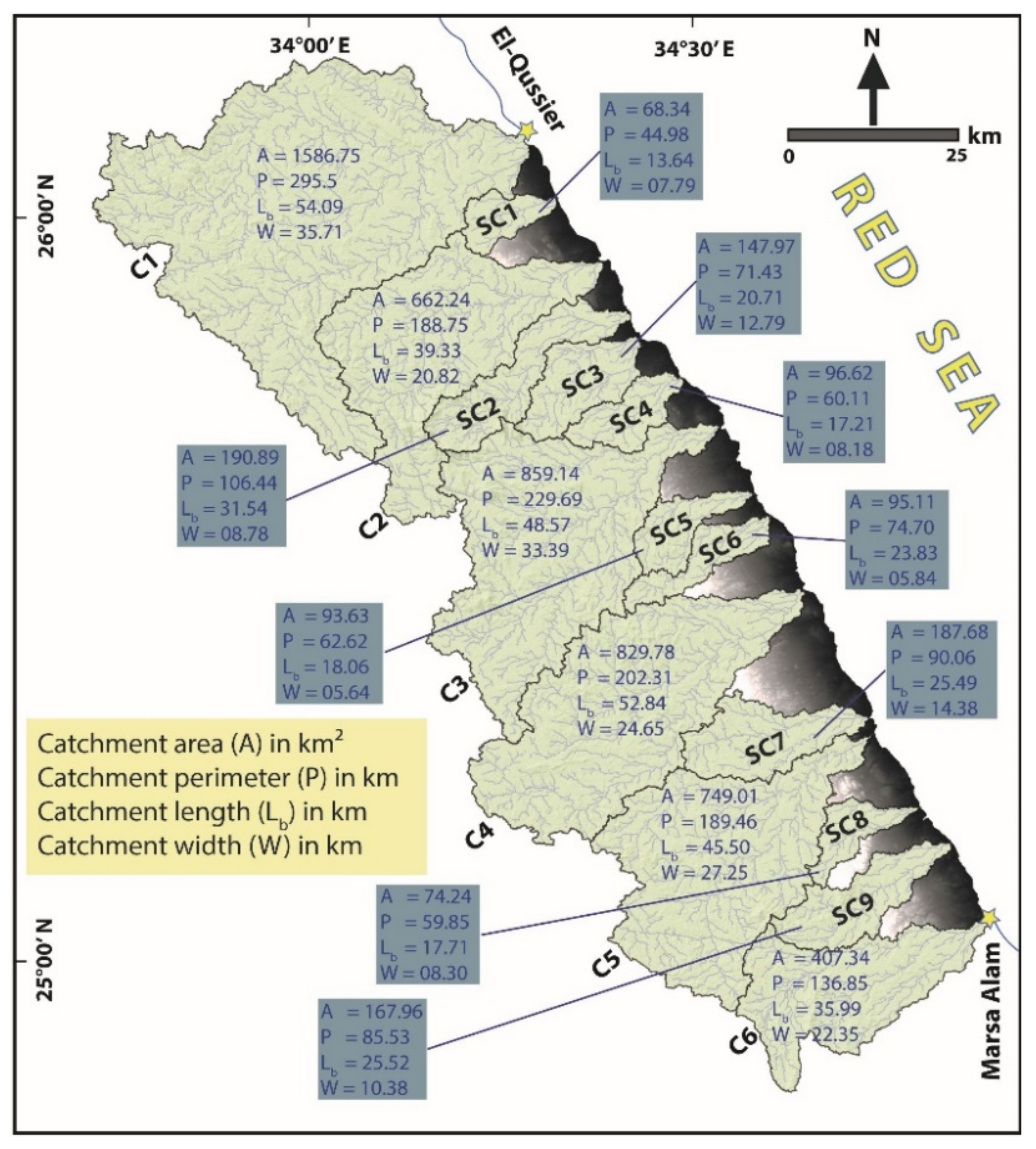
3.1.1. Catchment Geometry Indexes

Geometries were calculated based on four parameters, including catchment area index (A), catchment length index (L), catchment width index (W), and catchment perimeter (P) [17,19].

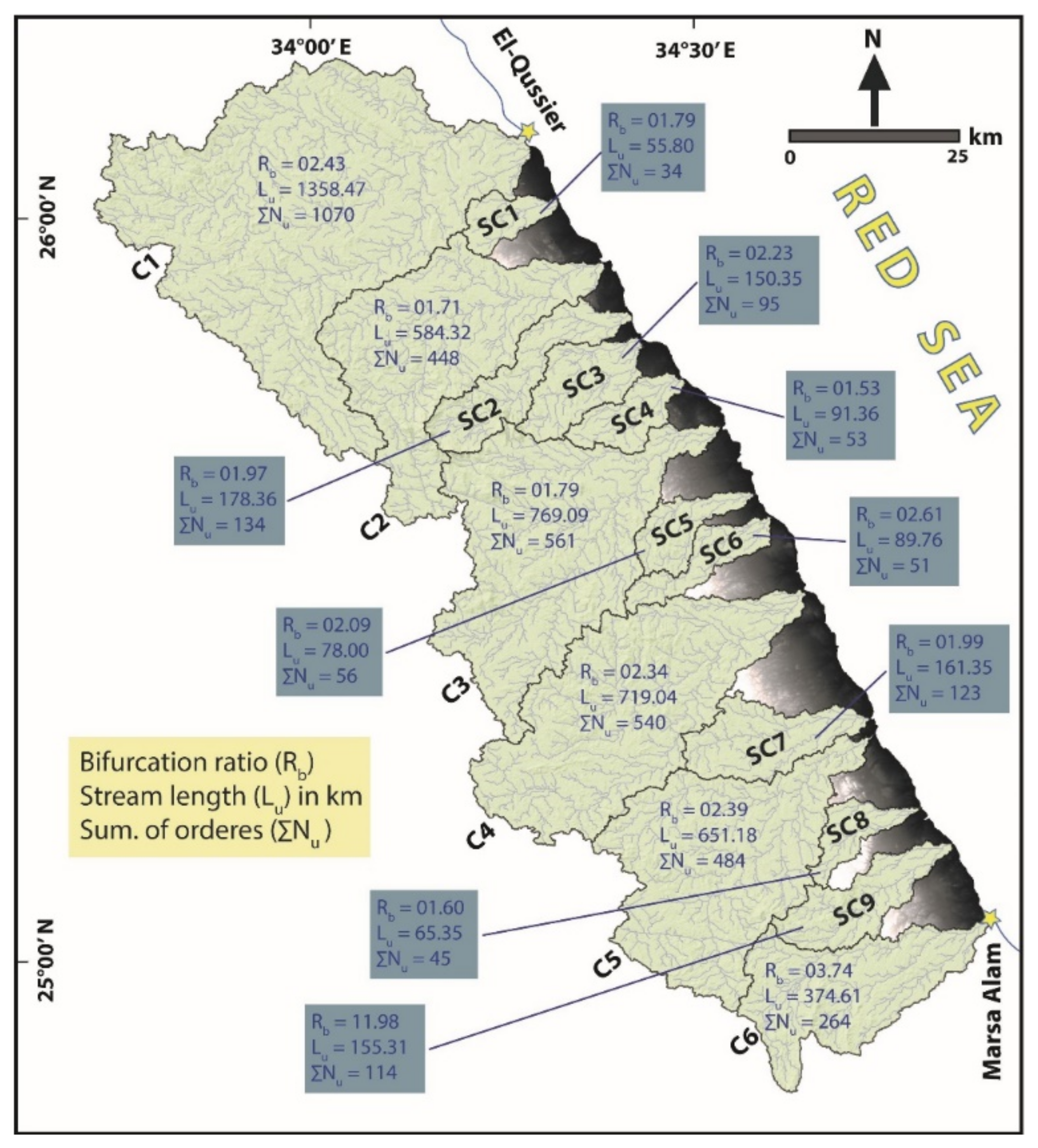
3.1.2. Stream Indexes

The stream characteristics are very helpful in order to complete the models for the basin analysis and watersheds behaviors. Stream indexes are completed by calculations of stream order (S_u), stream length (L_u), stream number, and bifurcation ratio (R_b) [20,31].

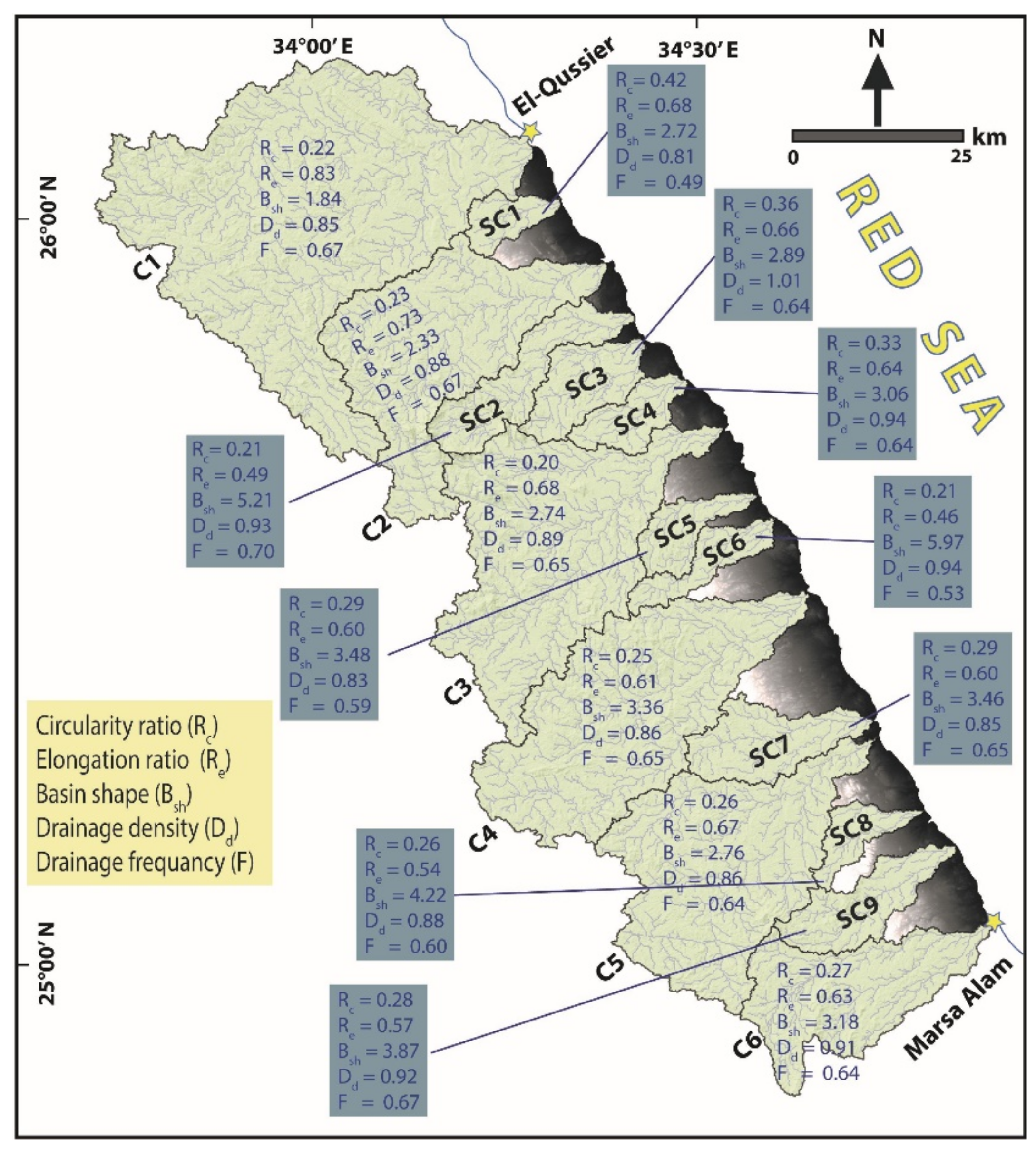
3.1.3. Areal Indexes

The areal aspects were estimated from different factors, including drainage frequency (F), drainage density (D_d), drainage basin shape (B_sh), drainage elongation ratio (R_e), and drainage circularity ratio (R_c) [32,33].

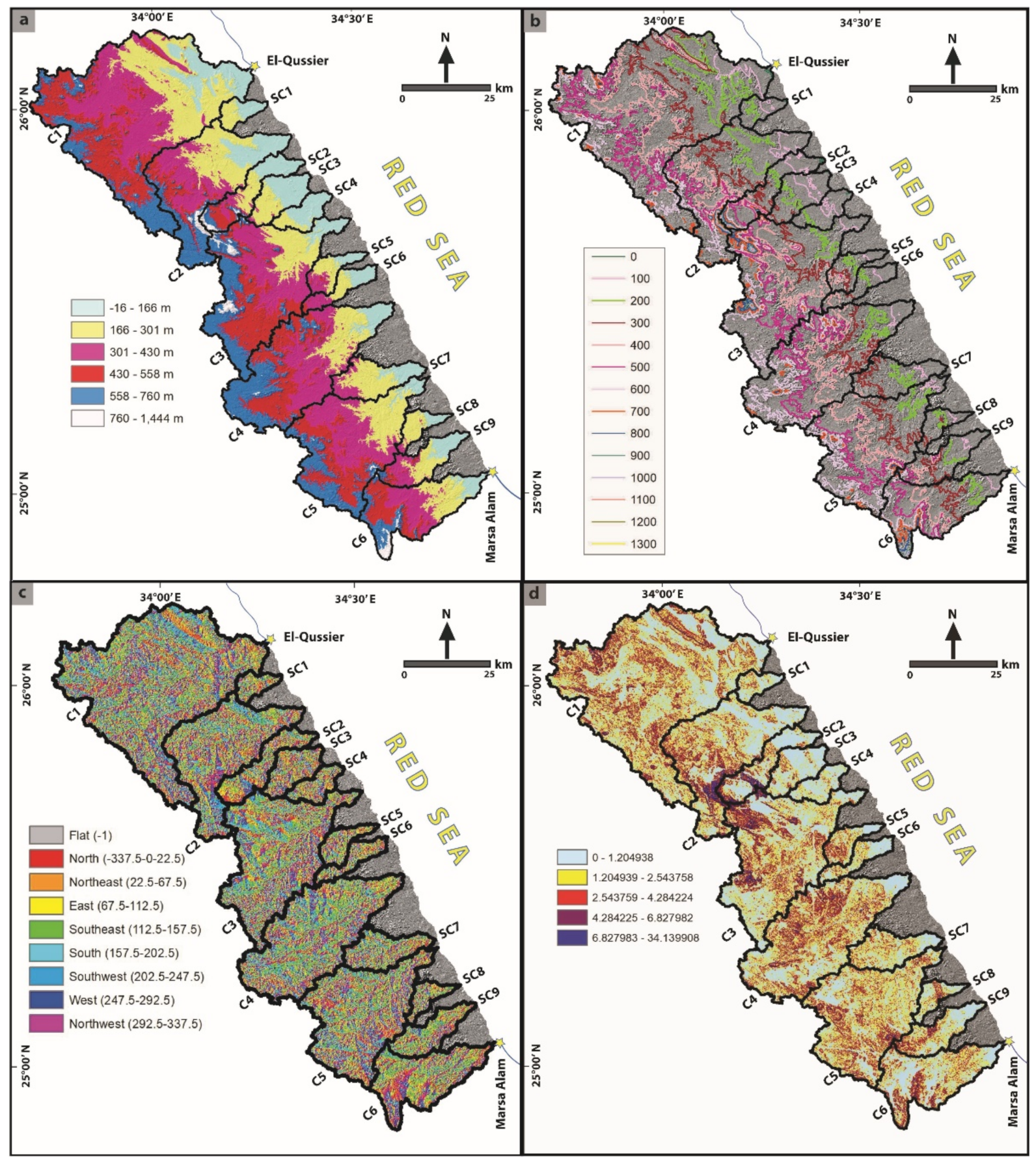
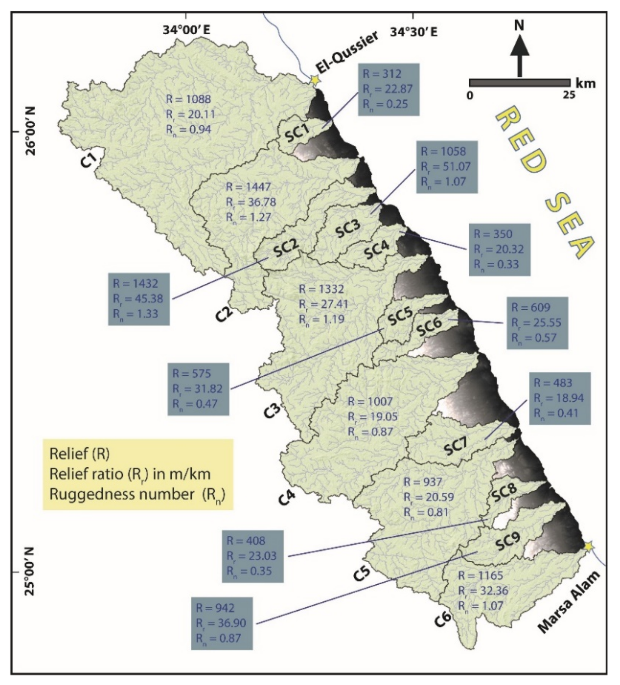
3.1.4. Catchment Relief Indexes

The relief indexes comprise catchment relief (R), catchment relief ratio (R_r), and catchment ruggedness number (R_n) [34,35,36].

All morphometric indexes were computed based on the equations suggested by [37,38]; the morphometric equations are illustrated in

Table 2. Computation methods of morphometric indexes, where, A = total area of a catchment, TSN = total stream numbers, TSL = total stream lengths, Z = highest point of a catchment, z = lowest point of a catchment, and D_d = drainage density.

Morphometric Indexes		Formula	References
Catchment geometry	Area index (A)	ArcHydro analysis	[34]
	Length index (Lb)	ArcHydro analysis	[34]
	Width index (W)	ArcHydro analysis	[34]
	Perimeter index (P)	ArcHydro analysis	[34]
Stream indexes	Stream order (Su)	Hierarchial rank	[21,36]
	Stream length (Lu) in km	Lu = L1 + L2 + …… Ln	[21,39]
	Bifurcation ratio (Rb)	Rb = Nu/Nu + 1	[21,34]
	Stream number (Nu)	Nu = N1 + N2 + …… Nn	[40]
Areal indexes	Drainage frequency (F)	TSN/A	[40]
	Drainage density (Dd)	TSL/A	[40]
	Drainage basin shape (Bsh)	Lb2/A	[16,40]
	Drainage elongation ratio (Re)	1.128 × A0.5/Lb	[34]
	Drainage circularity ratio (Rc)	4πA/P2	[41]
Relief indexes	Catchment relief (R)	H = Z − z	[41]
	Catchment relief ratio (Rr)	R/Lb	[34]
	Catchment ruggedness no. (Rn)	Dd × (R/1000)	[34]

.

3.2. SCS-CN Model

Soil Conservation Services and Curve Number (SCS–CN) method is a simple technique for rain-runoff modeling. The SCS–CN runoff equation was initiated in 1954 by the USDA SCS [35,42] and applied broadly in the Soil Conservation Service (SCS) in the hydrology section of the National Engineering Handbook (NEH-4) [43]. The CN is an empirical factor applied to hydrology for runoff prediction [36,44]. CN values are estimated based on the following three factors: land use, soil moisture characteristics, and soil type. Geological units were discriminated, and the soil types were recognized depending on the land use/cover of the study catchments and sub-catchments (Figure 2). The soil units are then categorized according to Hydrological Soil Groups (HSGs), indicating the infiltration ratios of the soil after rainfall storms. This method provides many assumptions. The first consideration states that the ratio of the exact quantity of direct runoff to the maximum runoff is equal to the ratio of the amount of infiltration to the potential maximum retention quantity. The second assumption confirms that the early abstraction quantity is a fraction of the maximum retention. The SCS number suggestion applies imperial methods to calculate the direct runoff quantity from study watersheds [36,42]. In regards to floods, the rainfall excess from the catchment outlets is described by a single value of CN and ranges from 0 to 100. In the present study, a rainfall–runoff model with a fixed grid size was initiated. An appropriate curve number value was calculated for each catchment area according to the standard SCS curve number tables [42], in addition to Antecedent Moisture Conditions (AMC). Different CN values for dry and wet conditions (AMC-I and AMC-III) were estimated from the following formulas:

CN1 = CN2/(2.281 − 0.01281 CN2)

CN3 = CN2/(0.427 − 0.00573 CN2)

and the recharge capacity values (S) were calculated by subtracting the value of the weighted CN as follows:

S = (25400/CN2) − 254

precipitation data (P) that registered between 2005 and 2020 were used to calculate the direct runoff (Q) from the following equation:

Q = (P − 0.3 S)²/(P + 0.7 S)

where, Q is the runoff depth in mm, P is the rainfall in mm, S is the potential retention, and Ia is the initial abstraction ratio (Ia = 0.2 S).

CN = sum (CNi × Ai)/sum Ai

where, CN is the area-weighted curve number for the catchment, CNi is the curve number for land use-soil group catchment, Ai is the total area of land use-soil group catchment, and n is the number of land use-soil polygons for each drainage catchment.

3.3. Watershed Modeling System (WMS)

The goal of this section is to establish a hydraulic and hydrologic model, delineate catchments, and extract hydrographical curves by using advanced software such as WMS and HEC-HMS. For this purpose, different datasets were collected and categorized, including digital elevation models (DEMs), storm data, and soil type. WMS is an effective watershed computer simulation and modeling software package that is used to develop the watershed hydrologic and hydraulic modeling. WMS software (version 11.1) develops different hydrological models and provides tools to automate digital terrain models such as catchments delineations and hydrographic curves. The hydrology tools inside the WMS program can easily run many models, including the interaction between the surface-water and groundwater, wetland areas, different kinds of sediments, pollution simulation, leakage and storms analysis, and submerged surface [41]. This software also provides a control mechanism that is able to evaluate the input data and check if there are any modeling errors [20,36]. In addition, HEC-HMS version 4.8 is an another program that automates and simulates the different hydrological properties of hydrographic catchments and sub-catchments. The HEC-HMS software processes the collected data in order to automate catchments and sub-catchments boundaries, extract catchments drainage systems, and compute the hydrographic curves for the different watersheds.

3.4. Flash Flood Hazards Assessment Parameters

In this work, the Hydrologic Modeling System (HEC-HMS) was adapted to provide a hydrological simulation in order to complete the hydrologic characteristics of the catchments and sub-catchments. Following recent hydrological models [36], the loss estimation techniques, in addition to the lag-time estimation method, are the most used methods to extract the hydrological parameters for the rainfall–runoff relationship.

Many factors were calculated to estimate and evaluate the flood risks, including lag time (T_Lag), time of concentration (T_c), flow velocity (V), peak discharge value (Qp), and flood volume value (Qt).

Main flash flood parameters were calculated based on the formula stated by [45,46], and they are listed in

Table 3. Computation methods of main flash floods parameters.

Equation	Abbreviation Description
TLag = L0.8(S + Ia)0.7/1900√Y	TLag: lag time (h); Y: basin slope (%); Tc: time of concentration (min); V: flow velocity; La: catchment length; Qp: peak discharge (m3/s); A: catchment area (Km2); Tp: time to peak (h); Δt: duration of designed storm; Q: direct runoff (mm); p: rainfall return periods (cm); S: potential maximum retention (mm); Ia: amount of total water before of flood; CN: curve number
Tc = 0.0001(L0.77/S0.385)
V = 0.2279La/TC
Qp = 0.208A/Tp
Tp = Δt/2 + TLag
Q = (p − 0.2S)2/(p + 0.8S)
Q = (p − Ia)2/(p − Ia + S)
Ia = 0.2S
S = 1000 − 10CN/CN S = 25,400 − 254CN/CN

.

4. Results

4.1. Quantitative Morphometric Analysis

The largest area of the 15 studied catchments and sub-catchments was measured for catchment no. 1 (C1 = 1586.75 km²), while sub-catchment no. 1 was estimated as the smallest sub-catchment in the study area (SC1 = 68.34 km²) (

Table 4. Catchments geometry calculations of the study catchments and sub-catchments.

Catchments/ Sub-Catchments	Area (km2)	Perimeter (km)	Length (km)	Width (km)
C1	1586.75	295.55	54.09	35.71
C2	662.24	188.75	39.33	20.82
C3	859.14	229.69	48.57	33.39
C4	829.78	202.31	52.84	24.65
C5	749.01	189.46	45.50	27.25
C6	407.34	136.85	35.99	22.35
SC1	68.34	44.98	13.64	07.79
SC2	190.89	106.44	31.54	08.78
SC3	147.97	71.43	20.71	12.79
SC4	96.62	60.11	17.21	08.18
SC5	93.63	62.62	18.06	05.64
SC6	95.11	74.70	23.83	05.84
SC7	187.68	90.06	25.49	14.38
SC8	74.24	59.85	17.71	08.30
SC9	167.96	85.53	25.52	10.38

; Figure 6). Based on [37], 10 catchments and sub-catchments were recognized as large catchments (greater than 100 km²), while five were considered as small catchments (SC1, SC4, SC5, SC6, and SC8 are less than 100 km²) (Table 4; Figure 6). Similarly, the largest catchment perimeter was recorded for C1, with a size of 295.55 km, and the smallest value was calculated for SC1, with a size of 44.98 km (Table 4; Figure 6). The measured lengths of the study zone ranged from 13.64 km (SC1) to 54.09 (C1). The largest catchment width was measured for C1 (35.71 km), while the smallest one was recorded for SC5 (5.64 km).

Stream orders of the study catchments and sub-catchments vary from third-orders to sixth-orders. The dominant orders are the fifth and third-orders that were recognized for (C2:C6) and (Sc1, Sc4, Sc5, Sc6, and Sc8), respectively. The calculated orders are classified as follows: third-orders cover an area of about 6.81% of the entire studies zone, fourth-orders control around 11.17% of the catchments and sub-catchments, fifth-orders cover around 56.42% of the study zone, and finally, sixth-orders occupy an area of about 25.52% of the proposed zone. The total stream length of the study area reaches 5482.40 km. The stream lengths of the catchments and sub-catchments range from 55.80 km (SC1) to 1358.47 km (C1) (

Table 5. Catchments characteristics of stream, areal, and relief indexes of the study catchments and sub-catchments.

Catchments/Sub-Catchments	Stream Indexes			Areal Indexes					Relief Indexes
	Rb	Lu (m)	ΣNu	Rc	Re	Bsh	Dd	F	R (m)	Rr (m/km)	Rn
C1	2.43	1358.47	1070	0.22	0.83	1.84	0.856	0.674	1088	20.11	0.94
C2	1.71	584.32	448	0.23	0.73	2.33	0.882	0.671	1447	36.78	1.27
C3	1.79	769.09	561	0.20	0.68	2.74	0.895	0.653	1332	27.41	1.19
C4	2.34	719.04	540	0.25	0.61	3.36	0.866	0.650	1007	19.05	0.87
C5	2.39	651.18	484	0.26	0.67	2.76	0.869	0.647	937	20.59	0.81
C6	3.74	374.61	264	0.27	0.63	3.18	0.919	0.642	1165	32.36	1.07
SC1	1.79	55.80	34	0.42	0.68	2.72	0.816	0.491	312	22.87	0.25
SC2	1.97	178.36	134	0.21	0.49	5.21	0.934	0.702	1432	45.38	1.33
SC3	2.23	150.35	95	0.36	0.66	2.89	1.016	0.642	1058	51.07	1.07
SC4	1.53	91.36	53	0.33	0.64	3.06	0.945	0.543	350	20.32	0.33
SC5	2.09	78	56	0.29	0.60	3.48	0.833	0.592	575	31.82	0.47
SC6	2.61	89.76	51	0.21	0.46	5.97	0.943	0.532	609	25.55	0.57
SC7	1.99	161.35	123	0.29	0.60	3.46	0.859	0.659	483	18.94	0.41
SC8	1.60	65.35	45	0.26	0.54	4.22	0.880	0.602	408	23.03	0.35
SC9	1.98	155.31	114	0.28	0.57	3.87	0.924	0.677	942	36.90	0.87

; Figure 7). The highest R_b value is recorded for SC6 as 3.74, and the lowest value was estimated as 1.53 for SC4 (Table 5; Figure 7).

The calculated stream frequency (F) of the entire studied zone is 9.41. The lowest value was recorded for SC1 at 0.497, while the highest value was recognized for SC2 at 0.701 (Figure 8). The drainage density values of the study catchments and sub-catchments ranges from 0.856 km/km² (C1) to 1.016 km/km² (SC3) (Table 5; Figure 8). The basin shape index indicates the lowest reading for C1 with a value of 1.84 and the highest value for SC6 at 5.97 (Table 5; Figure 8). The calculated values of the catchment elongation ratio (Re) range between 0.46 for SC6 and 0.83 for C1 (highest value) (Table 5; Figure 8). The catchment circularity ratio (R_e) recorded its lowest value at 0.20 for C3, while the highest ratio was estimated for SC1 (0.42) (Table 5; Figure 8).

The catchment relief indexes of the entire catchments and sub-catchments are given in Table 5 and illustrated in Figure 9. The basin relief values vary from 312 m (SC1) to 1447 m (C2). The relief ratio index provides 19.05 m/km for C4 as the lowest value and 51.07 m/km for SC3. SC4 and SC2 provide the lowest and highest values (0.25 and 1.33), respectively.

4.2. Curve Number (CN)

The results of the curve numbers were computed according to the classification of hydrologic soil and the total catchments area. The curve number values range from 80.66 for C3 to 85.20 for C6 (

Table 6. Flash floods characteristics of the study area during October 2009 and 2019 storm events.

Main Catchments	Catchments Hydrological Data				2009 Storm Event		2019 Storm Event
	CN	TLag (h)	V (m/s)	Tc (h)	Qp (m3/S)	Qt (m3)	Qp (m3/S)	Qt (m3)
C1	83.75	2.42	26.59	7.724	70	733,184.00	51	512,000.00
C2	82.36	2.19	26.71	5.592	36	250,048.00	19	167,936.00
C3	80.66	2.38	27.39	6.736	77	618,496.00	42	81,920.00
C4	82.50	2.46	28.92	6.939	113	831,488.00	63	491,520.00
C5	84.30	2.08	26.27	6.578	46	368,640.00	26	221,184.00
C6	85.20	1.89	29.89	4.573	57	507,904.00	30	319,488.00
SUM.						3,309,760.00		1,794,048.00

).

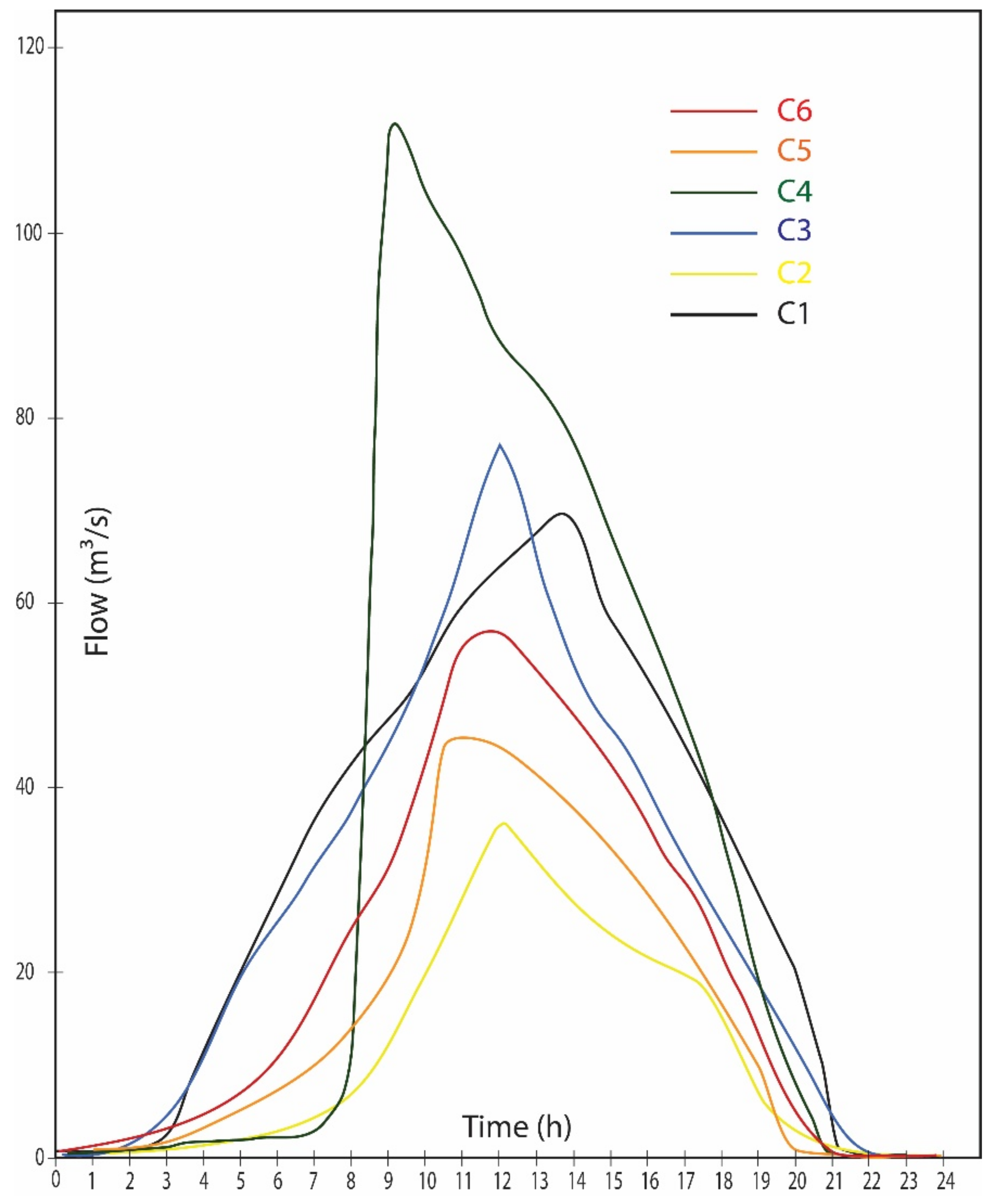
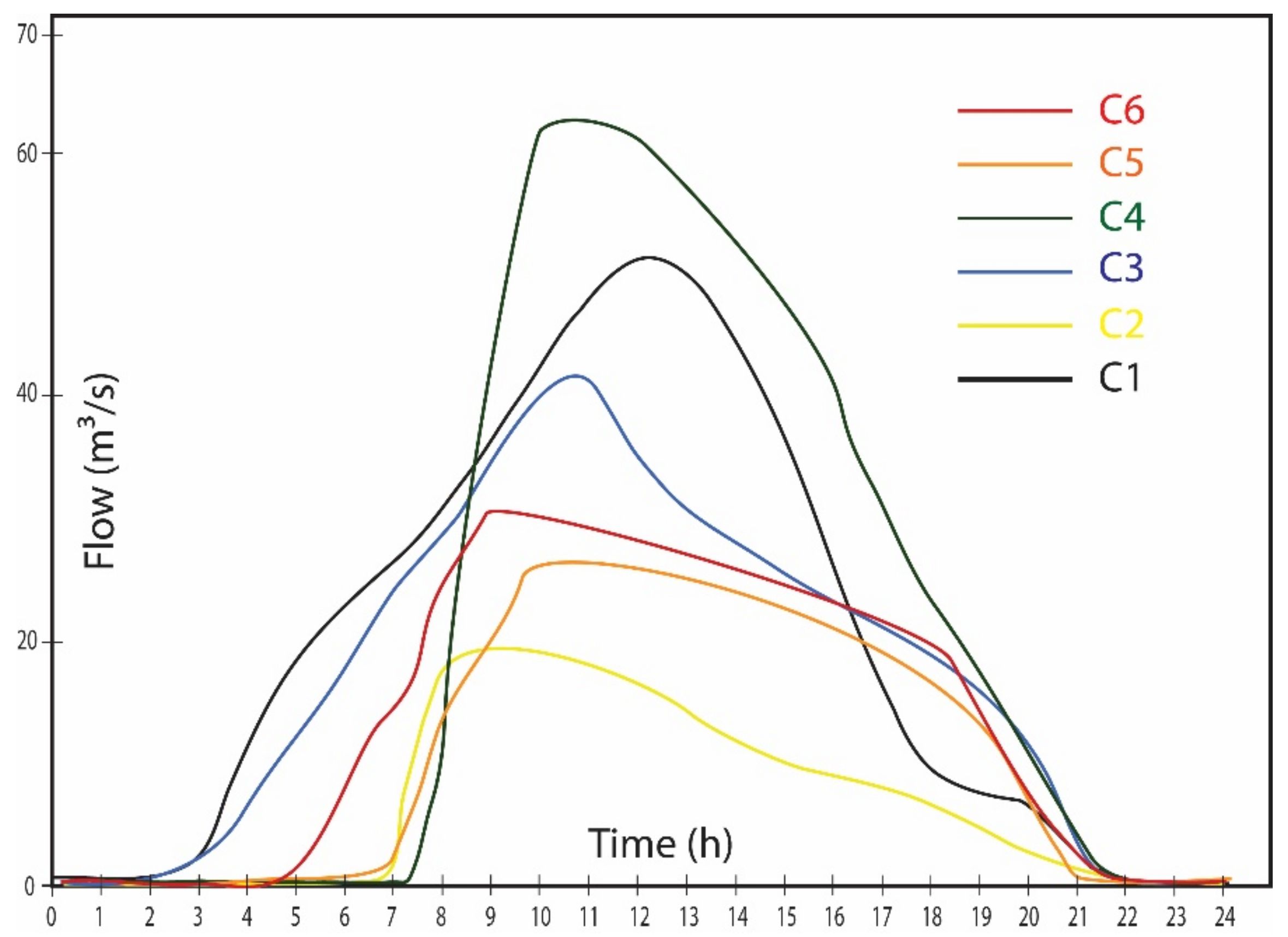
4.3. Watershed Modeling System (WMS)

Six hydrographs were simulated and modeled for the major catchments (C1:C6) using the Hydrological Modeling System (HEC-HMS) (Figure 10 and Figure 11). The software was run for many hydrological models such as hydrologic routing, unit hydrograph, and event infiltration [36].

4.4. Flood Risk Assessment

In this work, rainfall–runoff relationship was modeled from lag-time calculation and loss estimation methods. Many data such as DEMs, soil data, loss rate, base flow, and time concentration were combined to intiate the suitable hydrological models. The extracted runoff hydrographic curves for storms 2009 and 2019 are illustrated in Figure 10 and Figure 11, and their hydrological results are tabled in Table 5 and Table 6. In this study, the minimum value of the lag time was recorded for C6 (1.89 h), while its maximum value was calculated for C5 (2.46 h). The calculated concentration times were recorded as a lowest time for C6 (4.573) and a highest time for C1 (7.724). The water velocities of the study catchments are recording the lowest velocity for C5 (26.27 m/s) and the highest velocity for C6 (29.89 m/s). The peak discharge values (Qp) were calculated for the major six catchments and provide 117 m³/s and 70 m³/s for the storms of October 2009 and 2019, respectively. The peak discharge values of October 2009 were estimated to range from 36 (C2) to 113 (C4), while Qp values of the next studied storm event were recorded to range from 19 (C2) to 63 (C4). Finally, the flood volumes were estimated for the major catchments and provided 3,309,760.00 m³ and 1,794,048.00 m³ for October 2009 and 2019 storms, respectively. In October 2009, flood volume values recorded 250,048.00 m³ and 831,488.00 m³ for C2 and C4, respectively. 81,920.00 m³ and 512,000.00 m³ flood volume values were estimated during October 2019 storm for C3 and C1, respectively.

5. Discussion

Flash flooding represents one of the quickest and huge destructive natural hazards, particularly in arid regions. It is a result from extensive climate changes that cause very strong storm events and huge amounts of rainfall. Monitoring and analyzing these storms provide very important keys to minimizing their negative effects and report a precious future prediction. Numerous storm events were investigated using various techniques in order to gain insights into the main morphometric and hydrologic characteristics of the storm regions [2,8,47,48,49,50,51,52]. Many parameters can affect the potential of the storms, including soil types, the geological and morphological setting, climatic conditions, and human activities. Many factors are responsible for exaggerating the negative impacts of flood risks. The scarcity of monitoring stations and absence of the early warning networks are the biggest weakness in planning flood hazards management. The Egyptian Red Sea coast is usually exposed to many extensive natural hazards that harm the sustainability plans of country development. Recent studies have used modern techniques such as remote sensing and GIS to model flash floods potential in order to help decision-makers adjusting suitable strategies against the negative impacts of this particular natural risks [36,53].

The present study investigates in details the flash floods risk assessment of one of the important Red Sea coastal zones. Discussing the morphometric analysis and hydrological characteristics of the catchments and sub-catchments between El-Qussier and Marsa Allam during October 2009 and 2019 storm events is the key for evaluating the flood risk levels and understanding the common behaviors of the similar storm events.

The hydrological characteristics and related flash flood risks have been discussed in many different methods for several regions. The geomorphological hazards, including flash floods along the Egyptian Red Sea coast between Safaga and Quseir, were assessed by the study of [26]. The authors integrated geomorphological, geological, remote sensing, and climate data to confirm the paper results. The conclusion of the authors in Ref. [26] stated that the entire coastal line between Safaga and Quseir has been hit by floods frequently and these risks will accelerate based on different conditions. A study in [26] recommended proposing some dams to mitigate the effect of the flood risks. In [8] authors estimated the flash flood hazard along the Saint Katherine road in Sinai using morphometric analysis and remote sensing data. Morphometric analysis in [5] initiated a model that classified the catchments of the study area into high and low risks. While they recommended establishing a number of dams on the main channels, they believed that these dams might not stop the total flood water. A study in [21] processed seismicity and remote sensing data to compute the morphometric indexes in order to assess the geo-natural hazards of the region between Marsa-Alam and Abu Ghuson coastal line of the Egyptian Red Sea coast. In order to minimize the effect of flood risks and protect the urban regions, authors in ref. [21] recommended some strategies, including establishing dams in critical locations, particularly in wadis, and establishing any new projects away from the flooding courses.

Quantitative morphometric analyses of the 15 catchments and sub-catchments were calculated to define the properties of the drainage systems of the study zone. Discussing the morphometric parameters of the study area is very valuable to understand the tectonic and geomorphic signatures of the different landforms [32,37,40]. The geometry indexes were calculated along the Red Sea coast to examine the natural hazard signals [21]. In the present study, the geometry indexes were extracted to aid in explaining the classification of the catchments and sub-catchments. Linear indexes that refer to the properties of the drainage network were used widely to evaluate the flood hazards in many regions [40,54,55]. Ref. [36] calculated the linear indexes to assess the flood hazards in southwest Sinai in Egypt. In our study, several linear indexes were extracted, including stream orders, total stream lengths, and the bifurcation ratio. Particularly, stream numbers and order are very effective indexes in hydrological studies. The majority of stream orders were recorded for the fourth-orders in five catchments. The high leveling of branching in our drainage system indicates high possibilities of water flows. The results of the Bifurcation ratio index (R_b) indicate that all of the investigated catchments reflect low values (1.53–3.74), and their frequencies (F) produce values between 0.491 (SC1) and 0.702 (SC2) and this tends to give suitable conditions for flash flood possibilities.

Morphometric drainage density (D_d) reveals important catchment characteristics, including land infiltration capacity, climatic conditions, and vegetation cover [56,57]. Author in ref. [39] stated that the average drainage density index is 0.93 km/km², which reaches 1.24 km/km² in mountain areas that have high rates of precipitation. Catchments of high drainage density show high rate of flood flows with low amount of groundwater storage, while the low drainage density values indicate suitable conditions for infiltration rate and decreasing rate of runoff potential in addition to erosion-resistant fractured hard rock of the investigated zone [36,58]. The drainage densities of the study zone reflect low relief, dense vegetation, and a low amount of groundwater for the majority of the study catchments and sub-catchments. The D_d index results indicated that, the contribution of local rains to the groundwater is low as expected. Consequently, high values of stream frequency (>0.5) provide high possibilities for water runoff collection that reflect impermeable sub-surface beds, high relief, and minimum infiltration rates [8,36,59]. Regarding the density values of the study catchments and sub-catchments, the calculations give moderate values between 0.816 (SC1) and 0.945 (SC4). The only high drainage density refers to SC3 with 1.016 and this value can be considered as a D_d anomaly. The previous results reflect moderate relief, moderate level of impermeable subsurface beds, and moderate conditions for groundwater, particularly in the basement rocks area. According to the general morphology of the study zone, the safest zone against the flash flooding risk is the inland coastal zone. This is because of the high infiltration covering and the gentle slope plain strip [49,53]. In contrast, the impervious basement rocks of the western Red Sea mountain hills reflect high conditions of runoff possibilities [36].

The relief of landforms depends mainly on the topographic and tectonic developments [21,40]. In the current study, several topographic maps illustrated the topographic evolution of the study area (Figure 5). Refs. [21,60] categorized landscape slopes into nine groups: from flat running to very steep zones. In this study, the gradient slopes of the study catchments and sub-catchments give the steepest values for the western linear zone. Elevation, contouring, and aspect maps illustrated the topographic signals of the study zone. Relief indexes including relief, relief ratio, and ruggedness number, are important factors that aid in understanding the structural complexity of the topography of any region [21].

The curve number (CN) is a simple example of a moderate flood evaluation factor. It is applied in flood management projects and engineering designs. Low CN curve values dominantly cover the catchments that have beds with a high degree of infiltration losses. On the other hand, catchments with high CN values are mainly composed of hard rocks and dominantly characterized by a large amount of runoff flow and a small amount of infiltration abstraction [61]. According to the SCS classification, major catchments (C1:C6) provide high CN values as 83.75, 82.36, 80.66, 82.50, 84.30, and 85.20, respectively (Table 6). CN results indicate that the majority of the study zone is expected to give high peak discharges. Because of the estimated large areas, the highest peak discharge is expected to be recorded for C1 (Table 6), but abnormally the highest values were recorded for C3 and C4 in 2009 storm and C4 during storm of 2019. Accordingly, this is the second recorded anomaly in the morphometric and hydrological calculations.

The relief and slope indexes are very effective parameters for evaluating the intensity of flash flooding hazards, particularly in arid regions. Generally, steeper catchments provide suitable conditions for runoff water to be faster, more destructive, and produce higher catchment discharges. In the study area, the western strip is the highest subjected zone to flash floods because of the combining impervious soils and very steep slopes [36,53]. The steep slope lands are characterized by high reliefs and relief ratios, in addition to low flow concentration time. During such strong storms, ref. [62] confirmed that the lower concentration flow time leads to more hazardous runoff. The relief of the major catchments ranges from 937 m (C5) to 1447 m (C2), while the concentration-time (T_c) of the six catchments water flows give the lowest times for C6 and C2 (4.573 h and 5.592 h, respectively) and the highest time was recorded for C1 (7.72 h). Accordingly, C2 represents the most hazardous catchment with high relief and relief ratio values with low concentration-time (Table 5 and Table 6). Total flood volumes are estimated based on the catchment area, catchments total stream length, and maximum peak discharges.

Researchers in [36] applied geospatial analysis and a hydrograph model (HEC-HMS) in the WMS software to initiate flow hydrographs of flash floods in the Wadi Al Aawag drainage catchments in south Sinai. In addition, they used SCS unit approach to estimate the surface water and peak flow. They performed correlation analysis between many flood parameters that stated that, flood volume and peak discharge give positive consistency with the basin area, basin stream length, runoff depth, fellow velocity, and curve number. Authors in ref. [28] recommended constructing alternative barriers at some upstream parts to minimize flood risks, proposing storage dams, and initiating monitoring and warning systems. Authors in ref. [20] used Storm Water Management Model (SWMM) and WMS to initiate hydraulic and hydrologic model of the Aymmama River watershed in Istanbul. They concluded that integration of ArcGIS and WMS softwere is very effective in establishing hydraulic and hydrologic effective models and flash flood simulations.

The hydrological characteristics of the major catchments stated that C4 has the maximum runoff volumes and the peak discharge during October 2009 storm event, while October 2019 storm provided the maximum peak discharge for C4 and maximum runoff volumes for C1 as an anomalous record (Table 6; Figure 10 and Figure 11). CN and runoff velocity indexes of the major catchments provided relatively similar values, which lead us to consider these two values as minor effective values of the examined storm events (Table 6). The maximum area, longest stream length, and the highest total of stream numbers are recorded for C1 as 1586.75 km², 1358.47 m, and 1070, respectively (Table 4 and Table 5).

From the above discussion, integration between remote sensing technique, geospatial analysis, morphometric analysis, and hydrological modeling has proven that these methods are very effective for examining and assessing the different geological hazards [9,10,28,56]. This study focuses on examining the hydrological and morphometrical properties along a very important coastal line zone to fill the geo-hazard studies gap between [11,28]. While results from this study are consistent with the results that come from [11,28]. In contrast, results from [26] show inconsistencies with this study. This inconsistency comes from mapping some low-risk catchments in [26], while analysis of this paper reflects high preliminary signals for all catchments and sub-catchments.

Some researchers, such as [11,42,47], suggested and recommend some effective techniques to prevent or at least break down flood risk negative impacts. The suggested solutions recommended dams and bridge constructions, in addition to investigating and evaluating both recorded and predicted flash floods.

6. Conclusions and Recommendations

This work is focusing on assessing flash flood hazards in the strip zone between El-Qussier and Marsa-Alam along the eastern Egyptian Red Sea coastal line by investigating and calculating the morphometric analysis and hydrological characteristics of the catchments and sub-catchments of the study zone during October 2009 and 2019 storm events. In this study, the lack of geological hazards information was compensated in order to fill the study gap in a very important coastal zone of the Egyptian Red Sea coast. Morphologically, the studied zone are classified into three strip zones and the most hazardous signals are distributed along the western strip. General quantitative morphometric results indicate that, all catchments and sub-catchments provide low R_b values, and their total frequencies ranged from 0.497 (SC1) to 0.701 (SC2). SC1 and SC2 are located in the northern part of the study zone. R_b and F indexes provide suitable conditions for flash flood events. The investigated catchments and sub-catchments have nearly moderate densities. The only high-density value is 1.016 (SC3), which is remarked as an anomaly index factor. The density index values reflect moderate relief, semi-permeable subsurface beds, and semi-dense vegetation cover, particularly along the western strip zone (Pre-Cambrian Red Sea mountainous zone). The hydrological characteristics of the major catchments (C1:C6) indicate dominant moderate conditions for flash floods. This adds many explanations to our understanding of the behaviors of the hydrological models and underground water storage.

According to the general results of this study, many strategies have been recommended to minimize the negative effects of the major storms on infrastructure and population sites. These strategies include:

• Studying in details the seismic/tectonic behaviors of the future strategic projects and huge constructions.
• Constructing dams in the most hazardous spots along the specific valleys.
• Initiating channels and valleys mouths to receive the great rainfall accumulation toward the Red Sea.
• Planning the future major projects and constructions to be away from the courses of the major floods.
• Establishing hazard monitoring stations along the risky regions.

References

1. IFRC. World Disasters Report 2020: Come Heat or High Water; IFRC: Paris, France, 2020. [Google Scholar]
2. Boruff, B.J. Environmental Hazards: Assessing Risk and Reducing Disasters, 5th; Smith, K., David, N., Eds.; Routledge: London, UK, 2009; Volume 47, pp. 454–455. [Google Scholar] [CrossRef]
3. Dankers, R.; Feyen, L. Flood Hazard in Europe in an Ensemble of Regional Climate Scenarios. J. Geophys. Res. Atmos. 2009, 114, 1–16. [Google Scholar] [CrossRef]
4. Velasco, M.; Versini, P.A.; Cabello, A.; Barrera-Escoda, A. Assessment of Flash Floods Taking into Account Climate Change Scenarios in the Llobregat River Basin. Nat. Hazards Earth Syst. Sci. 2013, 13, 3145–3156. [Google Scholar] [CrossRef] [Green Version]
5. Wu, S.H.; Pan, T.; He, S.F. Climate Change Risk Research: A Case Study on Flood Disaster Risk in China. Adv. Clim. Chang. Res. 2012, 3, 92–98. [Google Scholar] [CrossRef]
6. Davis, R. World Disaster Report—Most Deaths Caused by Food. 2014. Available online: https://floodlist.com/dealing-with-floods/world-disasters-report-100-million-affected-2013 (accessed on 6 October 2016).
7. Prama, M.; Omran, A.; Schröder, D.; Abouelmagd, A. Vulnerability Assessment of Flash Floods in Wadi Dahab Basin, Egypt. Environ. Earth Sci. 2020, 79, 114. [Google Scholar] [CrossRef] [Green Version]
8. Youssef, A.M.; Pradhan, B.; Hassan, A.M. Flash Flood Risk Estimation along the St. Katherine Road, Southern Sinai, Egypt Using GIS Based Morphometry and Satellite Imagery. Environ. Earth Sci 2011, 62, 611–623. [Google Scholar] [CrossRef]
9. Bathrellos, G.D.; Karymbalis, E.; Skilodimou, H.D.; Gaki-Papanastassiou, K.; Baltas, E.A. Urban Flood Hazard Assessment in the Basin of Athens Metropolitan City, Greece. Environ. Earth Sci. 2016, 75, 319. [Google Scholar] [CrossRef]
10. Petrucci, O.; Aceto, L.; Bianchi, C.; Bigot, V.; Br, R.; Pereira, S.; Kahraman, A.; Kılıç, Ö.; Kotroni, V.; Llasat, M.C.; et al. Flood Fatalities in Europe, 1980–2018: Variability, Features, and Lessons to Learn. Water 2019, 11, 1682. [Google Scholar] [CrossRef] [Green Version]
11. Moawad, M.B. Analysis of the Flash Flood Occurred on 18 January 2010 in Wadi El Arish, Egypt (a Case Study). Geomat. Nat. Hazards Risk 2013, 4, 254–274. [Google Scholar] [CrossRef] [Green Version]
12. Youssef, A.M.; Sefry, S.A.; Pradhan, B.; Alfadail, E.A. Analysis on Causes of Flash Flood in Jeddah City (Kingdom of Saudi Arabia) of 2009 and 2011 Using Multi-Sensor Remote Sensing Data and GIS. Geomat. Nat. Hazards Risk 2016, 7, 1018–1042. [Google Scholar] [CrossRef]
13. Khalifa, A.; Çakır, Z.; Kaya, Ş.; Gabr, S. ASTER Spectral Band Ratios for Lithological Mapping: A Case Study for Measuring Geological Offset along the Erkenek Segment of the East Anatolian Fault Zone, Turkey. Arab. J. Geosci. 2020, 13, 832. [Google Scholar] [CrossRef]
14. Buczek, K.; Górnik, M. Evaluation of Tectonic Activity Using Morphometric Indices: Case Study of the Tatra Mts. (Western Carpathians, Poland). Environ. Earth Sci. 2020, 79, 1–13. [Google Scholar] [CrossRef] [Green Version]
15. Khalifa, A.; Bashir, B.; Çakir, Z.; Kaya, Ş.; Alsalman, A.; Henaish, A. Paradigm of Geological Mapping of the Adıyaman Fault Zone of Eastern Turkey Using Landsat 8 Remotely Sensed Data Coupled with Pca, Ica, and Mnfa Techniques. ISPRS Int. J. Geo-Inf. 2021, 10, 368. [Google Scholar] [CrossRef]
16. Khalifa, A.; Bashir, B.; Alsalman, A.; Öğretmen, N. Morpho-Tectonic Assessment of the Abu-Dabbab Area, Eastern Desert, Egypt: Insights from Remote Sensing and Geospatial Analysis. ISPRS Int. J. Geo-Inf. 2021, 10, 784. [Google Scholar] [CrossRef]
17. Khalifa, A.; Çakir, Z.; Owen, L.A. Kaya. Evaluation of the Relative Tectonic Activity of the Adıyaman Fault within the Arabian-Anatolian Plate Boundary (Eastern Turkey). Geol. Acta 2019, 17, 1–17. [Google Scholar] [CrossRef] [Green Version]
18. Baruah, M.P.; Bezbaruah, D.; Goswami, T.K. Active Tectonics Deduced from Geomorphic Indices and Its Implication on Economic Development of Water Resources in South-Eastern Part of Mikir Massif, Assam, India. Geol. Ecol. Landscapes 2020, 6, 1–14. [Google Scholar] [CrossRef]
19. Bhattarai, I.; Gani, N.D.; Xue, L. Geomorphological Responses of Rivers to Active Tectonics along the Siwalik Hills, Midwestern Nepalese Himalaya. J. Mt. Sci. 2021, 18, 1268–1294. [Google Scholar] [CrossRef]
20. Gülbaz, S.; Kazezyılmaz-Alhan, C.M.; Bahçeçi, A.; Boyraz, U. Flood Modeling of Ayamama River Watershed in Istanbul, Turkey. J. Hydrol. Eng. 2019, 24, 05018026. [Google Scholar] [CrossRef]
21. Kamel, M.; Arfa, M. Integration of Remotely Sensed and Seismicity Data for Geo-Natural Hazard Assessment along the Red Sea Coast, Egypt. Arab. J. Geosci. 2020, 13, 1–23. [Google Scholar] [CrossRef]
22. Khalifa, A. Preliminary Active Tectonic Assessment of Wadi Ghoweiba Catchment, Gulf of Suez Rift, Egypt, Integration of Remote Sensing, Tectonic Geomorphology, and Gis Techniques. Al Azhar Bull. Sci. 2020, 31, 35–42. [Google Scholar] [CrossRef]
23. Ezati, M.; Gholami, E. Neotectonics of the Central Kopeh Dagh Drainage Basins, NE Iran. Arab. J. Geosci. 2022, 15, 1–18. [Google Scholar] [CrossRef]
24. Elnazer, A.A.; Salman, S.A.; Asmoay, A.S. Flash Flood Hazard Affected Ras Gharib City, Red Sea, Egypt: A Proposed Flash Flood Channel. Nat. Hazards 2017, 89, 1389–1400. [Google Scholar] [CrossRef]
25. Helmi, A.M.; Zohny, O. Flash Flood Risk Assessment in Egypt; Springer: Cham, Switzerland, 2020. [Google Scholar] [CrossRef]
26. Youssef, A.M.; Pradhan, B.; Gaber, A.F.D.; Buchroithner, M.F. Geomorphological Hazard Analysis along the Egyptian Red Sea Coast between Safaga and Quseir. Nat. Hazards Earth Syst. Sci. 2009, 9, 751–766. [Google Scholar] [CrossRef]
27. Arnous, M.O.; Green, D.R. Monitoring and Assessing Waterlogged and Salt-Affected Areas in the Eastern Nile Delta Region, Egypt, Using Remotely Sensed Multi-Temporal Data and GIS. J. Coast. Conserv. 2015, 19, 369–391. [Google Scholar] [CrossRef]
28. NOAA. Hurguada (Hurghada) Climate Normals 1961–1990; National Oceanic and Atmospheric Administration: Washington, DC, USA, 2015. [Google Scholar]
29. Conoco and General Petroleum Corporation. Geological Map of Egypt, Scale 1:500,000; Gebel Hamata: Cairo, Egypt, 1987. [Google Scholar]
30. Abdel Moneim, A.A. Overview of the Geomorphological and Hydrogeological Characteristics of the Eastern Desert of Egypt. Hydrogeol. J. 2005, 13, 416–425. [Google Scholar] [CrossRef]
31. El Fakharany, M.A. Drainage Basins and Flash Floods Management in the Area Southeast Qena, Eastern Desert, Egypt. Egypt. J. Geol. 1998, 42, 737–750. [Google Scholar]
32. Altaf, F.; Meraj, G.; Romshoo, S.A. Morphometric Analysis to Infer Hydrological Behaviour of Lidder Watershed, Western Himalaya, India. Geogr. J. 2013, 2013, 1–14. [Google Scholar] [CrossRef]
33. Dewidar, K.M. Analysis of Morphometric Parameters Using Remote-Sensing Data and GIS Techniques in the Wadi El Gemal Basin, Red Sea Coast. Int. J. Remote SensGIS 2013, 2, 122–129. [Google Scholar]
34. Schumm, S.A. Evolution of Drainage Systems and Slopes in Badlands at Perth Amboy, New Jersey. Bull. Geol. Soc. Am. 1956, 67, 597–646. [Google Scholar] [CrossRef]
35. Rallison, R.E. Origin and Evolution of the SCS Runoff Equation. In Proceedings of the 1980 Watershed Management Symposium, Boise, ID, USA, 21–23 July 1980. [Google Scholar]
36. El-Fakharany, M.A.; Mansour, N.M. Morphometric Analysis and Flash Floods Hazards Assessment for Wadi Al Aawag Drainage Basins, Southwest Sinai, Egypt. Environ. Earth Sci. 2021, 80, 1–17. [Google Scholar] [CrossRef]
37. Horton, R.E. Erosional Development of Streams and Their Drainage Basins: Hydrophysical Approach to Quantitative Morphology. J. Jpn. For. Soc. 1945, 56, 275–370. [Google Scholar] [CrossRef] [Green Version]
38. Strahler, A.N. Quantitative Geomorphology of Drainage Basins and Channel Networks. In In Handbook of Applied Hydrology; Chow, V.T., Ed.; McGraw Hill: New York, NY, USA, 1964; pp. 4–11. [Google Scholar]
39. Horton, R.E. Drainage-basin Characteristics. EOS Trans. Am. Geophys. Union 1932, 13, 350–361. [Google Scholar] [CrossRef]
40. Strahler, A. Dynamic Basis of Geomorphology. Geol. Soc. Am. Bull. 1952, 63, 923–938. [Google Scholar] [CrossRef]
41. Miller, V.C. A Quantitative Geomorphic Study of Drainage Basin Characteristics in the Clinch Mountain Area, Virginia and Tennessee; Columbia University, Department of Geology: New York, NY, USA, 1953; pp. 389–402. [Google Scholar]
42. Satheeshkumar, S.; Venkateswaran, S.; Kannan, R. Rainfall–Runoff Estimation Using SCS–CN and GIS Approach in the Pappiredipatti Watershed of the Vaniyar Sub Basin, South India. Model. Earth Syst. Environ. 2017, 3, 1–8. [Google Scholar] [CrossRef] [Green Version]
43. Ponce, V.M.; Hawkins, R.H. Runoff Curve Number: Has It Reached Maturity? J. Hydrol. Eng. 1996, 1, 11–19. [Google Scholar] [CrossRef]
44. Cronshey, R. Urban Hydrology for Small Watersheds; Technical Release 55; United States Department of Agriculture; Natural Resources Conservation Service; Conservation Engineering Division: Washington, DC, USA, 1986. [Google Scholar]
45. Mckeever, V. National Engineering Handbook, Section 4 Hydrology; USDA-SCS: Washington, DC, USA, 1972. [Google Scholar]
46. Skaags, R.W.; Khaleel, R. Infiltration, Hydrologic Modeling of Small Watershed; American Society of Agricultural Engineers: St. Joseph, MI, USA, 1982; Volume 13, pp. 123–124. [Google Scholar]
47. Sherwood, J.M. Estimation of Flood Volumes and Simulation of Flood Hydrographs for Ungaged Small Rural Streams in Ohio. Water-Resour. Investig. Rep. 1993, 52, 4080. [Google Scholar]
48. Sultan, S.A.; Mohameden, M.I.; Santos, F.M. Hydrogeophysical Study of the El Qaa Plain, Sinai, Egypt. Bull. Eng. Geol. Environ. 2009, 68, 525–537. [Google Scholar] [CrossRef]
49. Abduladheem, A.; Elmewafey, M.; Beshr, A. Using-GIS-Based-Morphometry-Estimation-of-Flood-Hazard-Impacts-on-Desert-Roads-in-South-Sinai-Egypt. Int. J. Sci. Eng. Res. 2015, 6, 1593–1599. [Google Scholar]
50. Frihy, O.; Mohamed, S.; Abdalla, D.; El-Hattab, M. Assessment of Natural Coastal Hazards at Alexandria/Nile Delta Interface, Egypt. Environ. Earth Sci. 2021, 80, 1–15. [Google Scholar] [CrossRef]
51. Dawod, G.M.; Mirza, M.N.; Al-Ghamdi, K.A. GIS-Based Spatial Mapping of Flash Flood Hazard in Makkah City, Saudi Arabia. J. Geogr. Inf. Syst. 2011, 3, 225–231. [Google Scholar] [CrossRef] [Green Version]
52. El-Magd, I.A.; Hermas, E.; El-Bastawesy, M. GIS-Modelling of the Spatial Variability of Flash Flood Hazard in Abu Dabbab Catchment, Red Sea Region, Egypt. Egypt. J. Remote Sens. Sp. Sci. 2010, 13, 81–88. [Google Scholar] [CrossRef] [Green Version]
53. Wahid, A.; Madden, M.; Khalaf, F.; Fathy, I. Geospatial Analysis for the Determination of Hydro-Morphological Characteristics and Assessment of Flash Flood Potentiality in Arid Coastal Plains: A Case in Southwestern Sinai, Egypt. Earth Sci. Res. J. 2016, 20, E1–E9. [Google Scholar] [CrossRef]
54. Mohamed, S.A.; El-Raey, M.E. Vulnerability Assessment for Flash Floods Using GIS Spatial Modeling and Remotely Sensed Data in El-Arish City, North Sinai, Egypt. Nat. Hazards 2020, 102, 707–728. [Google Scholar] [CrossRef]
55. Ullah, K.; Zhang, J. GIS-Based Flood Hazard Mapping Using Relative Frequency Ratio Method: A Case Study of Panjkora River Basin, Eastern Hindu Kush, Pakistan. PLoS ONE 2020, 15, 1–18. [Google Scholar] [CrossRef] [Green Version]
56. Máčka, Z. Determination of Texture of Topography from Large Scale Contour Maps. Geogr. Vestn. 2001, 73. [Google Scholar]
57. Khalifa, A.; Çakir, Z.; Owen, L.A.; Kaya, Ş. Morphotectonic Analysis of the East Anatolian Fault, Turkey. Turk. J. Earth Sci. 2018, 27, 110–126. [Google Scholar] [CrossRef]
58. El Maghraby, M.; Masoud, M.; Niyazi, B. Assessment of Surface Runoff in Arid, Data Scarce Regions; an Approach Applied in Wadi Al Hamd, Al Madinah Al Munawarah, Saudi Arabia. Life Sci. J. 2014, 11, 271–289. [Google Scholar]
59. Yousif, M.; Hussien, H.M. Correction to: Flash Floods Mitigation and Assessment of Groundwater Possibilities Using Remote Sensing and GIS Applications: Sharm El Sheikh, South Sinai, Egypt. Bull. Natl. Res. Cent. 2020, 44, 1–15. [Google Scholar] [CrossRef]
60. Meraj, G.; Romshoo, S.A.; Yousuf, A.R.; Altaf, S.; Altaf, F. Assessing the Influence of Watershed Characteristics on the Flood Vulnerability of Jhelum Basin in Kashmir Himalaya. Nat. Hazards 2015, 77, 153–175. [Google Scholar] [CrossRef]
61. Masoud, A.A. Runoff Modeling of the Wadi Systems for Estimating Flash Flood and Groundwater Recharge Potential in Southern Sinai, Egypt. Arab. J. Geosci. 2011, 4, 785–801. [Google Scholar] [CrossRef]
62. El-Rakaiby, M.L. Drainage Basins and Flash Flood Hazard in Selected Parts of Egypt. Egypt. J. Geol. 1989, 33, 307–323. [Google Scholar]
Figure 1. (a) Google earth image defines the location of the study area by a yellow polygon; (b) Map illustrating the catchments and sub-catchments of the study area is overlying a digital elevation map. Yellow squares in (a) and stars in (b) indicate the main cities. C, catchment; SC, sub-catchment.
Applsci 12 06264 g001
Figure 2. Detailed Geological map of the study catchments and sub-catchments, Modified after [29].
Applsci 12 06264 g002
Figure 3. Annual rainfall of the study zone from 2005 to 2020.
Applsci 12 06264 g003
Figure 4. Flowchart showing the processing steps of the morphometric indexes.
Applsci 12 06264 g004
Figure 5. Surface raster data analysis of the study catchments and sub-catchments. (a) Elevation; (b) contour map; (c) slope map; and (d) aspect map. Yellow stars indicate the main cities of the study area.
Applsci 12 06264 g005
Figure 6. Catchments and sub-catchments map showing values and distribution of the catchment’s geometry parameters of the study area.
Applsci 12 06264 g006
Figure 7. Catchments and sub-catchments map showing values and distribution of the catchments stream parameters of the study area.
Applsci 12 06264 g007
Figure 8. Catchments and sub-catchments map showing values and distribution of the catchment’s areal parameters of the study area.
Applsci 12 06264 g008
Figure 9. Catchments and sub-catchments map showing values and distribution of the catchment’s relief parameters of the study area.
Applsci 12 06264 g009
Figure 10. The hydrograph curve of the major catchments during October 2009 storm event.
Applsci 12 06264 g010
Figure 11. The hydrograph curve of the major catchments during October 2019 storm event.
Applsci 12 06264 g011