Accurate Sinusoidal Frequency Estimation Algorithm for Internet of Things Based on Phase Angle Interpolation Using Frequency Shift

Abstract

Frequency estimation of a sinusoidal signal is a fundamental problem in signal processing for the Internet of Things. The frequency interpolation estimation algorithm based on the fast Fourier transform is susceptible to being disturbed by noise, which leads to estimation error. In order to improve the accuracy of frequency estimation, an improved Rife frequency estimation algorithm based on phase angle interpolation is proposed in this paper, namely the PAI–Rife algorithm. We changed the existing frequency deviation factor of the Rife algorithm using phase angle interpolation. Then, by setting the frequency shift threshold, the frequency that is not within the threshold range is shifted to the optimal estimation space. The simulation results show that the proposed algorithm has a wider valid estimation range, and the estimated standard deviation is closer to the Cramer–Rao lower bound. Compared with the Rife algorithm and some recently proposed advanced algorithms, the proposed algorithm has less computational complexity, lower misjudgment rate, and more stable performance.

1. Introduction

Due to the existence of white Gaussian noise, the sinusoidal signal obtained by the wireless sensor is polluted, and the valid signal is covered. Therefore, harmonic components will appear when the microcontroller analyzes the spectrum, which affects the wireless sensor, to obtain accurate frequency information [1]. How to accurately estimate the sinusoidal signal frequency with noise is a crucial subject in signal processing, and it is also the focus of this paper. It is currently applied in communication [2], radar [3], mechanical fault diagnosis [4], smart cities [5], autonomous driving [6], and especially the Internet of Things (IoT) [7].

IoT systems rely on different technologies: wireless sensors for data acquisition and control operations, communication modules for data transmission, real-time databases for data storage, and applications for data visualization. With the commercialization of 5G, NB-IoT wireless modules are widely used in IoT communications, enabling wireless sensors to communicate in a wide area in a self-organizing manner. The NB-IoT wireless module combined with the trust-based data acquisition security system [8] can create an intelligent and secure urban IoT system. As the key to the IoT, wireless sensor technology has ensured that the system can collect the information it needs. The acquisition and processing of information became the basis for realizing the IoT [9]. In this context, wireless sensors must be guaranteed to have the correct information.

With the development of the IoT in full swing, the significance of information technology to the modern industry has been upgraded from purely providing monitoring center functions to building a comprehensive information framework for industrial processes [10]. Hence, in developing the IoT, we have to consider the sensor network capabilities on the one hand. Li et al. [11] proposed a pilot-assisted fast frequency monitoring algorithm to enable Narrow Band IoT (NB-IoT) to establish a communication link quickly. Fang et al. [12] surveyed the trust management scheme for wireless sensor networks. They proposed a secure multi-path routing scheme based on energy efficiency [13], which effectively ensured the security and integrity of data transmission. On the other hand, we have to estimate the signal parameters, mainly the frequency, which provides technical support for the research and the integration of sensor networks and sensors.

Wireless sensors have detected events or physical states through unique algorithms, converted environmental parameters into electrical signals, and sent the data to a database to receive and respond to appropriate conditions. Because the actual frequency point is usually between the two sampling frequency points, spectral leakage and fence effects are generated, resulting in a biased frequency estimate [14]. Usually, the fast Fourier transform (FFT) interpolation is used to improve frequency estimation accuracy, and it can also satisfy the needs of real-time estimation. Rife et al. [15] proposed a classical double-spectrum-line interpolation algorithm. They used the ratio of the maximum and sub-maximum spectrum to interpolate, which improved frequency estimation accuracy. However, the interpolation direction is easily misjudged when the actual frequency is close to the quantized point. In order to reduce the estimation error caused by spectrum leakage and enable wireless sensors to obtain accurate signal frequency, we proposed an improved Rife algorithm based on phase angle interpolation (PAI–Rife). Our contributions are summarized as follows:

• Redefined the frequency deviation factor: we modified the spectrum–ratio relationship and defined the frequency deviation factor as the ratio of the maximum spectrum and the sum of it and the sub-maximum spectrum, which improved the frequency deviation correction capability.
• Designed the phase angle interpolation and the criterion: we used the exceptional stability of the phase angle to convert the amplitude of the spectrum into the phase angle. In this way, we determined the frequency deviation factor and the interpolation direction, which enhanced the anti-interference ability of the algorithm.
• Shifted the frequency: we set the optimal frequency shift decision threshold, and through frequency shift, the estimation accuracy of different frequency points is guaranteed.

The rest of this paper is organized as follows: firstly, existing frequency estimation algorithms are reviewed and analyzed in Section 2. Then, an improved frequency estimation algorithm is proposed in Section 3. Furthermore, the numerical simulation and analysis are provided and discussed in Section 4. Finally, the research work of this paper is summarized in Section 5.

2. Related Works

Frequency estimation of wireless sensor signals can be divided into non-distributed and distributed methods. For the distributed method, the distribution of the estimated values of each sensor is used to obtain the final frequency. Khalaf et al. [16] proposed a frequency estimation method based on the minimum mean square error and P-value distribution. They defined appropriate cost functions and employed a distributed method to estimate signal frequency in wireless sensors. Although they improved the accuracy of sensor frequency estimation, unfortunately, they did not consider the strong noise environment and frequency estimation timeliness. The non-distributed method for a single sensor is mainly based on signal processing for estimation, so the anti-noise performance is better than distributed. It can meet the needs for real-time monitoring of the IoT.

The non-distributed frequency estimation algorithms are classified into time domain estimation and frequency domain estimation. In the former, the autocorrelation function is used to estimate the frequency. Campobello et al. [17] used the autocorrelation ratio of the adjacent two sets of functions to correct the frequency estimation bias, which improved the estimation accuracy and frequency range. In the latter, the peak location of the FFT spectrum is used to estimate signal frequency. Compared with the latter, the former is more sensitive to the noise environment, and the range of frequency estimation was relatively limited. It is due to phase wrapping produced by the autocorrelation calculation. Therefore, we will improve the frequency estimation performance of wireless sensors in the frequency domain to avoid phase wrapping effects.

The existing frequency estimation algorithms did not consider negative frequency components, which led to a lower bound on the estimation error. Bai et al. [18] proposed an accurate frequency estimation algorithm for real sinusoidal signals to solve this problem and further improve the estimation accuracy. They proposed three new interpolators. These three new interpolators consist of two initial interpolators and a fine interpolator. The former was used to estimate the frequency roughly, and the latter was used to correct the estimation error. Their proposed algorithm removed the lower bound of the frequency estimation error and improved its accuracy. However, they did not optimize the estimation accuracy at a low signal-to-noise ratio (SNR).

Serbes et al. [19] proposed a fast and efficient iterative discrete Fourier transform (DFT) interpolation algorithm called the q-shift estimation (QSE) algorithm. The proposed algorithm used the ratio of the two spectra in the vicinity of the DFT peak to compensate the signal for energy and performed multiple iterations of frequency shift. The results showed that as the number of iterations increases, the variance of frequency estimation gradually approaches the Cramer–Rao lower bound (CRLB), and the estimation accuracy was better than that of the Aboutanios and Mulgrew (A&M) algorithm. Because multiple iterative operations increased the algorithm’s computational complexity, they further optimized and proposed a hybrid half-shift and q-shift estimation (HAQSE) algorithm [20]. They combined the QSE and A&M algorithms to control the number of iterative operations within two, thus reducing the algorithm’s complexity. However, the estimation performance of the algorithm degraded when the signal was longer.

Djukanović et al. [21] proposed a frequency estimation algorithm based on the maximization three-point periodogram (T-PP). They used the Canda algorithm to obtain the deviation of the frequency initially and arbitrarily selected a frequency division factor within $0~1/N$. The position near the quantized frequency point was divided into three parts by the frequency division factor, and the corresponding frequencies were calculated, respectively. They obtained the final frequency by fitting the three frequency values. However, they did not derive selection criteria for the frequency division factor that affected the fitting outcome.

The above algorithms all improved the frequency estimation accuracy to varying degrees. However, in terms of algorithm complexity, there was much less computation of the Rife algorithm than other algorithms, and it was easy to implement. Unfortunately, the Rife algorithm had specific requirements for the frequency range. Therefore, many researchers have improved and optimized the Rife algorithm.

To further improve the ability of the Rife algorithm to solve spectral leakage, Li et al. [22] introduced the Hanning self-convolution window and proposed an enhanced Rife algorithm. They divided the proposed algorithm into two parts. In the first part, a Hanning window was added to the signal to reduce the picket fence effect. In the second part, the position of the quantized frequency point was determined. They selected the Rife algorithm to estimate the frequency directly when it was located in the central area of the maximum and sub-maximum spectral lines. On the contrary, the frequency shift Rife algorithm was used to shift the signal to the center area, and then frequency estimation was performed. They reduced the effects of spectral leakage but did not improve the signal’s immunity to interference.

The frequency interpolation method based on DFT was easily affected by noise, which led to an increase in error. Chen et al. [23] analyzed this problem and proposed a high-precision frequency estimation method based on third-order frequency deviation. They divided the frequency estimation into three stages. The Rife algorithm was used to roughly estimate the frequency and calculate the frequency deviation in the first stage. In the second stage, they judged whether the frequency deviation was within the optimal estimation range of the Rife algorithm and transferred the coarse estimated frequency deviation to the effective estimation range of the Rife algorithm. In the third stage, the frequency-shifted signal was re-interpolated and estimated. They improved the frequency estimation accuracy under a low SNR. Nonetheless, there was a lack of optimization of the algorithm performance within the optimal interval.

Yao et al. [24] used the three spectral lines adjacent to the maximum spectral line to estimate the frequency directly. They were inspired by the Quinn and Rife methods and proposed a novel combined Quinn–Rife estimator (CQRE). They combined the decision condition of the Quinn algorithm and the frequency deviation factor of the Rife algorithm and made a double judgment on the frequency deviation factor of the CQRE algorithm. In addition, they exploited the relationship between spectrum and phase to improve the stability of the CQRE algorithm. However, since both the Quinn and Rife algorithms had the same shortcomings, the improvement effect of the estimation accuracy was limited when the estimated frequency was closed to the quantization frequency point.

Many frequency estimation algorithms increased computational complexity while improving performance. To balance the complexity and performance of signal frequency estimation, Dou et al. [25] proposed an automatic segmentation-improved Quinn–Rife algorithm (ASIQ–Rife). They divided the quantized frequency points into three segments and judged them separately. If $0\le \delta \le 0.15$, the improved Quinn algorithm was used for frequency estimation. If $0.3\le \delta \le 0.5$, the frequency estimation method was the same as the Rife algorithm. If $0.15<\delta <0.3$, the improved Quinn algorithm was used to determine the interpolation direction, and the Rife algorithm was used to calculate the frequency deviation. They adaptively selected the optimal estimation method in different frequency ranges, which improved the algorithm’s stability. However, they did not consider the complexity of the algorithm.

Whether the frequency estimation performance of the Rife algorithm was stable depended on the judgment of the interpolation direction. Nian et al. [26] proposed an anticipated Rife (An–Rife) interpolation algorithm to improve the correction judgment rate of the interpolation direction. They improved Rife’s original single-discrimination method using frequency-shifting technology and recalculated the frequency-shifted spectrum. Then, they estimated the final frequency by judging the correctness of the interpolation direction. They increased the estimation stability of the algorithm in an arbitrary frequency range but used the frequency shifting technique many times, which significantly increased the complexity of the algorithm.

For the problem that ordinary frequency domain estimation was unsuitable for estimating two adjacent frequency components, Li et al. [27] changed the spectral main lobe estimation to side lobe estimation and proposed a frequency estimation based on the first sidelobe method. They found that the inter-spectral interference of the side lobes is smaller than that of the main lobe, from which the main lobe peak could be inferred. Unfortunately, due to the influence of the fence effect, the accurate side lobe peak could not be obtained by directly performing the FFT of the signal. Therefore, before the FFT, they zero-padded the sequence, increased the monitoring time, and accurately estimated the frequency. The improved frequency estimation algorithm proposed by Xiang et al. also padded the samples with zeros [28]. Unlike the Rife algorithm, the ratio of the real part of the maximum spectrum to the real part of the sub-maximum spectrum was used for interpolation estimation. The above two algorithms improved the search accuracy of frequency quantization points to varying degrees. Still, the amount of calculation was increased due to the artificial growth of the sample length.

The above several improved algorithms for Rife all optimized the performance of frequency estimation in different ways. However, some algorithms sacrificed the amount of computation, and some only balanced the estimation accuracy of the Rife algorithm at each frequency point. The difference is that our proposed algorithm changed the interpolation method and used the phase angle to estimate the frequency deviation, which improved the algorithm’s accuracy and made the frequency estimation error closer to CRLB.

3. PAI–Rife Algorithm

3.1. Redefined the Frequency Deviation Factor

It is known that when the estimated frequency is in the center region of the two quantization frequency points, the estimation accuracy of the Rife algorithm is higher. Nevertheless, the estimation accuracy is lower when close to the quantized frequency point. To overcome the shortcomings of the Rife algorithm and reduce the effect of spectral leakage, we added a Rife–Vincent (I) window [29] to the raw sinusoidal signal and redefined the frequency deviation factor.

The Rife–Vincent (I) window function is defined as

$$h(t)=h_{\tau }(t)\frac{4^M{(M!)}^2}{(2M)!}{\sin }^{2M}\left(\frac{\pi t}{T}\right),$$

(1)

where, $0\le M\ll N/2$ is the order of the window function, $T=N/f_s$ is the sampling period, $h_{\tau }\left(t\right)$ is the rectangular window.

Due to the symmetry of the DFT of the real sequence, only the positive frequency part of the spectrum is considered here. The spectrum of the windowed signal is expressed as

$$F\left(k\right)={\left(-1\right)}^M{\left(M!\right)}^2\frac{AN}{2}\frac{\sin \left[2\pi \left(k-k_0\right)\right]}{\pi {\displaystyle \prod _{n=-M}^M\left(k-k_0+n\right)}},$$

(2)

where, $A$ is the amplitude of the sinusoidal signal, $N$ is the sampling number of DFT.

Assuming that the maximum spectral value is $F\left(k_1\right)$, the corresponding quantization frequency point index is $k_1$; the sub-maximum spectral value is $F\left(k_2\right)$, and the corresponding quantization frequency point index is $k_2$; the quantization index corresponding to the actual frequency of the signal is $k_0$. The actual frequency of the signal is always between $k_1$ and $k_2$, and the interval between these two indices is $r=\pm 1$. It is known that the sampling frequency and the actual frequency do not satisfy the relationship of integer multiples in practice, so there is a deviation ${\delta }_0$ between $k_1$ and $k_0$, i.e., the frequency deviation factor. It satisfied the relationship $0\le {\delta }_0\le 1/2$. According to the relationship between the frequency spectra, the frequency deviation factor is obtained using the ratio of $F\left(k_1\right)$ to $F\left(k_2\right)$. These two spectral values are obtained using Formula (2).

$$F\left(k_1\right)={\left(-1\right)}^M{\left(M!\right)}^2\frac{AN}{2}\frac{\sin \left(\pi {\delta }_0\right)}{\pi {\displaystyle \prod _{n=-M}^M\left({\delta }_0+n\right)}},$$

(3)

and

$$F\left(k_2\right)={\left(-1\right)}^M{\left(M!\right)}^2\frac{AN}{2}\frac{\sin \left[\pi \left({\delta }_0-r\right)\right]}{\pi {\displaystyle \prod _{n=-M}^M\left({\delta }_0+n-r\right)}}.$$

(4)

Rife et al. gave the relevant parameters of the Rife–Vincent (I) window [15]. When $M=0$, there is no tailing phenomenon in this window function, and the influence on the signal is minimal. Therefore, our redefined frequency deviation factor can be expressed as

$${\delta }_0=r\frac{F\left(k_1\right)}{F\left(k_1\right)+F\left(k_2\right)}.$$

(5)

3.2. Designed Phase Angle Interpolation and Criterion

The variation interval of the phase angle is limited to $0~\pi$, which is more stable than the amplitude [24]. Therefore, the algorithm proposed in this paper used phase angle interpolation to estimate the frequency.

Since the window function only reduced the spectrum leakage, it will not affect the amplitude and phase angle changes. For the convenience of understanding, the spectrum of the raw sinusoidal signal is used for analysis in the following.

The spectrum of a general sinusoidal signal can be expressed as

$$X\left(k\right)\approx \frac{A\sin \left[\pi \left(k-k_0\right)\right]}{2\sin \left[\pi \left(k-k_0\right)/N\right]}{e}^{j\left[{\theta }_0-\left(k-k_0\right)\pi \right]}=A\left(k\right)\cos \left[\phi \left(k\right)\right]+jA\left(k\right)\sin \left[\phi \left(k\right)\right].$$

(6)

The magnitude of the phase angle corresponding to the spectrum is determined by $A\left(k\right)$ and $\phi \left(k\right)$. When $k_1$ is the quantization frequency point index corresponding to the maximum spectrum, $A\left(k_1\right)$ and $A\left(k_1+1\right)$ are positive values, and $A\left(k_1-1\right)$ is a negative value.

Assuming $0<{\theta }_0-\left(k_1-k_0\right)\pi <\pi /2$, we can conclude that $\phi \left(k_1\right)$ is in the first quadrant, and both $\phi \left(k_1-1\right)$ and $\phi \left(k_1+1\right)$ are in the third quadrant. Based on formula (6), we generated the following results:

$$\{\begin{array}{c}X\left(k_1\right)>0\\ X\left(k_1+1\right)<0\\ X\left(k_1-1\right)>0\end{array}.$$

(7)

The above analysis shows that the phase angles corresponding to $k_1$ and $k_1-1$ are in the first quadrant, and the phase angle corresponding to $k_1+1$ is in the third quadrant. Since the phase angle at $k_1+1$ varies considerably, the interpolation correction will be performed between $k_1$ and $k_1+1$. The direction of frequency deviation correction is likewise judged according to the degree of phase angle change. Similarly, the above analysis can be obtained by the same conclusion when $\phi \left(k_1\right)$ is in other quadrants.

Combining Formulas (2) and (5), we obtained the frequency deviation factor based on the phase angle:

$${\delta }_1=r_1\frac{\left|angle\left[F\left(k_1\right)\right]\right|}{\left|angle\left[F\left(k_1\right)\right]\right|+\left|angle\left[F\left(k_1+r_1\right)\right]\right|},$$

(8)

where, $angle(·)$ is the phase angle function, $r_1$ is the correction direction. The judgment conditions for the correction direction are as follows:

$$r_1=\{\begin{array}{cc}1,& \left|angle\left[F\left(k_1+1\right)\right]\right|\ge \left|angle\left[F\left(k_1-1\right)\right]\right|\\ -1,& \left|angle\left[F\left(k_1+1\right)\right]\right|\le \left|angle\left[F\left(k_1-1\right)\right]\right|\end{array}.$$

(9)

If $r_1=1$, the actual frequency point is located to the right of the position $k_1$ corresponding to the maximum spectrum; if $r_1=-1$, the actual frequency point is located to the left of the position $k_1$.

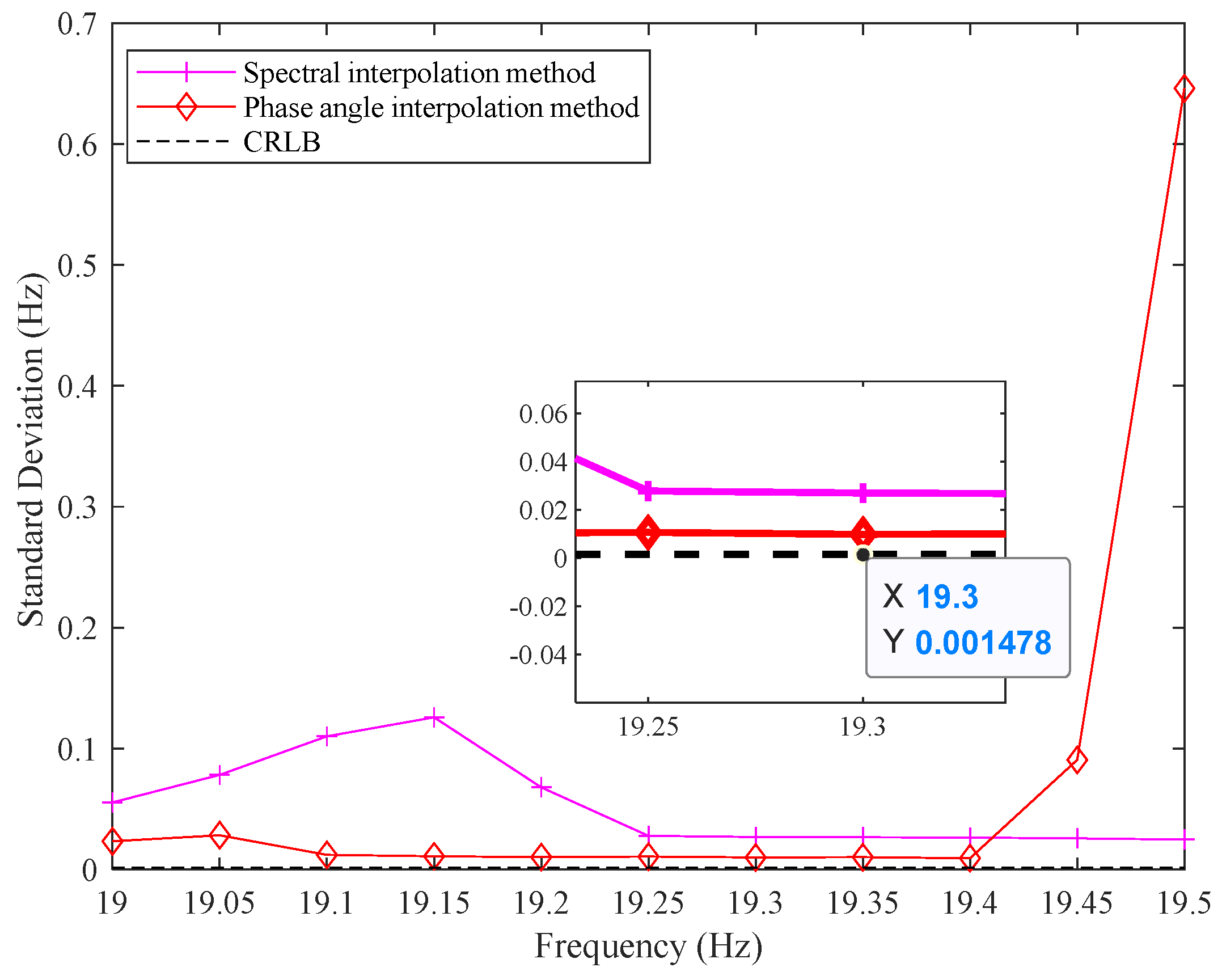
In order to analyze the correction ability of the phase angle interpolation method proposed in this paper to the frequency estimation value, we calculated the corrected frequency using the formula (10). Then, the estimated standard deviation of the phase angle interpolation method is compared with the spectral interpolation method of the Rife algorithm

$${\widehat{f}}_0=\frac{\left(k_1+r_1{\delta }_1\right)f_s}{N},$$

(10)

where, $f_s$ is the sampling frequency.

The comparison results of two different interpolation methods are shown in Figure 1. Compared with the spectral interpolation method, the phase angle interpolation has better anti-interference performance, which reduces the estimation error of the Rife algorithm when the estimated frequency point is close to the quantized frequency. However, since the phase angles at $k_1\pm 1$ are approximately equal, when the estimated frequency point is located in the center area of the two quantized frequency points, the correction direction in this area is easily misjudged, and the frequency estimation error is increased. We analyzed that there is an optimal correction interval for the frequency deviation factor in the phase angle interpolation mode, which is expressed as $0.1\le {\delta }_1\le 0.4$. When $0\le {\delta }_1<0.1$, due to the influence of noise, the optimal estimation performance is not achieved. When $0.4<{\delta }_1\le 0.5$, the correction direction is prone to misjudgment, the error is increased.

We also introduced CRLB (Cramer–Rao lower bound) in the comparison process. It defined the lower bound on the standard deviation of the frequency estimate for the optimal method:

$$St{d}_{CRLB}=\frac{1}{2\pi }\sqrt{\frac{12f_s^2{S}_s}{S_{n}N\left(N^2-1\right)}},$$

(11)

where, $S_s$ is the signal power, $S_n$ is the noise power.

Based on the above analysis, further optimization directions are proposed in this paper, which will be described in detail in the following subsection.

3.3. Shifted the Frequency

We have obtained the optimal correction interval under the phase angle interpolation method. Therefore, the frequency estimation method will be optimized using the frequency shift technique.

Foremost, the estimation threshold of the frequency deviation factor is set, i.e., the upper threshold $V_{down}=0.4$, and the lower threshold $V_{up}=0.1$. Then, the threshold judgment is performed on the frequency deviation factor obtained by formula (8). If the frequency deviation factor is within the decision threshold, the signal frequency can be estimated directly using Formula (10). Otherwise, the signal needs to be shifted to the left or right by ${\delta }_k$ quantized frequency units according to the correction direction $r_1$, and the signal is moved to the optimal estimation interval.

The frequency shift factor is expressed as

$${\delta }_k=0.3-{\delta }_1.$$

(12)

After the frequency shift of the signal, DFT is performed again to calculate the spectrum:

$$F^{\prime }\left(k\right)={\left(-1\right)}^M{\left(M!\right)}^2\frac{AN}{2}\frac{\sin \left[2\pi \left(k-k_0+r_1{\delta }_k\right)\right]}{\pi {\displaystyle \prod _{n=-M}^M\left(k-k_0+n+r_1{\delta }_k\right)}}.$$

(13)

Secondly, the phase angles of the $F^{\prime }\left(k_1\right)$ and $F^{\prime }\left(k_1\pm 1\right)$ are calculated using the phase angle function $angle(·)$, and the phase angles of $F^{\prime }\left(k_1+1\right)$ and $F^{\prime }\left(k_1-1\right)$ are compared again to determine the correction direction $r_2$ after the frequency shift. Eventually, the Formula (8) is used to determine the frequency deviation factor ${\delta }_2$ after the frequency shift. The calculation method of the signal frequency is expressed as

$${\widehat{f}}_0=\frac{\left(k_0+r_2{\delta }_2-r_1{\delta }_k\right)f_s}{N}.$$

(14)

3.4. PAI–Rife Algorithm

Based on the contents of three subsections, A, B, and C, an improved algorithm is sorted out, namely the PAI–Rife algorithm. The proposed algorithm is divided into signal windowing, phase angle interpolation, and frequency shift optimization. The spectrum leakage, judgment of correction direction, and interpolation method are optimized, respectively. The calculation process of the PAI–Rife algorithm is given in Algorithm 1.

The operation process of the PAI–Rife algorithm is briefly described as follows:

• The Rife–Vincent (I) window is added to the signal, and an N-point DFT calculation is performed to obtain the signal spectrum.
• Using the phase angle function to calculate the phase angle $P_1$ corresponding to the maximum spectrum and the phase angles $P_2$ and $P_3$ corresponding to the adjacent two spectrums.
• By comparing the sizes of $P_2$ and $P_3$, the correction direction $r_1$ and the frequency deviation factor ${\delta }_1$ are preliminarily determined. Assuming $P_2=angle\left[F^{\prime }\left(k_1-1\right)\right]$, if $P_2>P_3$, interpolation will be performed on the left of the maximum spectrum, at this time $r_1=-1$. If $P_2<P_3$, then the actual frequency point is considered to be on the right of the maximum spectrum, at this time $r_1=1$.
• A threshold decision is made on the frequency deviation factor ${\delta }_1$. If $0.15\le {\delta }_1\le 0.35$, the formula (10) is used to calculate the frequency. Otherwise, go to step 5.
• The signal frequency is shifted by ${\delta }_k$ quantized frequency units, and steps 2 and 3 are repeated to determine the correction direction $r_2$ and the frequency deviation factor ${\delta }_2$. The final frequency is calculated using Formula (14).

Algorithm 1: The proposed PAI–Rife Algorithm
Input: Output: Initialize:	A sinusoidal signal $s\left(n\right)$ Frequency estimation ${\widehat{f}}_0$ Windowing $\hspace{1em}\hspace{1em}\hspace{1em}\hspace{1em}\hspace{1em}\hspace{1em}\hspace{1em}x\left(n\right)=s\left(n\right)h\left(n\right)$
Step 1:	Get the position of the maximum spectral $\hspace{1em}\hspace{1em}\hspace{1em}\hspace{1em}\hspace{1em}\hspace{1em}{k}_1=\max \left(\left|FFT\left\{x\left(n\right)\right\}\right|\right)$
Step 2:	Calculate $FFT\left\{x\left(k_1\right)\right\}$ and $FFT\left\{x\left(k_1\pm 1\right)\right\}$
Step 3:	Calculate the phase angles $P_1$, $P_2$ and $P_3$ at $k_1$, $k_1+1$ and $k_1-1$ with phase angle function $angle(·)$
Step 4:	Calculate correction direction and frequency deviation If $P_2>P_3$ $r_1=1$ ${\delta }_1=\frac{P_1}{P_1+P_2}$ Else $r_1=1$ ${\delta }_1=\frac{P_1}{P_1+P_3}$ End of if
Step 5:	Frequency shift If $0.1\le {\delta }_1\le 0.4$ ${\widehat{f}}_0=\frac{\left(k_1+r_1{\delta }_1\right)f_s}{N}$ Else $x^{\prime }\left(n\right)=x\left(n\right)e^{\frac{j2\pi r_1\left(0.3-{\delta }_1\right)n}{N}}$    Go to Step 1 $\hspace{1em}\hspace{1em}{\widehat{f}}_0=\frac{\left(k_1+r_2{\delta }_2-r_1\left(0.3-{\delta }_1\right)\right)f_s}{N}$ End of if Return ${\widehat{f}}_0$

4. Simulation Analysis

4.1. Experimental Methods

The MATLAB simulation platform is used to simulate and analyze the PAI–Rife algorithm. Computational complexity, mean, standard deviation, and misjudgment rate of correction direction are used as evaluation indicators to compare with Rife [15], CQRE [25], ASIQ–Rife [26], An–Rife [27] algorithms. Meanwhile, the mean and standard deviation of PAI–Rife are compared with other frequency domain estimation algorithms, such as HAQSE [21] and T-PP [22]. In the simulation process, additive white Gaussian noise with a mean of zero is added to the signal, and the CRLB is introduced as an index for estimation accuracy. The specific simulation parameters are shown in

Table 1. Simulation parameters.

Parameters	Value
Monte Carlo times	10,000
Sampling points ($N$)	1024
Quantization frequency ($f_0$)	19 Hz
Sampling frequency ($f_s$)	1024 Hz
Frequency resolution ($△f$)	1 Hz
SNR	−10 dB:2 dB:10 dB

.

4.2. Computation Complexity

It is known that the number of complex multiplications required by the Rife algorithm to perform an N-point FFT operation is

$$C_M=\frac{N}{2}\log \left(N\right),$$

(15)

and the number of complex additions is

$$C_A=N\log \left(N\right),$$

(16)

where, $\log (·)$ is the base 2 logarithmic operation.

During the simulation, $2N$ complex multiplications and $2\left(N-1\right)$ complex additions are required to compute the maximal and submaximal spectra. The signal frequency shift also required $N$ complex multiplications. In the PAI–Rife algorithm, the probability that the signal is frequency shifted is 40%. Therefore, the algorithm increased the computational quantity compared to the Rife algorithm by $0.4\left(N+2N\right)=1.2N$ complex multiplications and $0.4\left(2\left(N-1\right)\right)=0.8\left(N-1\right)$ complex additions. The computation complexity of different Rife algorithms is shown in

Table 2. Complexity of different Rife algorithms ($N=1024$ ).

Algorithm	Complex Multiplications	Complex Additions	Computation Points	Increased Complexity
Rife	$C_M$	$C_A$	15,360.0	0%
ASIQ–Rife	$C_M+8N$	$C_A+5.3(N-1)$	28,973.9	88.6%
An–Rife	$C_M+5N$	$C_A+3.3(N-1)$	24,265.1	55.3%
CQRE	$C_M+2N$	$C_A+2(N-1)$	19,454.0	26.7%
PAI–Rife	$C_M+1.2N$	$C_A+0.8(N-1)$	17,407.2	13.3%

.

The computational complexity of several Rife algorithms is listed in Table 2. Although the ASIQ–Rife algorithm does not need its frequency shifted, the Rife and Quinn algorithms are used many times during its computation, resulting in a significantly increased computational complexity. The An–Rife algorithm required two frequency shifts, and the probability of being frequency shifted for the second time is 66%, resulting in a 55.3% increased amount of computation. The CQRE algorithm only needs to perform a spectral peak search again, so the increased amount of calculation is slight. In the estimation process of the PAI–Rife algorithm, the spectrum is recalculated only after the frequency shift, and the probability of the frequency shift is only 40%, so the calculation amount is much smaller than the other three improved algorithms. Compared with the CQRE algorithm, the calculation amount is reduced by 13.4% while improving the performance.

In addition, we counted the single simulation time of the PAI–Rife algorithm. From the time the signal is received to the end of the estimated frequency, the total is 0.574 ms. It is enough to show that the PAI–Rife algorithm can estimate the signal frequency in real-time and meet the needs of the IoT for real-time monitoring of structural status, positioning, and tracking.

4.3. Estimated Performance at Different Frequencies

In this subsection, the estimation performance of the PAI–Rife algorithm at different frequencies is tested. The quantization frequency $f_0=19 \mathrm{Hz}$ is set, $0.05\Delta f$ is the quantization interval, and 11 quantization frequency points $f_i$ are taken between $\left(f_0\sim f_0+\Delta f/2\right)$. The SNR is −6 dB.

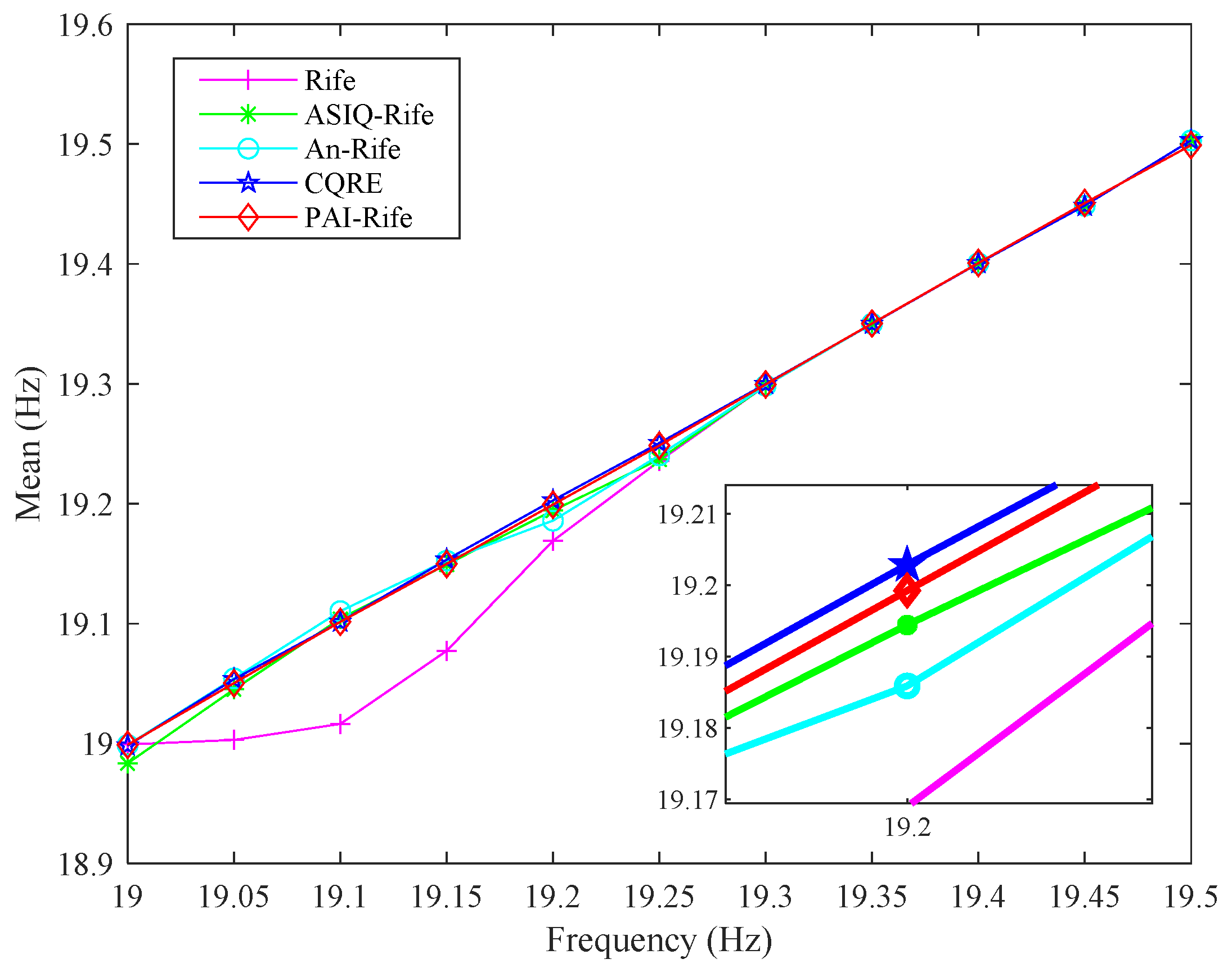
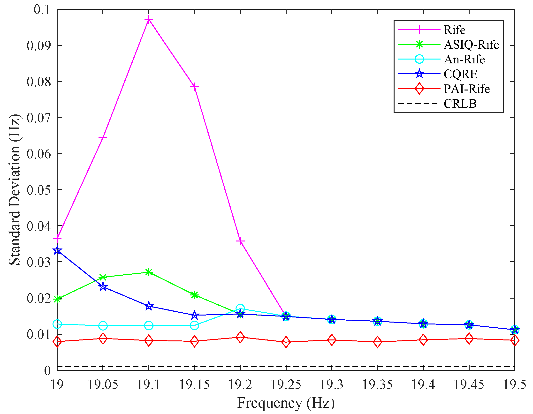
The comparison results of PAI–Rife and several other Rife algorithms are shown in Figure 2 and Figure 3. The estimation error of the Rife algorithm is substantial near the quantization frequency. The ASIQ–Rife, An–Rife, and CQRE algorithms have been improved to reduce the estimation error near to the quantization frequency. However, they have not changed the spectral interpolation method of the Rife algorithm. Therefore, the estimation accuracy in the optimal interval is the same. The PAI–Rife algorithm proposed in this paper changed the interpolation method and designed the judgment basis for the correction direction, making the estimation of the frequency deviation factor more accurate. At the same time, a more reasonable and accurate decision threshold is set, and the signal frequency is shifted to the optimal estimation interval, which makes the performance of frequency estimation more stable.

According to the statistics of standard deviation results, the mean value of the standard deviation of the Rife algorithm on 11 frequency points is about 0.029. The mean value of the standard deviation of the better-performing An–Rife algorithm among the three existing improved algorithms is about 0.013. The mean value of the standard deviation of the proposed PAI–Rife algorithm is about 0.008. Therefore, the frequency estimation accuracy of the PAI–Rife algorithm has been dramatically improved, which is 38.5% higher than that of the An–Rife algorithm. The signal frequency can be calculated with better estimation accuracy than the other four algorithms at different frequency points.

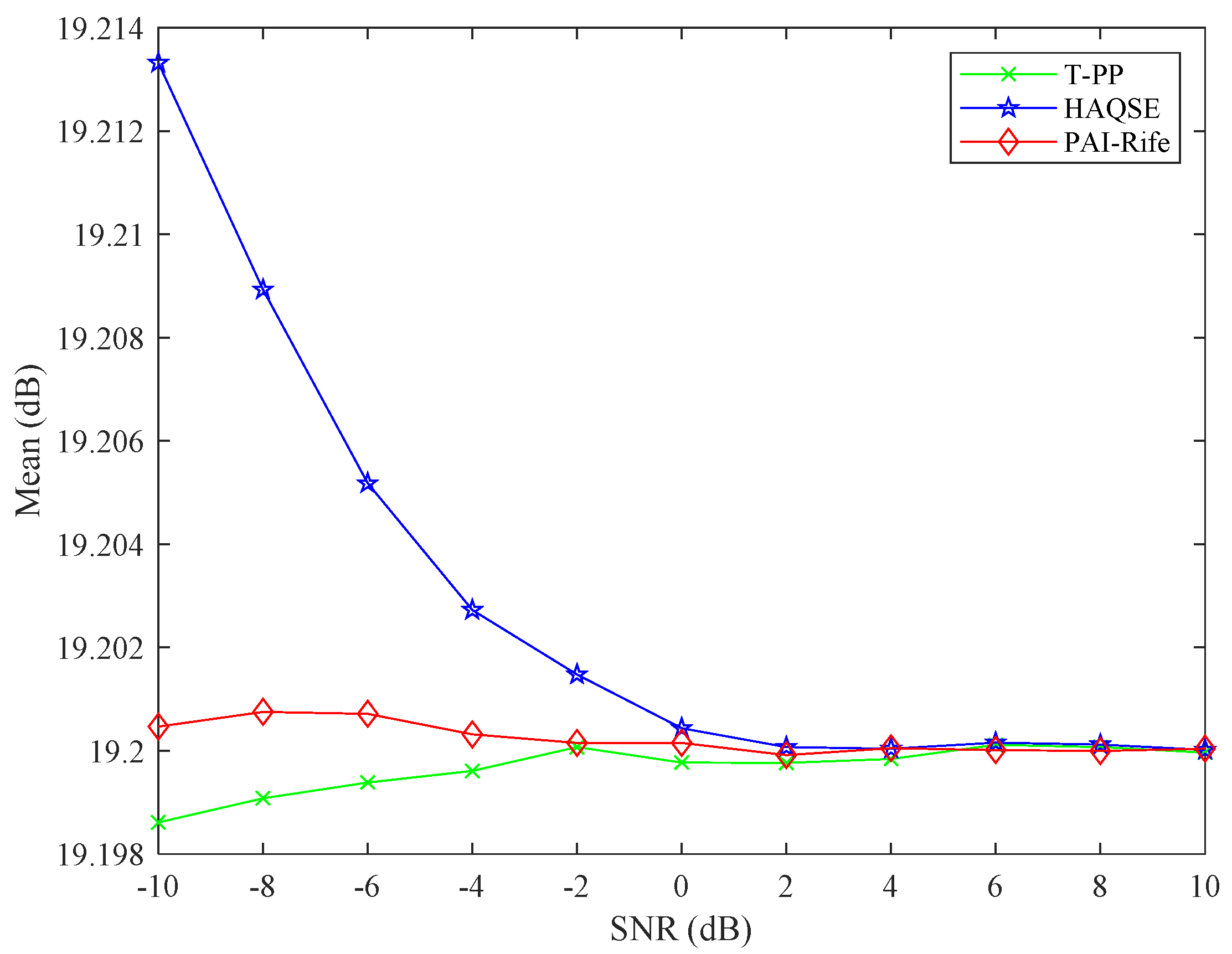
After comparing several Rife algorithms, we also conducted a comparative analysis under the same conditions with other frequency domain estimation algorithms, such as T-PP and HAQSE. The comparison results are shown in Figure 4 and Figure 5. Since the estimation error of the PAI–Rife algorithm and these two algorithms at different frequencies is small, the mean is relatively close. We conclude from the partially enlarged image of Figure 4 that the mean value calculated by PAI–Rife is closer to the actual frequency. With the change of the quantization frequency points, the standard deviation of the PAI–Rife algorithm is the smallest, and the estimation performance is the most stable. At the same time, since the phase angle interpolation is used, its frequency deviation correction ability is improved, and the estimation accuracy of different frequencies is better than the other two algorithms.

4.4. Estimated Performance at Different SNRs

The previous subsection analyzed the estimation performance of several algorithms for different frequencies. This subsection will investigate the interference of noise on frequency estimation. The quantization frequency point $f_i=19.2 \mathrm{Hz}$ is set. The comparison results with other Rife algorithms are shown in Figure 6 and Figure 7.

We can conclude that since the ASIQ–Rife, An–Rife, and CQRE algorithms are improved in different ways, the estimation accuracy at low SNR is improved. Our proposed PAI–Rife algorithm changes the traditional spectral interpolation method to the phase angle interpolation method. It used the stability of the phase angle to reduce the influence of noise on the signal. Therefore, the PAI–Rife algorithm’s mean of frequency estimation is the most stable in the environment with different SNRs.

It is calculated that the mean value of the standard deviation of the Rife algorithm is about 0.063. The CQRE algorithm performed the best among the three modified Rife algorithms, with a mean value of the standard deviation of about 0.02. The mean value of the standard deviation of the PAI–Rife algorithm is about 0.012. Compared with the CQRE algorithm, the anti-noise performance of the PAI–Rife algorithm is improved by 40%. The anti-noise performance is better than Rife, ASIQ–Rife, An–Rife, and CQRE algorithms. Especially in a low SNR environment, the improvement is more significant. The standard deviation is relatively closer to the CRLB.

The comparison results between the PAI–Rife and other frequency-domain estimation algorithms under different SNRs are obtained from Figure 8 and Figure 9. Due to the increased number of iterative computations, the length of the signal estimated by the HAQSE algorithm is limited. As the signal length increased, the estimation accuracy of the HAQSE algorithm gradually decreased. Therefore, in the low SNR environment, the estimation performance of the HAQSE algorithm is the worst. The PAI–Rife algorithm estimated a more precise frequency deviation factor through the proportional relationship between the phase angles. The estimated frequency value is closer to the actual frequency, which is not affected by the length of the signal.

4.5. Correction Direction Misjudgment Rate

There are two reasons for the error in frequency estimation: one is that the estimate of the frequency deviation factor is not accurate enough, and the other is that the correction direction is misjudged. In this subsection, the influence of the frequency deviation factor on the frequency estimation is analyzed, and the judgment results of the correction direction will be compared. Because the two frequency domain estimation algorithms of HAQSE and T-PP do not judge the correction direction, we only compared the misjudgment situation of PAI–Rife with Rife, ASIQ–Rife, An–Rife, and CQRE algorithms under different SNRs.

From the previous analysis of the frequency estimation algorithm, it can be seen that when the frequency point is close to the quantized frequency, the correction direction misjudgment rate of the Rife algorithm is relatively large, increasing the frequency error after frequency deviation correction. For the ASIQ–Rife algorithm, it judged the correction direction again after the signal frequency shift and reduced the misjudgment rate. Due to the improvement of the correction direction judgment method of the Quinn algorithm, the correction ability of the An–Rife algorithm has been optimized. The misjudgment rate of the CQRE and PAI–Rife algorithms are almost the same, and both have been significantly reduced. The reason is that the two methods of judging and correcting the direction are combined, which makes up for the shortcomings of the CQRE algorithm. For the PAI–Rife algorithm, we shifted the signal frequency to the best estimate range and used a phase angle less susceptible to noise to determine the direction of correction. Therefore, in the low signal-to-noise ratio environment, the accuracy of the correction direction judgment of the CQRE and PAI–Rife algorithms has been improved. After the analysis, it is concluded that under the condition of strong noise, the misjudgment rate of the correction direction of the PAI–Rife algorithm is very close to zero, which is much lower than that of the Rife, ASIQ–Rife, and An–Rife algorithms (Figure 10).

4.6. Analysis of Actual Measurement Data

We used an FMCW (Frequency Modulation Continuous Wave) radar sensor to obtain actual data of five different distances and further verified the estimation accuracy of the PAI–Rife algorithm. In addition, we estimated the frequency of the echo signal using the PAI–Rife algorithm. The estimated value of the distance is obtained by

$$R=\frac{cT{f}_e}{2B},$$

(17)

where, $T=N/f_s$ is the sampling period, $c=299,792,458 \mathrm{m}/\mathrm{s}$ is the speed of electromagnetic waves, $B$ is the signal bandwidth.

The measurement environment is a closed room. The radar is placed horizontally with the launch panel facing the roof. The distance data between the radar and the roof is obtained, and the data are sent to the terminal through serial communication. Before the measurement, the sampling frequency of the FMCW radar is set to $f_s=92.7835 \mathrm{KHz}$, the signal bandwidth $B=999.47 \mathrm{MHz}$, and the sampling number $N=1024$. The actual distances measured by the radar are 2097 mm, 2378 mm, 2420 mm, 2561 mm, and 2653 mm. Above all, the frequency estimation algorithm is used to estimate the beat frequency of the radar, and then the distance value is calculated. The results obtained by different Rife algorithms are shown in

Table 3. Comparison of distance values obtained by different algorithms.

Algorithm	2097 mm		2378 mm		2420 mm		2561 mm		2653 mm
	Results	Bias	Results	Bias	Results	Bias	Results	Bias	Results	Bias
Rife	2095.8	1.2	2320.3	57.7	2476.1	56.1	2587.5	38.9	2610.3	42.7
ASIQ–Rife	2095.8	1.2	2321.0	57.0	2475.8	55.8	2587.5	26.5	2614.4	38.6
An–Rife	2095.6	1.4	2321.0	57.0	2472.9	52.9	2591.8	30.8	2614.1	38.9
CQRE	2095.6	1.4	2323.4	54.6	2453.8	33.8	2581.6	20.6	2630.7	22.3
PAI–Rife	2097.1	0.1	2364.1	13.9	2413.8	6.2	2565.9	4.9	2652.5	0.5

. From the bias in the table, it can be concluded that for these five different distance data, the Rife algorithm has the worst estimation ability. Compared with the other four algorithms, the results obtained using the PAI–Rife algorithm are closer to the actual distance. In terms of distance estimation accuracy, the error rate of PAI–Rife is only 0.2%.

5. Conclusions

The signal input of IoT wireless sensors is often affected by noise, resulting in data loss from the original signal and the inability to access and correctly estimate the signal frequency. Spectral leakage and fence effects are issues that must be addressed when estimating frequency using a single-sensor approach based on signal processing. Among such algorithms, the Rife algorithm is widely used in microcontrollers of wireless sensors because of its simplicity and ease of implementation. Nevertheless, it is susceptible to noise and has limitations on the frequency range. To address this problem, we proposed the PAI–Rife algorithm. The main innovation of this algorithm is that it overturned the original frequency deviation factor and redefined it. Then, the traditional spectral interpolation method of the frequency estimation algorithm is improved with the help of the stable characteristic of the phase angle, the anti-noise performance of the algorithm is enhanced, and the frequency estimation accuracy is improved. The PAI–Rife algorithm met the needs of real-time monitoring of the IoT with low complexity and ensured the validity of the frequency information of wireless sensors.

Based on the Rife algorithm, the computational complexity of the PAI–Rife algorithm is only increased by 13.3%, which is much lower than the other three improved Rife algorithms. Moreover, while maintaining low computational complexity, the anti-noise performance is enhanced by 80.3%, and the frequency estimation accuracy is improved by 72.4%. The PAI–Rife algorithm proposed in this paper balanced the computational complexity and estimation accuracy. Its estimation performance is better than Rife, ASIQ–Rife, An–Rife, CQRE, HAQSE, and T-PP algorithms. Unfortunately, we did not test the proposed algorithm in the sensor communication link due to time constraints. In further work, we will realize the application in the communication link and complete the technical advancement from acquisition to transmission. At the same time, continuing to optimize the frequency estimation performance of the algorithm in a lower SNR environment to meet the practical application of the IoT in a more severe environment.