Automatic Failure Modes and Effects Analysis of an Electronic Fuel Injection Model

Abstract

In the development of safety-critical systems, it is important to perform failure modes and effects analysis (FMEA) to identify potential failures. However, traditional FMEA activities tend to be considered difficult and time-consuming tasks. To compensate for the difficulty of the FMEA task, various types of tools are used to increase the quality and the effectiveness of the FMEA reports. This paper explains an automatic FMEA tool that integrates the model-based design (MBD), FMEA, and simulated fault injection techniques in a single environment. The automatic FMEA tool has the following advantages compared to the existing FMEA analysis tool: First, the automatic FMEA tool automatically generates FMEA reports, unlike the traditional spreadsheet-based FMEA tools. Second, the automatic FMEA tool analyzes the causality between the failure modes and the failure effects by performing model-based fault injection simulation. In order to demonstrate the applicability of the automatic FMEA, we used the electronic fuel injection system (EFI) Simulink model. The results of the automatic FMEA were compared to those of the legacy FMEA.

1. Introduction

In safety-critical fields such as automobiles, aerospace, and railways, it is important to comply with the international standards or guidelines for functional safety to prevent harm caused by potential system failures. Industries employ their own standards, such as SAE ARP 4754A/4761A and RTCA DO-178C/DO-254 for aerospace, or ISO26262 for the automotive industry [1,2,3,4,5,6]. The purpose of these guidelines is to identify hazards and decrease the occurrence of accidents to socially acceptable levels. HAZOP (hazard and operability analysis), FMEA (failure modes and effects analysis), and FTA (fault tree analysis) activities are key to achieving these goals [7,8,9,10]. Among them, FMEA investigates the causality of faults and failures to improve the safety and reduce the likelihood of recall. However, traditional FMEA activities tend to be considered difficult and time-consuming tasks, so the effectiveness of the results falls short of expectations [11,12].

To facilitate FMEA tasks, various types of tools are used to increase the quality and the effectiveness of the FMEA reports. Traditional FMEA analysis tools use spreadsheet-based FMEA templates [13,14,15,16]. The spreadsheet-based FMEA tool provides users with the FMEA templates according to the regulations or specifications agreed upon by the stakeholders in their field. Then, the users identify each potential failure mode and assess their local and global failure impacts on safety, including the severity of the occurrence. Meanwhile, the complexity of software in electric equipment has increased rapidly, making it very difficult to analyze system fault–failure causalities and their impacts [17]. To address these challenges, leading organizations are pursuing model-based SW development, including UML, SysML, and Simulink [18,19,20,21,22,23,24].

Model-based FMEA techniques use design models to support a visible and automated analysis environment. In model-based design (MBD), the design model describes the function of the system and its behavior by utilizing graphical objects of various types [25,26,27,28,29,30,31,32,33]. The MBD and FMEA processes can be integrated to simulate the failure effects at the various levels, from the local level up to the vehicle or system level [21]. This approach can evaluate the fault–failure causality for a limited number of cases [34,35]. In addition, FMEA users expect support for the risk priority number (RPN) to respond to unacceptable failure effects.

This paper explains an automatic FMEA tool that integrates the MBD, FMEA, and simulated fault injection techniques in a single environment. The automatic FMEA investigates the fault–failure causality of the system using simulated fault injection to find the potential failure modes and their effects at various levels, from local to global. In addition, it incorporates an AI-based failure effect classification module to identify the severity and occurrence rate so that the risk priority matrix can be automatically presented. In addition, the automatic FMEA is based on MATLAB/Simulink to support large numbers of users in safety-critical fields around the world.

The automatic FMEA tool has the following advantages compared to the legacy FMEA tools as well as the model-based FMEA tools: In the legacy FMEA, the users are responsible for the creation of the FMEA report, but in the automatic FMEA, the tool produces it and the user only needs to review the contents of the FMEA results [13,14,15,16]. The legacy FMEA tools provide the FMEA templates, and users enter the entries of the FMEA table using design documents and safety guidelines. The automatic FMEA tool generates FMEA results by analyzing the failure effects due to failure mode, using the integrated FMEA environment with model simulation and simulated fault injection.

Compared to other model-based FMEA tools, the automatic FMEA tool analyzes the failure effects systematically by using the integrated FMEA environment, where the injection mechanism utilizes the saboteur fault injection module. While the existing model-based FMEA tools can analyze the failure effects using the model simulation process, they can only perform for a limited number of cases. The automatic FMEA tool performs fault injection simulation using the saboteur fault injection block, which supports the HAZOP-guidewords-based fault modeling. This feature enables it to create a large number of test cases and identify their fault–failure causalities as well as the associated RPN figures using the fault injection campaign plan.

In order to demonstrate the effectiveness of the automatic FMEA, we developed a prototype using the C# programming language, and performed a case study using the electronic fuel injection Simulink model [36]. We explained the results of the automatic FMEA and compared them to those of the legacy FMEA tool.

The rest of this paper is organized as follows: Section 2 explains the trends of FMEA analysis support tools and model-based FMEA analysis technology. Section 3 describes the automatic FMEA environment, support technologies, and analysis procedures. Section 4 presents an MILS test model and an FMEA report developed to check the performance of the automatic FMEA. Finally, Section 5 presents the significance of automatic FMEA research and future research plans.

2. Failure Mode–Failure Effects Trends

Safety certification guidelines (ARP4761, ISO26262, etc.) require safety analysis documents and data of FMEA and FTA that can be reviewed by the certification authorities or their representatives. The safety analysis process is a time- and resource-consuming task that requires safety engineering technology as well as domain knowledge. FMEA is a process of reviewing thousands of pages of development documents and identifying the potential failure sources and their effects in a detailed manner. In addition, the developer must iterate this safety analysis process when there is a modification due to a requirement change or design error.

The legacy FMEA analysis tools generally use the templates required by the corresponding safety specifications [13,15,16,37,38]. These tools record the failure modes and their effects manually as well as calculating the criticality, which is the product of the occurrence probability and the severity. Unfortunately, as the size of modern cyber-physical systems or embedded targets is growing rapidly, it is becoming more difficult to create the FMEA reports. The representative template-based FMEA analysis tools include IQ-FMEA, ENCO, and Relex [7].

As model-based development technology has become popular in the SW development process, research on model-based FMEA has increasingly taken place [39]. Using the design model developed in the MBD process, the model-based FMEA applies the failure mode to the design model and performs the model simulation to produce the possible failure. Like the traditional FMEA, the model simulation can generate the failure effects at three levels: the local effect, the next effect, and the end effect.

The advantages of model-based FMEA (MB FMEA) are as follows: (1) It is relatively easier to perform risk analysis tasks than existing spreadsheet/Excel-based FMEA tools, thanks to simulation. The role of the members of the FMEA committee changes from producing FMEA reports to reviewing reports. (2) The MB FMEA method has the advantage that developers can minimize cost and time, and maximize efficiency. In one study, the use of automated development tools was reported to increase ROI by 2500% [40]. In the legacy FMEA method, the absence of an FMEA staff member means suspension of work. However, in the model-based FMEA method, risk analysis can be performed using simulation in advance, and the staff member can proceed with the task by checking the results later. (3) Using the MB FMEA method, it is possible to consistently and objectively evaluate various types of failure modes using simulations. In the legacy FMEA method, there is the problem that the FMEA staff may make a subjective evaluation.

Many studies are being conducted on MB FMEA using SysML, Modelica, Simulink, and fuzzy inference engines [21,25,26,27,28,29,30,31,32,33,34]. Among them, we explain the HiP-HOPS FMEA tool and the MADe FMEA tool. The HiP-HOPS FMEA tool automatically analyzes the Simulink model, identifies FTA synthesis and fault modes, and creates FMEA tables [21]. In the process of creating an FTA, the analysis model is optimized with a minimal cut set. However, each failure dataset (fault rate, failure effects, etc.) must be directly entered, and there are limitations in analyzing severity, incidence, and detection, which are essential for FMEA analysis. MADe FMEA is a commercial FMEA analysis tool that performs model-based failure mode derivation and failure impact analysis by defect injection simulation [34]. In addition, it is possible to establish an integrated safety/reliability analysis environment using the MADe tool. However, it uses its own modeling language, so the general users must undergo a significant learning period.

Automatic FMEA is a systematic failure analysis environment using statistical fault injection simulation and rule-based failure classification. The automatic FMEA is built on top of the statistical fault injection environment. Once it sets the statistical confidence level, it automatically calculates the number of faults to be injected, and builds the fault list using the HAZOP guidewords. After the injection campaign, all failure information is stored and processed to assess the severity of each injection event using rule-based inference.

Table 1. Comparison of various types of FMEA tools.

Features	Automatic FMEA	HiP-HOPS	MADe	Relex
Environment	Simulink	Simulink	MADe FMEA	Spreadsheet SW
Failure Assessment	Automatic	Semi-automatic	Automatic	Manual
Failure Effects Analysis	Fault injection simulation	Manual simulation	Fault injection simulation	Manual
Severity	Rule-based system	FTA	User manual
Occurrence		FTA	MADe-FTA
Detection		N/A	N/A
Fault Injection Mechanism	Saboteur	N/A	Mutation	N/A

shows the comparison of the features of the automatic FMEA tool to those of the model-based FMEA tools as well as the legacy FMEA tool.

The advantages of our tool compared to other model-based FMEA tools are as follows: First, Automatic FMEA uses saboteur modules to express a fault model, so it performs a fault injection simulation more efficiently than other tools. For example, a mutation-based fault injection method requires input/output each time a large number of mutants are built, managed, and simulated, so the simulation overhead is relatively larger than the load required for saboteur-based simulation [41]. Second, the saboteur module of automatic FMEA expresses the failure model using HAZOP guidewords. Accordingly, various failure modes of FMEA may be conveniently and without omission. This can be found in Section 3.2. Third, we can derive objective results because we use rule-based systems to determine the effects of failures. We developed a GUI for entering the condition part and the action part of the rule for domain experts. The knowledge of domain experts can be used as a criterion for determining failure effects. This can be found in Section 3.2.3.

3. Automatic FMEA System

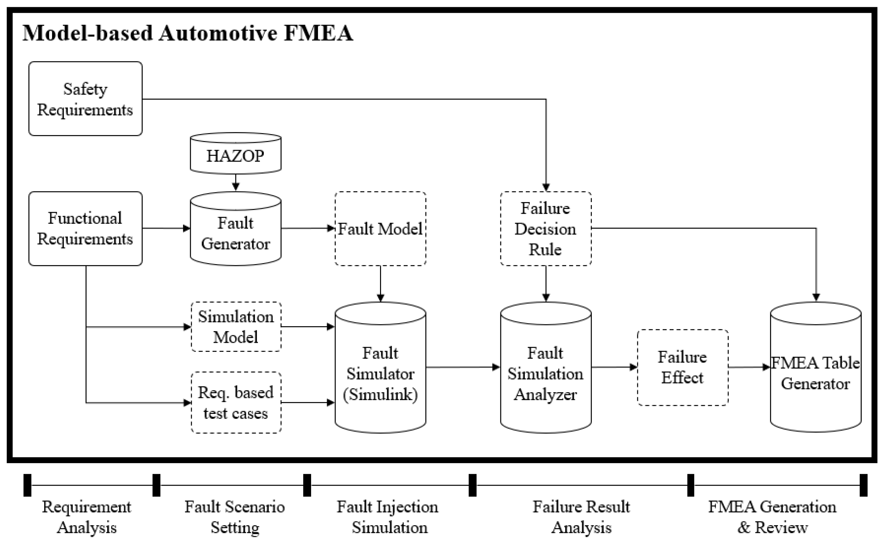
3.1. Automatic FMEA

Automatic FMEA is a safety analysis tool that performs fault simulation in a Simulink environment to evaluate the failure effects of the design target system. Automatic FMEA restructures the Simulink model to perform fault simulation. The Simulink model consists of hierarchically connected functional blocks. In Simulink, one can express the algorithm using the block, which is an MDL file in the Simulink internal system. Automatic FMEA parses the Simulink MDL file to restructure into a suitable model for the fault injection process. In the restructured model, we insert a saboteur block between the original system blocks so that it can perform the fault injection simulation. We explain the internal process of the automatic FMEA shown in Figure 1. First, we use the safety requirements and design documents of the target system to identify the range of tolerance of the design parameters of the system [2,4]. Using the results, we can identify the severity of the failure effects for the given failure modes, which is accomplished by injecting the corresponding faults into the target system.

Second, we create a fault model corresponding to the failure modes using the design parameters of the target models, and perform fault simulation to evaluate the failure effects. In the model-based design process using Simulink, the target model has to be verified using the Simulink Design Verifier. After this process, the fault models are built using the selected HAZOP guidewords corresponding to the design parameters of the target model. During fault injection simulation, we inject these fault models representing a specific failure mode, and record the results of the fault simulation, which are used to identify the failure effects.

Third, using the results of the fault simulation, we build the failure information that can be used for the FMEA report. Using the results of the fault simulation, it is possible to identify the local effect, the next effect, and the end effect of the given failure modes. Moreover, using the failure decision rules, we can identify the failure effects, which are the severity and occurrence rate of the failure modes. Using these as the information, we may build the preliminary FMEA report that can not only accelerate the FMEA process, but also be used to find the unidentified failure modes by the FMEA committee members, which may happen in the case of a new system’s development.

In order to develop automated FMEA analysis tools in the Simulink environment, it is necessary to establish solutions to three development problems: The first is “How to track the failure impact of FMEA’s failure mode?” One of the purposes of FMEA analysis is to track the potential impact of the system due to failure. In the traditional FMEA process, the knowledge and experience of the member of the FMEA committee are important for the identification of the failure. In model-based development, the model itself can be used as a tool to track the impact of failure. Automatic FMEA uses a Simulink model tree generation algorithm to trace the impact of failure in the model. This is described in detail in Section 3.2.1.

The second problem is “How to apply the failure mode to the simulation model?” Automatic FMEA uses the fault simulation corresponding to the failure mode to derive information necessary for the completion of the FMEA report. The fault simulation is implemented using the saboteur technique. This is explained in detail in Section 3.2.2. Finally, the third question is “How to set the severity, detection, and occurrence of failure effects?” Experts allocate the severity, detection, and incidence of FMEA to values between 0 and 10, based on experience. However, automatic FMEA can quantify and allocate the severity and detection of failures using the result values of failure simulation. To this end, automatic FMEA proposes a method of analyzing simulation result values and determining severity detection using rules and rule engines. The degree of occurrence can be considered to be derived as a statistical defect injection test. Rule-based failure analysis is described in detail in Section 3.2.3.

3.2. The Function of Automatic FMEA

3.2.1. Simulink MDL Parser

The Simulink MDL parser identifies each block and its input/output ports in the Simulink design model, and derives connectivity and hierarchy information from among them. The Simulink MDL file specifies the system structure as a pair of keys and values [42]. When the Simulink specifies a functional unit block of Simulink, the model is configured with a key representing the type, name, and location of the block. Simulink uses three keys: the system syntax, the block syntax, and the line syntax, which is used to specify the connectivity and hierarchy of the design model. The system syntax consists of one or more blocks or subsystems in the Simulink model so that we can infer the hierarchical relationship between blocks. The block syntax and line syntax can interpret the connection relationships between each block in the Simulink model. Therefore, parsing the MDL file, we can identify the hierarchy and connection information of the blocks in the Simulink design model. Using this information, we can find the variables and their values to describe the local effect, next higher effect, and the end effect in the FMEA table.

The Simulink MDL parser receives the model of the MDL format as input, interprets the syntax, and outputs a Simulink model tree that can derive FMEA failure traceability analysis. The MDL parser consists of three stages: the keys and values classification stage, context interpretation stage, and model reconfiguration stage, as shown in Figure 2. In the first stage, the keys and values classification process identifies a key in the MDL file, and stores a valid key and its value. In Simulink, the MDL model is described using keys such as “system”, “block”, and “line” and their values. The Simulink MDL parser selects and stores only the information necessary for generating the Simulink model tree from the input file.

In the second stage, the context interpreter checks the block configuration and connection of the model, as well as the parent–child relationship structure of the block. The Simulink model uses the “system” key to define a parent block, including the best block or one or more functional blocks. Alternatively, signal connection between blocks is established using the “line” key and each block port’s information. The context interpreter checks the previously processed key and value set information to create a linked block set for Simulink model tree configuration. In the third stage, the model reconfiguration process creates a Simulink model tree that can be used to trace the fault propagation path using the linked block sets connected according to the system structure. The Simulink model tree created with the Simulink MDL parser is plotted in Figure 2. As shown in the figure, we can confirm the hierarchy, configuration, and the input/output between blocks of the Simulink design model.

Using the Simulink model tree, we can describe the propagation of the failure effects of the given failure mode, i.e., the local effect, next higher effect, and the end effect in the FMEA table. Figure 3 describes a method of deriving a failure effect from a Simulink model tree. The left side of the figure explains the inter-block failure propagation within the subsystem block, and the right side shows an example of the intra-block failure propagation between the blocks up to the parent block. We can set the initial faulty block to local effect, and identify the next higher effect and the end effect blocks using the inter-block link information. If the model has the hierarchy, we can append the intra-block link information to the previous failure propagation list so that the expanded failure propagation list can be obtained.

3.2.2. Saboteur-Based Fault Simulation Model Creation

Automatic FMEA builds a simulation model for the fault injection campaign to analyze the failure effects for given failure modes by applying the saboteur module to the Simulink MDL file. In the saboteur technique, we may append a saboteur block between the design blocks so that it can insert faults into the design model. The saboteur block converts the value of a variable into a faulty value according to a fault model specified by the fault injection campaign. The saboteur technique has the advantage of being able to create a failure test model in a simple manner. However, the process of adding saboteur blocks may alter the original functionality of the design model. In order to maintain the consistency between the original model and the fault simulation model, we perform a verification simulation using Simulink Design Verifier and the benchmark experiments, which compares the results of the simulation with and without the saboteur block in the design model.

The saboteur block of automatic FMEA injects a fault model from the set of faults listed from the fault injection campaign. The fault model illustrates the failure modes using (1) a fault model, (2) a fault occurrence time, and (3) a fault duration time. The fault model is constructed by applying a HAZOP guideword to each and every variable available in the Simulink design model. In automatic FMEA, we multiply the value of the design parameter of the Simulink model by the proportional coefficient using the failure keyword as shown in

Table 2. HAZOP-based failure modes.

Failure Keyword		Meaning
Loss of function (LF)		Functions not activated
Incorrect	More than requested (MTR)	Functions activated in excess of requested quantity
	Less than requested (LTR)	Functions activated in less than requested quantity
	Wrong direction (WD)	Reverse functions activated
Unintended activation of function (UAF)		Functions activated at unintended time
Locked/stuck function (SF)		Function is not updated
Timing	Early	Function activated earlier
	Late	Functions activated later

. For example, suppose the parameter “A” replies with the “less than requested” failure keyword. Then, it builds the three-fault model using 90%, 80%, and 70% of the value of the parameter “A” after the consultation with the domain experts. In this way, various types of failure effects may be investigated in a quantitative manner using the derived fault models, so that the automatic FMEA may contribute to discovery of the unseen failure mode by the members of the FMEA committee.

Automatic FMEA integrates the saboteur blocks with the blocks in the simulation models to facilitate the simulated fault injection campaign. Let us assume that a block in Simulink is connected with a port key and a line key, where the port key is an input or output identifier of a block, and the line key is a link of two blocks. Automatic FMEA searches for the port key and line key of the block corresponding to the fault injection location to add the saboteur block and modify its value. The original design model and the model prepared for the fault injection experiments are compared in Figure 4. The required number of the fault simulation design model is created, and the injection process proceeds automatically so that we may accumulate a large amount of the failure mode–failure effects relationship information for the Simulink design model. In the figure, a saboteur block is added between each block to implant a defect. Automatic FMEA performs the Simulink fault injection simulation of the preparation, execution, and the collection of the simulation log for the fault models described in the fault injection campaign.

Automatic FMEA controls the saboteur block added to the Simulink model to perform a failure simulation, as shown in Figure 5. In a normal case, the output from the front logic block is transferred to the back-end logic block via the correct data (CD) block. In the case of the fault injection simulation, one of the outputs of the failure data (FD) block is transferred to the back-end logic block according to the fault injection scenario.

The automatic FMEA controls the saboteur block using the MATLAB command script [43]. The MATLAB command script may probe or update the status of the block in the Simulink model. In addition, the breakpoint function may be used to pause and resume the simulation at a predetermined time or event. According to the failure scenario, automatic FMEA simulates failure in the following steps: (1) pause the current simulation run when the simulation time reaches the fault time, (2) set the failure data (FD), (3) resume the simulation, (4) pause the simulation after the fault duration time, (5) restore the original value, and (6) resume the simulation run. Automatic FMEA sets or releases the fault values using the failure mode selector and failure data values of the saboteur block. The failure mode selector of the saboteur block selects one of the six HAZOP fault types, and the failure data set the value of the fault model. For example, if the failure mode is that the sensor degrades and its signal is reduced to 70% of the nominal value, the failure mode selector enables the “Less Than Requested” mode and sets the failure data to 70%.

3.2.3. Rule-Based Failure Determination Function

Automatic FMEA uses rule-based engines to analyze the result of the fault injection simulation and determine the severity of the failure effects for the given failure mode. Automatic FMEA determines the effect of a failure mode by comparing the results of a golden run simulation to that of the fault simulation. In addition, it also examines the value, state, and condition of the parameter of the fault simulation.

The rules in the automatic FMEA are designed to support the fault models and the fault injection block shown in Figure 5. Each rule evaluates the failure mode and the value of the parameter. First, the condition part of the rules is designed to identify the failure mode of the current simulation, including (a) the underestimation values check for system degradation, (b) the overestimation values check for system overload, (c) the error margin check for the stability of a performance parameter, or (d) the failure event check for the detection of the specific failure effect.

Next, the action part of the rules is used to determine the value of the entries of the severity, occurrence, and controllability in the FMEA table. For the given failure mode, the automatic FMEA performs a large number of fault injection simulations to find the behavior of the failure effect. Thus, we can compare the distribution of the parameters from the current simulation runs to that of the golden run simulation so that the action part of the rule can assign the resulting severity between 0 and 10. The occurrence and detection entries of the FMEA table are not yet implemented, so it is necessary to have a meeting with the domain experts and the designers of the model. This process of identification of the severity, occurrence, and detectability of the failure effects is summarized in Figure 6.

3.2.4. Implementation of Automatic FMEA

The operation of automatic FMEA has four steps, as follows: (1) Simulink model analysis, (2) failure mode setting, (3) failure decision rule setting, and (4) fault injection simulation. The Simulink model analysis step analyzes the input Simulink design model, prepares an initial FMEA template, and performs a golden run simulation. In the failure mode setting step, one failure mode from the failure mode list is selected and injected into the design system. The failure effect determination rule setting step analyzes the fault simulation result and defines a rule for determining the severity. Fourth, in the failure injection simulation step, the fault injection simulation is automatically performed according to the previously set failure (operation) mode, and the result is analyzed according to the failure impact analysis rule. The screenshot of the automatic FMEA user interface and the final results are shown in Figure 7.

4. Case study: Electronic Fuel Injection System

4.1. Electronic Fuel Injection System

4.1.1. Overview of the Electronic Fuel Injection System

The electronic fuel injection (EFI) system is a system that calculates the amount of fuel injected into the engine. The EFI system may be described using the sensor, engine control unit (ECU), and engine, as shown in Figure 8. The sensor sub-system measures the engine state and transmits the measurement result to the ECU subsystem. The ECU subsystem calculates the amount of air and fuel using the sensor information. The engine subsystem generates the power of a vehicle through four-stroke cycles using fuel and air.

The sensor subsystem consists of four sensors: (1) The throttle position sensor (TPS) measures a throttle valve angle. (2) The crankshaft position sensor (CPS) measures the rotational speed per second of the crankshaft of the engine unit. (3) The exhaust gas oxygen sensor (EGO) measures the oxygen concentration in the exhaust gas. (4) The manifold absolute pressure sensor (MAP) measures the internal pressure of the intake manifold. The measured sensor data are connected to the data bus and transmitted to the ECU subsystem.

The engine control unit (ECU) subsystem calculates the amount of fuel by performing three processes from the input sensor subsystem data: First, the sensor data filter process checks whether there is any abnormality in the data received from the data bus. Second, the control logic process sets the air ratio using the verified sensor data and current vehicle state information. Third, the fuel rate calculator process calculates the amount of air intake using vehicle condition information and throttle position data, and calculates the amount of fuel based on the set air ratio.

The engine subsystem consists of eight devices: (1) The fuel injector is a device that injects fuel into the intake manifold according to the fuel measured by the ECU. (2) The throttle body is a device that controls the amount of air using the throttle valve. (3) The intake manifold is a pipe that supplies the cylinder with a gas mixture that consists of air and fuel. (4) The intake valve sends the gas mixture from the intake manifold to the cylinder. (5) The cylinder is a space in which four strokes (intake, compression, explosion, and exhaust) of the engine are performed. (6) A crank converts energy obtained from the four strokes of an engine into kinetic energy. (7) The exhaust valve then exhausts gas burned in the cylinder to the exhaust manifold. (8) The exhaust manifold is a pipe that sends the discharged exhaust gas to the exhaust pipe.

4.1.2. Simulink Design Model of Electronic Fuel Injection System

The electronic fuel injection (EFI) Simulink model from the fault-tolerant fuel control system model was used to as a case study for the evaluation of the automatic FMEA [36]. The EFI Simulink model consists of the sensor, fuel rate controller, and engine gas dynamics subsystems to calculate the air–fuel ratio, as shown in Figure 9. The sensor subsystem receives data from the four sensors (TPS, EGO, MAP, and CPS) and outputs them to the data bus. The EFI sensor data are the throttle valve angle, number of rotations per crank (rad/s), exhaust oxygen concentration (volts), and absolute pressure (bar) in the intake manifold. The EFI block is interfaced with the electronic fuel injector system and the vehicle model to build the operation environment. The test scenario and the data logging block are interfaced with the model to provide the testing purpose.

The fuel rate controller subsystem receives a sensor data bus and calculates the fuel flow rates per second. The fuel rate controller consists of three blocks: control logic, air flow calculation, and fuel calculation. The control logic block verifies the sensor data bus and decides on the driving mode. The air flow calculation block predicts the air flow rate based on sensor data and driving data. The fuel calculation block decides on the fuel flow rate using the driving mode and air flow rate.

The engine gas dynamics subsystem outputs engine information from the air flow rate and fuel flow rate. The engine gas dynamics subsystem consists of the throttle and manifold block and the four-stroke engine block. The throttle and manifold block calculates the air volume and the absolute pressure information in the intake manifold. The four-stroke engine block represents the engine dynamics in the engine cylinder. This block calculates engine power from the combustion dynamics of air and fuel mixtures, and outputs the crank rotational speed and engine RPM. It also outputs the saturated oxygen concentration of the exhaust gas after combustion. This information becomes an input to the sensor subsystem.

4.2. Electronic Fuel Injection Analysis Using Automatic FMEA

As a case study, we applied the proposed automatic FMEA to the EFI Simulink model to find the FMEA report for the sensor part of the EFI. The internal operation of the automatic FMEA is explained in four steps: (1) Simulink model analysis step, (2) definition of failure mode step, (3) failure effect identification step, and (4) fault injection simulation step.

4.2.1. Step 1: Simulink Model Analysis

When the Simulink design model is ready and input to the automatic FMEA, it identifies the subsystem and blocks in the design model to build an internal data structure of a tree type. Then, the nodes of the tree represent the variables of the blocks in the model, while the edges represent the input–output relationships between variables of the block in the model. If the user wants to inject a fault model into the variable of a block as a fault injection campaign, the selected edges of the model are modified with the saboteur block to enable the insertion of the specified fault model.

The EFI Simulink model consists of 3 subsystems and 163 functional blocks. Since we are interested in the failure effect of the sensor model, we selected the sensor blocks of the four sensors (TPS, EGO, MAP, and CPS). The FMEA template of the MIL-STD-1629 standard was also selected. We identified the fault–failure traceability of the target system using the data tree structure of the Simulink design model. The entries of the FMEA template were filled after the execution of the fault injection simulation, explained in the following steps: In Step 2, for each of the fault models of the fault injection campaign, we entered the entries of the FMEA table, such as the function and failure modes. In Step 3, the entries of the local effect, next high effect, and end effect information were identified using the results of the fault injection simulation. In Step 4, the severity entry was filled after the execution of the failure-diagnosing rule-based systems explained in the previous chapter. In the following section, the processes of completing the entries of the FMEA table are explained in detail.

4.2.2. Step 2: Definition of Failure Mode

In this step, we determine the failure mode of the sensor unit of the EFI model. The four sensors of the EFI may cause open-circuit (or short-circuit) faults in sensor connector pins due to factors such as wearing out, vibration, etc., in the vehicle driving environment [44,45]. These faults cause sensor failure modes such as drift, hard-over, and stuck [46,47,48,49]. Automatic FMEA analyzes the characteristics of these three sensors’ failure modes, and defines the failure mode as follows:

First, the drift failure mode outputs higher or lower than the value of the normal signal. Automatic FMEA sets the drift failure mode using the “More Than Requested” or “Less Than Requested” failure mode. For example, the “signal output degradation due to drift” failure mode of the EGO sensor is explained in the top two rows of

Table 3. Sensor subsystem failure mode table.

No	Sensor Failure Mode	A-FMEA Failure Mode Condition
		Fault Type	Value	Time (s)
1	Drift fault 50%	Less than requested	Vout = VNormal × α, α = 0.5	505
2	Drift fault 150%	More than requested	Vout = VNormal × β, β = 1.5	505
3	Hard-over	More than requested	Vout ≥ VMAX, VMAX = 1.0	505
4	Stuck 0	Locked/stuck function	Vout = VConst, VConst = 0.0	505

. The first row represents the failure mode of “EGO sensor signal output is lowered to 50%”. In this failure mode, the EGO sensor signal output is lowered to 50%, as shown in Figure 10a. Next, in the second row, we illustrate the failure mode of “EGO sensor signal output increased to 150%” in Figure 10b.

Second, the hard-over failure mode is characterized by outputting more than the maximum value of the sensor. The automatic FMEA sets the hard-over failure mode using the “More Than Requested” failure mode. For example, in order to define the maximum value (1.0 V) of the EGO sensor due to hard-over failure mode, the automatic FMEA defines it as shown in Table 3. In this mode, the EGO sensor output is set to 1.0 V, as shown in Figure 10c.

Third, the stuck failure mode has the feature of outputting a fixed signal. The automatic FMEA uses the “Locked/Stuck Function” failure mode. For example, in order to explain the “signal output failure mode due to Stuck” of the EGO sensor, the automatic FMEA sets the output of the sensor to 0.0 V, as shown in Table 3. In this mode, the output of the EGO sensor is set to 0.0 V, as shown in Figure 10d.

After defining the failure mode, we define the operation mode of the vehicle model to test the behavior of the EFI sensors. The operation mode refers to a time period in which an EFI failure mode occurs during vehicle operation. The test scenario of the case study consists of two modes: the acceleration mode, and the cruise mode. First, in the acceleration mode, we increase the speed of the test vehicle to reach the target speed of 30.6 km/h for 100 s. Next, in the cruise mode, we maintain the speed of 32.2 km/h for 405 s.

Table 4. Operation modes and vehicle information for the test scenario.

Test Scenario	Operation Mode		Vehicle Information
	Start Time	End Time	Velocity	Acceleration	Distance
Acceleration Test	0	100	30.6 km/h	0.31 km/s2	850 m
Cruise Test	100	505	32.2 km/h	0 km/s2	4475 m

explains these two operation modes and the vehicle information accordingly. The failure mode and operation mode are recorded to describe the failure mode and mission column of the FMEA template.

4.2.3. Step 3: Failure Effect Identification

In this step, we build the rule base to identify the failure effects of the target Simulink model to analyze the failure effects and the severity of the FMEA using the results of the fault injection campaign. The automatic FMEA user prepares failure effects’ determination rules according to the three-step procedure. The first step is to determine the type of the failure effect. When a system failure occurs, a target function may halt its execution, or an unexpected malfunction may occur. All malfunctions in the fault simulation are recorded as files. Among these malfunctions, those related to safety are collected as candidates for the next step. The second step determines the output value of the selected candidates to analyze the failure effect. The analyzer identifies the output of the model related to the failure effects

Finally, to assess the severity, the allowable range of data is determined. Automatic FMEA analyzes the failure effect by comparing the normal value and the failure value. The user analyzes the failure effects by presenting an acceptable range of failure values in a quantitative manner. Note that the occurrence of the FMEA can be identified using a similar rule-based system and fault tree analysis to calculate the failure rate for each failure mode.

We now explain the rule-building process with the EFI Simulink model. In this section, we explain the sensor failures in the EFI model causing the (1) engine stop, (2) engine hesitation, and (3) gas mileage reduction.

First, the engine stop occurs when the fuel cannot be injected into the cylinder due to a stuck failure of the EFI sensors. If the engine stop failure occurs while driving the vehicle, the driver cannot control the vehicle, and the risk of an accident is high. When an engine stop failure occurs, the engine RPM value is reduced to 0. Therefore, we may build a rule for the engine stop failure effect with the condition part as the conjunction of the vehicle is running, and the engine RPM value converges to 0, which is Rule 1 in

Table 5. Failure effect table for severity (RPM represents revolutions per minute, FE represents the fuel economy figure assigned by the EPA).

No	Failure Effect	Decision Mode Option	Condition	Severity
1	Engine stop	Specific failure condition check	RPM == 0	8
2	Engine hesitation	Error margin values check	(RPM < 1120) & (RPM > 1680)	7
3	Engine hesitation	Error margin values check	(RPM < 1190) & (RPM > 1610)	6
4	Engine hesitation	Error margin values check	(RPM < 1260) & (RPM > 1540)	5
5	Engine hesitation	Error margin values check	(RPM < 1330) & (RPM > 1470)	4
6	Gas mileage low	Underestimation values check	mpg < 20 (FE 1, 2, 3)	4
7	Gas mileage low	Underestimation values check	mpg < 27 (FE 4, 5)	3
8	Gas mileage low	Underestimation values check	mpg < 33 (FE 6, 7)	2
9	Gas mileage low	Overestimation values check	mpg > 33 (FE 8, 9, 10)	1

. As shown in Table 5, the failure mode category is a specific failure condition check where the condition part of the failure diagnosis rule is “Engine RPM == 0”. If this condition is met, we set the severity to 8.

Second, the engine hesitation failure effect may occur when the amount of fuel injected into the cylinder fluctuates due to a drift failure of the EFI sensor unit. The engine hesitation may cause noise and vibration while driving the vehicle, and may be regarded as a potential threat for the driving safety. We may use four rules—Rule 2 to Rule 5 in Table 5—to diagnose the failure mode of the engine hesitation. In the rule, the condition elements are used to check the degree of deviation in the input RPM, from the average RPM of 5% up to 20% in the golden run simulation. These deviations are used to assign the severity of the failure effects.

Third, the reduction in gas mileage may occur when the amount of fuel injected into the EFI fluctuates due to the drift failure of the EFI sensor unit. The mileage reduction failure has no direct impact to the safety of drivers, but may decrease the performance of the vehicle. We identify the mileage reduction phenomena using the mpg variable of the EFI model. The mpg is calculated by dividing the travelled distance by the fuel consumed. Using the fuel economy guidelines of the Environmental Protection Agency (EPA), we assign the severity of the gas mileage reduction from 1 to 4, as shown in Table 5 [50].

4.2.4. Step 4: Fault Injection Simulation

The final step of automatic FMEA performs fault simulation according to the failure mode scenario, as shown in Table 3. For each failure mode, the corresponding entries of the FMEA template are completed using the results of the automatic FMEA process. The three failure effects for the failure mode in the throttle position sensor (TPS) are presented in Figure 10. The local effects are measured at the TPS, the next higher effects are measured at the fuel rate controller module, and the end effects are measured at the engine RPM, to represent the status of the vehicle as shown in Figure 10a–c, respectively.

We performed the simulated fault injection using the fault model to represent the drift failure mode, where the input signal is reduced to 50% of the original signal and injected into the input variable at 150 s for about 1 s. The function, the mission, the three failure effects, and the severity of the drift failure mode at the throttle position sensor are summarized in

Table 6. FMEA table of TPS fault mode of the EFI Simulink model.

Item	Function	Function Info	Failure Mode	Mission	Local Effect	Next High Effect	End Effect	Severity
Throttle Position Sensor	Data sensing	Throttle position sensing	Drift (505)	Cruise (150–151)	TPS output (6.5 %)	Fuel rate (0 g/s)	Engine RPM (0 rpm)	8

.

We performed the simulated fault injection using the drift failure mode at the throttle position sensor to find the function, the mission, the three failure effects, and the severity, as shown in Table 6. The fault model was the drift failure mode, where the input signal was reduced to 50% of the original signal and injected into the input variable at 150 s to 505 s. Once this fault model was injected into the EFI model, we could find the local effect of the failure effect by monitoring the TPS, where the value of the signal fell from 13% to 6.5%, as shown in Figure 11a. The next effect was detected at the fuel rate controller module, where the value of fuel rate dropped to 0 g/s at 150 s, as shown in Figure 11b. Finally, the end effect was observed at the engine module, which showed a sudden drop from 1400 RPM to 0 RPM, as shown in Figure 11c. These three pieces of information illustrate the occurrence of the event of the vehicle stop, so we can assign the severity of this failure effect to 8.

Automatic FMEA can analyze the failure effects by including FMEA severity analysis using failure simulation. We performed a total of 328 fault injection simulations on four sensors in the EFI sensor unit for the drift, hard-over, and stuck failure modes, and the results are summarized in

Table 7. Analysis results of the failure effects of the TPS, CPS, EGO, and MAP sensors.

Sensor	TPS			CPS			EGO			MAP
Failure Effects	Drift	Hard-Over	Stuck	Drift	Hard-Over	Stuck	Drift	Hard-Over	Stuck	Drift	Hard-Over	Stuck
Total tests	40	40	2	40	40	2	40	40	2	40	40	2
Masked	30	31	0	12	11	0	30	0	0	17	18	0
Engine stop	6	5	1	14	23	2	10	40	2	15	15	1
Hesitation	4	4	1	11	2	0	0	0	0	6	6	1
Low mileage	0	0	0	3	4	0	0	0	0	2	1	0
Total failure	10	9	2	28	29	2	10	40	2	23	22	2

. In the table, the failure effects are grouped into three categories: engine stop, engine hesitation, and gas mileage reduction. From the table, we can show that the contributions of the four sensors to the criticality to the EFI system are different from one another.

Among the four sensors, the sensor with the highest number of failures (59) was the CPS sensor. On the other hand, the EGO sensor was the most vulnerable to the critical failure effects, such as the hard-over and stuck failure effects. From this information, we should emphasize that the quality of the EGO and CPS sensors is more important than that of the others.

4.3. Comparison of Automatic FMEA Tool with Legacy FMEA Tool

In order to illustrate the impact of the presented tool, we built two FMEA models for the drift failure of the electronic fuel injection system’s sensors (TPS, CPS, EGO, and MAP), using a legacy FMEA tool and the automatic FMEA tool [44]. First, the legacy FMEA is presented in

Table 8. Analysis results of the failure effects of the four sensors (TPS, CPS, EGO, and MAP) in the EFI.

(a) Legacy FMEA table
Item	Function	Function Info.	Failure Mode	Mission	Effect			S	O	D	RPN
					Local	Next	End
TPS	Sensor	Throttle position sensing	Signal error	Cruise	TPS signal error	Lack of fuel	Engine hesitation	6	2	1	12
CPS	Sensor	Crankshaft position sensing	Signalerror	Cruise	CPS signal error	Lack of fuel	Engine stop	8	2	1	16
EGO	Sensor	Exhaust gas oxygen sensing	Signalerror	Cruise	EGO signal error	Lack of fuel	Low gas mileage	4	2	1	8
MAP	Sensor	Manifold absolute pressure sensing	Signalerror	Cruise	MAP signal error	Lack of fuel	Engine stop	8	2	1	16
(b) Automatic FMEA table
Item	Function	Function Info.	Failure Mode	Mission	Effect			S	O	D	RPN
					Local	Next	End
TPS	Sensor	Throttle position sensing	Signal error: Period: permanent Type: drift Signal size: 40%	Acceleration	TPS signal error: Avg. error: 60% Max. error: 60%	Lack of fuel: Avg. error: 19.9% Max. error: 100%	Engine hesitation: Avg. error: 0.48% Max. error: 100%	7	1	1	7
			Signal error: Period: permanent Type: drift Signal size: 40%	Cruise	TPS Signal error: Avg. error: 60% Max. error: 60%	Lack of fuel: Avg. error: 100% Max. error: 100%	Engine stop: Avg. error: 100% Max. error: 100%	8	1	1	8
CPS	Sensor	Crank-shaft position sensing	Signal error: Period: permanent Type: drift Signal size: 140%	Cruise	CPS Signal error: Avg. error: 40% Max. error: 40%	Lack of fuel: Avg. error: 0.4% Max. error: 4.30%	Low gas mileage: Avg. error: 0.8% Max. error: 4.3%	1	2	2	4
			Signal error: Period: permanent Type: drift Signal size: 150%	Cruise	CPS Signal error: Avg. error: 50% Max. error: 50%	Lack of fuel: Avg. error: 1.6% Max. error: 40%	Engine hesitation: Avg. error: 0.8% Max. error: 8.9%	4	2	1	8
			Signal error: Period: permanent Type: drift Signal size: 80%	Cruise	CPS Signal error: Avg. error: 20% Max. error: 20%	Lack of fuel: Avg. error: 0.2% Max. error: 66%	Engine hesitation: Avg. error: 0.3% Max. error: 54.8%	7	2	1	14
			Signal error: Period: permanent Type: drift Signal size: 70%	Cruise	CPS Signal error: Avg. error: 30% Max. error: 30%	Lack of fuel: Avg. error: 100% Max. error: 100%	Engine stop: Avg. error: 100% Max. error: 100%	8	1	1	8
EGO	Sensor	Exhaust gas oxygen sensing	Signal error: Period: permanent Type: drift Signal size: 60%	Cruise	EGO Signal error: Avg. error: 40% Max. error: 40%	Lack of fuel: Avg. error: 1.9% Max. error: 5.4%	Low gas mileage: Avg. error: 0.1% Max. error: 1.0%	1	2	2	4
			Signal error: Period: permanent Type: drift Signal size: 50%	Cruise	EGO Signal error: Avg. error: 50% Max. error: 50%	Lack of fuel: Avg. error: 100% Max. error: 100%	Engine stop: Avg. error: 100% Max. error: 100%	8	1	1	8
MAP	Sensor	Manifold absolute pressure sensing	Signal error: Period: permanent Type: drift Signal size: 90%	Cruise	MAP Signal error: Avg. error: 10% Max. error: 10%	Lack of fuel: Avg. error: 1.3% Max. error: 11.9%	Low gas mileage: Avg. error: 0.2% Max. error: 2.8%	1	2	2	4
			Signal error: Period: permanent Type: drift Signal size: 70%	Cruise	MAP Signal error: Avg. error: 30% Max. error: 30%	Lack of fuel: Avg. error: 1.9% Max. error: 100%	Engine hesitation: Avg. error: 0.2% Max. error: 100%	7	2	1	14
			Signal error: Period: permanent Type: drift Signal size: 60%	Cruise	MAP Signal error: Avg. error: 40% Max. error: 40%	Lack of fuel: Avg. error: 100% Max. error: 100%	Engine stop: Avg. error: 100% Max. error: 100%	8	1	1	8

a. Here, we should organize the FMEA committee with the related stakeholders, including the developer and the maintenance experts, to identify the failure modes and failure effects of the EFI system’s sensors. The human expert may identify the drift error of the sensor, which may cause a problem with the air–fuel mixture in the fuel injector, resulting in engine hesitation. In addition, based on expert opinions, the severity, occurrence, and detection of the failure effects are presented.

Next, the same drift failure mode in the EFI system’s sensors (TPS, CPS, EGO, and MAP) is analyzed using the automatic FMEA, as shown in Table 8b. Unlike the legacy FMEA, the automatic FMEA specifically investigates the drift failure mode of the sensors thoroughly. Here, many tests with various types, frequencies, and failure durations can be executed in the fault injection simulation environment. The results of each simulation can be summarized to build the failure effects of the failure mode of the sensors. Using these data, we can not only record the entries of the FMEA templates, but also identify the threshold value, average value, and maximum value of the variable of interest.

In Table 8b, we can see that the impact and severity of failure vary depending on the type of mission, error, and sensor. First, in the case of TPS, it is shown that the failure effect varies depending on the type of mission, even though it is under the same failure mode condition. Second, it can be seen that CPS has a different severity depending on the signal size, even under the same mission and signal error conditions. That is, when the signal error is greater than or equal to 150%, an engine hesitation phenomenon occurs. However, if the signal error falls below 70%, the engine stop phenomenon occurs. From these data, we can see that the CPS error characteristic is more sensitive to deficiency. We can see that using this table, various defect–failure causal analyses—such as identifying failure conditions that cause specific failure effects—are possible.

We can summarize the advantages of the automatic FMEA as follows: First, using the fault injection campaign, we may find the detailed causality information, such as the threshold or the acceptable range of the key performance variables. In the case of the legacy FMEA, one may identify the known failure effects of the given failure modes. Thus, the automatic FMEA may provide the in-depth causality between the failure modes and the failure effects.

Second, data-driven failure diagnosis can be utilized. In the target design model, we may setup the monitoring probes—as many as desired—to build the database of the sensor data. These data can be used to diagnose the failure event using deep learning or neural networks. Unlike the legacy FMEA, the proposed FMEA may open a new horizon for failure diagnosis, or a prognosis for future failure events.

Third, we can set up various fault models in many different operating environments. While the legacy FMEA is used to identify the failure effects using the knowledge and experience of the participating member of the FMEA committee, the proposed FMEA can set up the various test cases, and the tool provides summarized results to the experts to find rare failure events that could be overlooked.

5. Conclusions

We explained the automatic FMEA that integrates model-based design and a simulated fault injection tool to facilitate the failure modes and effects analysis (FMEA) process. Although the FMEA process is the key activity in the development of safety-critical systems, we could not utilize the merit of this process, due to various difficulties, such as the difficulty in organizing and proceeding of the FMEA committee, or the scarcity of experts—especially when the target system is a new product. To improve these limitations, automatic FMEA may contribute to overcoming these processes by integrating the model-based development, fault injection simulation, saboteur-based fault modeling, and rule-based severity classification.

Automatic FMEA is designed to perform the fault injection simulation on a Simulink model, which has the most users in the domain of model-based development. It automatically generates FMEA reports by performing the fault injection simulation for each failure mode, and produces the failure effects. The severity information for the risk priority number is convincing, since we can use the traceability causality between any failure modes and failure effects, along with the rule-based failure diagnosis technique. The tool can investigate those events that may be overlooked by building a large number of test cases based on the HAZOP keywords and performing simulated fault injections accordingly. These processes are integrated into a single environment to help the safety engineers. In order to demonstrate the applicability of the automatic FMEA, we used an electronic fuel injection system (EFI) model with four sensors. The results of the automatic FMEA were compared to those of the legacy FMEA.

We are in the process of integrating the fault tree analysis tool with our tool so that we can calculate the occurrence parameter for the given failure mode. Using the severity and the occurrence figure, we can calculate the criticality figure for every possible failure mode and rank the failure modes according to their criticality. This result can be beneficial to the certification authorities, developers, and consumers in the evaluation of the safety of the system. Moreover, we are trying to extend our tool to incorporate Simscape models, which support physical modeling methodology. This feature may expand the user group, since physical modeling using Simscape is easier than equation-based modeling with Simulink. In addition, in order to resolve the weak points in risk priority numbers (RPNs), such as the uncertainty issues and the linear scale in RPN figures, we plan to adopt a fuzzy inference engine in the evaluation of the severity and occurrence classification.

References

1. IEC 62425; Railway Application: Communications, Signaling and Processing Systems—Safety Related Electronic System for Signaling. IEC: Geneva, Switzerland, 2005.
2. SAE ARP 4761; Guidelines and Methods for Conducting the Safety Assessment Process on Civil Airborne Systems and Equipment. SAE: Sydney, Australia, 1996.
3. DO-178C; Software Considerations in Airborne Systems and Equipment Certification. RTCA Inc.: Washington, DC, USA, 2011.
4. ISO 26262; Road Vehicles—Function Safety—Part 5: Product Development at the Hardware Level. ISO: Geneva, Switzerland, 2018.
5. DO-254; Design Assurance Guidance for Airborne Electronic Hardware. RTCA Inc.: Washington, DC, USA, 2000.
6. SAE ARP 4754; Certification Considerations for Highly-Integrated or Complex Aircraft Systems. SAE: Sydney, Australia, 1996.
7. Steinke, A.; Kopp, B. RELEX: An Excel-based software tool for sampling split-half reliability coefficients. Methods Psychol. 2020, 2, 100023. [Google Scholar] [CrossRef]
8. Eti, M.; Ogaji, S.; Probert, S. Integrating reliability, availability, maintainability and supportability with risk analysis for improved operation of the Afam thermal power-station. Appl. Energy 2007, 84, 202–221. [Google Scholar] [CrossRef]
9. Tortorella, M. Reliability, Maintainability, and Supportability: Best Practices for Systems Engineers; John Wiley & Sons: Hoboken, NJ, USA, 2015. [Google Scholar]
10. Blanchard, B.S.; Fabrycky, W.J.; Fabrycky, W.J. Systems Engineering and Analysis; Prentice Hall: Hoboken, NJ, USA, 1990; Volume 4. [Google Scholar]
11. Cooper, H.C. Capture all critical failure modes into FMEA in half the time with a simple decomposition table (Actual case study savings = $4,206,000). In Proceedings of the 2015 Annual Reliability and Maintainability Symposium (RAMS), Palm Harbor, FL, USA, 26–29 January 2015; pp. 1–6. [Google Scholar] [CrossRef]
12. Feng, X.; Qian, Y.; Li, Z.; Wang, L.; Wu, M. Functional Model-Driven FMEA Method and Its System Implementation. In Proceedings of the 2018 12th International Conference on Reliability, Maintainability, and Safety (ICRMS), Shanghai, China, 17–19 October 2018; pp. 345–350. [Google Scholar] [CrossRef]
13. Hecht, H.; An, X.; Hecht, M. Computer aided software FMEA for unified modeling language based soft-ware. In Proceedings of the Annual Symposium Reliability and Maintainability, 2004—RAMS, Los Angeles, CA, USA, 26–29 January 2004; pp. 243–248. [Google Scholar]
14. Hodkiewicz, M.; Klüwer, J.W.; Woods, C.; Smoker, T.; Low, E. An ontology for reasoning over engineering textual data stored in FMEA spreadsheet tables. Comput. Ind. 2021, 131, 103496. [Google Scholar] [CrossRef]
15. Mariani, R.; Boschi, G.; Colucci, F. Using an innovative SoC-level FMEA methodology to design in compliance with IEC61508. In Proceedings of the 2007 Design, Automation & Test in Europe Conference & Exhibition, Nice, France, 16–20 April 2007; pp. 1–6. [Google Scholar]
16. Selwyn, T.S.; Kesavan, R. Analysis of Wind Turbine Using Severity and Occurrence at High Uncertain Wind in India. Int. J. Appl. Eng. Res. 2015, 10, 2015. [Google Scholar]
17. Kellner, D.W. Software FMEA: A successful application for a complex service oriented architecture system. In Proceedings of the 2017 Annual Reliability and Maintainability Symposium (RAMS), Orlando, FL, USA, 23–26 January 2017; pp. 1–5. [Google Scholar] [CrossRef]
18. Zhang, X.; Sun, Y.; Wang, L.; Xu, D. Product model-based design process modeling in collaborative design. In Proceedings of the 2010 IEEE International Conference on Industrial Engineering and Engineering Management, Macao, China, 7–10 December 2010; pp. 315–319. [Google Scholar]
19. Beshears, R.; Bouma, A. Engaging Supportability Analysis through Model-Based Design. In Proceedings of the 2020 Annual Reliability and Maintainability Symposium (RAMS), Palm Springs, CA, USA, 27–30 January 2020; pp. 1–5. [Google Scholar]
20. Kellner, A.; Hehenberger, P.; Weingartner, L.; Friedl, M. Design and use of system models in mechatronic system design. In Proceedings of the 2015 IEEE International Symposium on Systems Engineering (ISSE), Rome, Italy, 28–30 September 2015; pp. 142–149. [Google Scholar]
21. Fiorucci, T.; Daveau, J.M.; Di Natale, G.; Roche, P. Automated Dysfunctional Model Extraction for Model Based Safety Assessment of Digital Systems. In Proceedings of the 2021 IEEE 27th International Symposium on On-Line Testing and Robust System Design (IOLTS), Torino, Italy, 28–30 June 2021; pp. 1–6. [Google Scholar]
22. Huang, Z.; Hansen, R.; Huang, Z. Toward FMEA and MBSE integration. In Proceedings of the 2018 Annual Reliability and Maintainability Symposium (RAMS), Reno, NV, USA, 22–25 January 2018; pp. 1–7. [Google Scholar]
23. Kaukewitsch, C.; Papist, H.; Zeller, M.; Rothfelder, M. Automatic Generation of RAMS Analyses from Model-based Functional Descriptions using UML State Machines. In Proceedings of the 2020 Annual Reliability and Maintainability Symposium (RAMS), Palm Springs, CA, USA, 27–30 January 2020; pp. 1–6. [Google Scholar] [CrossRef]
24. Gao, T.; Li, X.-D.; Qu, H.-Y.; Li, C.-F.; Wang, J.-M. Circuit FMEA Method by Fault Simulation Based on Saber. In Proceedings of the 2019 International Conference on Quality, Reliability, Risk, Maintenance, and Safety Engineering (QR2MSE), Zhangjiajie, China, 6–9 August 2019; pp. 1039–1045. [Google Scholar] [CrossRef]
25. Scippacercola, F.; Pietrantuono, R.; Russo, S.; Esper, A.; Silva, N. Integrating FMEA in a Model-Driven Methodology. In Proceedings of the International Space System Engineering Conference (DASIA), Tallinn, Estonia, 10–12 May 2016; p. 7. [Google Scholar]
26. Zhang, J.; Li, G.Q. A Novel Model-Based Method for Automatic Generation of FMEA. Appl. Mech. Mater. 2013, 347, 2605–2609. [Google Scholar] [CrossRef]
27. Cui, J.; Ren, Y.; Yang, D.; Zeng, S. Model based FMEA for electronic products. In Proceedings of the 2015 First International Conference on Reliability Systems Engineering (ICRSE), Beijing, China, 21–23 October 2015; pp. 1–6. [Google Scholar] [CrossRef]
28. Godina, R.; Silva, B.; Espadinha-Cruz, P. A Dmaic Integrated Fuzzy FMEA Model: A Case Study in the Automotive Industry. Appl. Sci. 2021, 11, 3726. [Google Scholar] [CrossRef]
29. Meriem, A.; Abdelaziz, M. A Methodology to do Model-Based Testing using FMEA. In Proceedings of the 2nd International Conference on Networking, Information Systems & Security, Rabat, Morocco, 27–29 March 2019. [Google Scholar] [CrossRef]
30. de Magalhães, W.R.; Junior, F.R.L. A Model Based on FMEA and Fuzzy TOPSIS for Risk Prioritization in Industrial Processes. Available online: http://www.scielo.br/j/gp/a/JDrTncwmM3YDrvcZ8X8ztbm/ (accessed on 29 March 2022).
31. Chang, T.-W.; Lo, H.-W.; Chen, K.-Y.; Liou, J.J.H. A Novel FMEA Model Based on Rough BWM and Rough TOPSIS-AL for Risk Assessment. Mathematics 2019, 7, 874. [Google Scholar] [CrossRef] [Green Version]
32. Bhattacharjee, P.; Dey, V.; Mandal, U. Risk assessment by failure mode and effects analysis (FMEA) using an interval number based logistic regression model. Saf. Sci. 2020, 132, 104967. [Google Scholar] [CrossRef]
33. Bonfiglio, V.; Montecchi, L.; Irrera, I.; Rossi, F.; Lollini, P.; Bondavalli, A. Software Faults Emulation at Model-Level: Towards Automated Software FMEA. In Proceedings of the 2015 IEEE International Conference on Dependable Systems and Networks Workshops, Rio de Janeiro, Brazil, 22–25 June 2015; pp. 133–140. [Google Scholar] [CrossRef]
34. Hess, A.; Stecki, J.S.; Rudov-Clark, S.D. The Maintenance Aware Design Environment: Development of an Aerospace PHM Software Tool. Proc. PHM08 2008, 16, 1–9. [Google Scholar]
35. Rekik, F.; Bannour, B.; Dhouib, S.; Gérard, S. Model-driven consistency verification for service-oriented applications. In Proceedings of the 2015 IEEE 8th International Conference on Service-Oriented Computing and Applications (SOCA), Rome, Italy, 19–21 October 2015; pp. 180–187. [Google Scholar]
36. Modeling a Fault-Tolerant Fuel Control System. Available online: https://kr.mathworks.com/help/simulink/slref/modeling-a-fault-tolerant-fuel-control-system.html (accessed on 17 September 2021).
37. APIS IQ-Software|FMEA|DRBFM|Functional Safety, APIS Informations Technologien GmbH. Available online: https://www.apis-iq.com/ (accessed on 18 November 2021).
38. Tang, T.; Lu, Y.; Zhou, T.T.; Jing, H.L.; Sun, H. FTA and FMEA of braking system based on relex 2009. In Proceedings of the International Conference on Information Systems for Crisis Response and Management (ISCRAM), Harbin, China, 25–27 November 2011; pp. 106–112. [Google Scholar]
39. Joshi, A.; Heimdahl, M.P.; Miller, S.P.; Whalen, M.W. Model-Based Safety Analysis; NASA/CR-2006-213953; NASA Langley Research Center: Hanover, VA, USA, 2006. [Google Scholar]
40. Failure Modes and Effects Analysis Business Case Cost/Benefit Analysis. Available online: https://elsmar.com/pdf_files/FMEA%20and%20Reliability%20Analysis/Failure%20Modes%20and%20Effects%20Analysis%20Business%20Case%20Cost-Benefit%20Analysis.PDF (accessed on 6 June 2022).
41. Belu, N.; Ionescu, L.M.; Misztal, A. Computer Aided Design Solution Based on Genetic Algorithms for FMEA and Control Plan in Automotive Industry. Int. J. Ind. Manuf. Eng. 2015, 9, 2672–2677. [Google Scholar]
42. Choi, Y.J.; Choi, G.H.; Chung, G.H. Parsing simulink mdl file and C# data structure for Testing. In Proceedings of the Korean Information Science Society Conference Korean Institute of Information Scientists and Engineers, Jeju-do, Korea, 30 June 2010; pp. 414–418. [Google Scholar]
43. Toolbox, S.M. Matlab; Mathworks Inc.: Portola Valley, CA, USA, 1993. [Google Scholar]
44. Lee, I.K.; Chun, Y.S.; Kim, C.K.; Kim, D.H.; Kim, Y.G.; Cho, S.H.; Kook, C.H.; Kim, S.C. A study on the sensor of electronic control system. In Proceedings of the Tribology Society Conference, Changwon, Korea, 19–20 June 2008; pp. 9–16. [Google Scholar]
45. Lim, S.-Y.; Jang, I.-H.; Lee, Y.-J.; Lee, H.-W.; Im, H.-W. Improvement through failure mode and failure mechanism of piezo sensors used in AVC. In Proceedings of the Korean Reliability Society Conference, Gumi, Korea, 28–29 May 2015; pp. 313–320. [Google Scholar]
46. Jan, S.U.; Lee, Y.-D.; Shin, J.; Koo, I. Sensor Fault Classification Based on Support Vector Machine and Statistical Time-Domain Features. IEEE Access 2017, 5, 8682–8690. [Google Scholar] [CrossRef]
47. Kim, S.C.; Kim, D.H.; Kang, S.U. Analysis of Voltage, Current and Temperature Signals for Poor Connections at Electrical Connector. J. Korean Soc. Saf. 2014, 29, 12–17. [Google Scholar] [CrossRef] [Green Version]
48. Yang, J.W.; Lee, Y.D.; Koo, I.S. Timely Sensor Fault Detection Scheme based on Deep Learning. J. Inst. Internet Broadcasting Commun. 2020, 20, 163–169. [Google Scholar]
49. Yang, J.-W.; Lee, Y.-D.; Gu, I. Deep learning and support vector machine-based sensor failure detection techniques. J. Korean Internet Telecommun. Soc. 2018, 18, 185–195. [Google Scholar]
50. Fuel Economy Home Page. Gasoline Vehicles: Learn More about the Label. Available online: https://www.fueleconomy.gov/feg/label/learn-more-gasoline-label.shtml (accessed on 12 March 2020).
Figure 1. Model-based automatic FMEA architecture overview.
Applsci 12 06144 g001
Figure 2. Automatic FMEA MDL parser process and model.
Applsci 12 06144 g002
Figure 3. Building the failure propagation list using the inter-block and the intra-block link information of the Simulink model tree extracted from the Simulink design model.
Applsci 12 06144 g003
Figure 4. Standard Simulink model (up) and Simulink model with the saboteur fault injection block (down).
Applsci 12 06144 g004
Figure 5. Fault injection block structure supporting HAZOP-guideword-based fault modeling (CD: correct data, FD: fault data).
Applsci 12 06144 g005
Figure 6. Rule-based inference engine to classify the severity of the failure effect.
Applsci 12 06144 g006
Figure 7. Automatic FMEA operation flowcharts and the automatic FMEA software captures.
Applsci 12 06144 g007aApplsci 12 06144 g007b
Figure 8. Electronic fuel injection (EFI) system architecture.
Applsci 12 06144 g008
Figure 9. Simulink model of the electronic fuel injection system.
Applsci 12 06144 g009
Figure 10. EGO sensor failure modes: (a) drift 50%; (b) drift 150%; (c) hard-over; (d) stuck.
Applsci 12 06144 g010
Figure 11. The failure effect of the TPS fault mode after fault injection simulation: (a) local effect at the sensor module; (b) next higher effect at the fuel rate controller module; (c) end effect at the engine gas dynamics module.
Applsci 12 06144 g011