
Efficient Intersection Management Based on an Adaptive Fuzzy-Logic Traffic Signal

 ,
,  ,
,  and
and 
Abstract
:1. Introduction
2. Related Work
2.1. Pre-Timed Signaling
2.2. Traffic-Actuated Controllers
2.3. Adaptive Controllers
2.4. Summary
3. Background
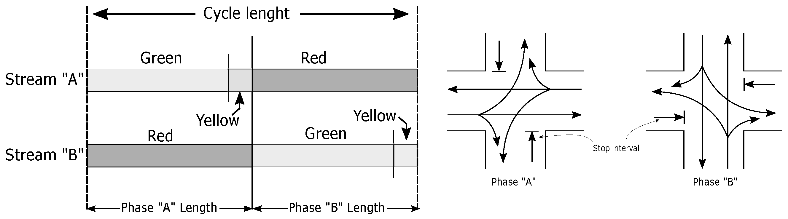
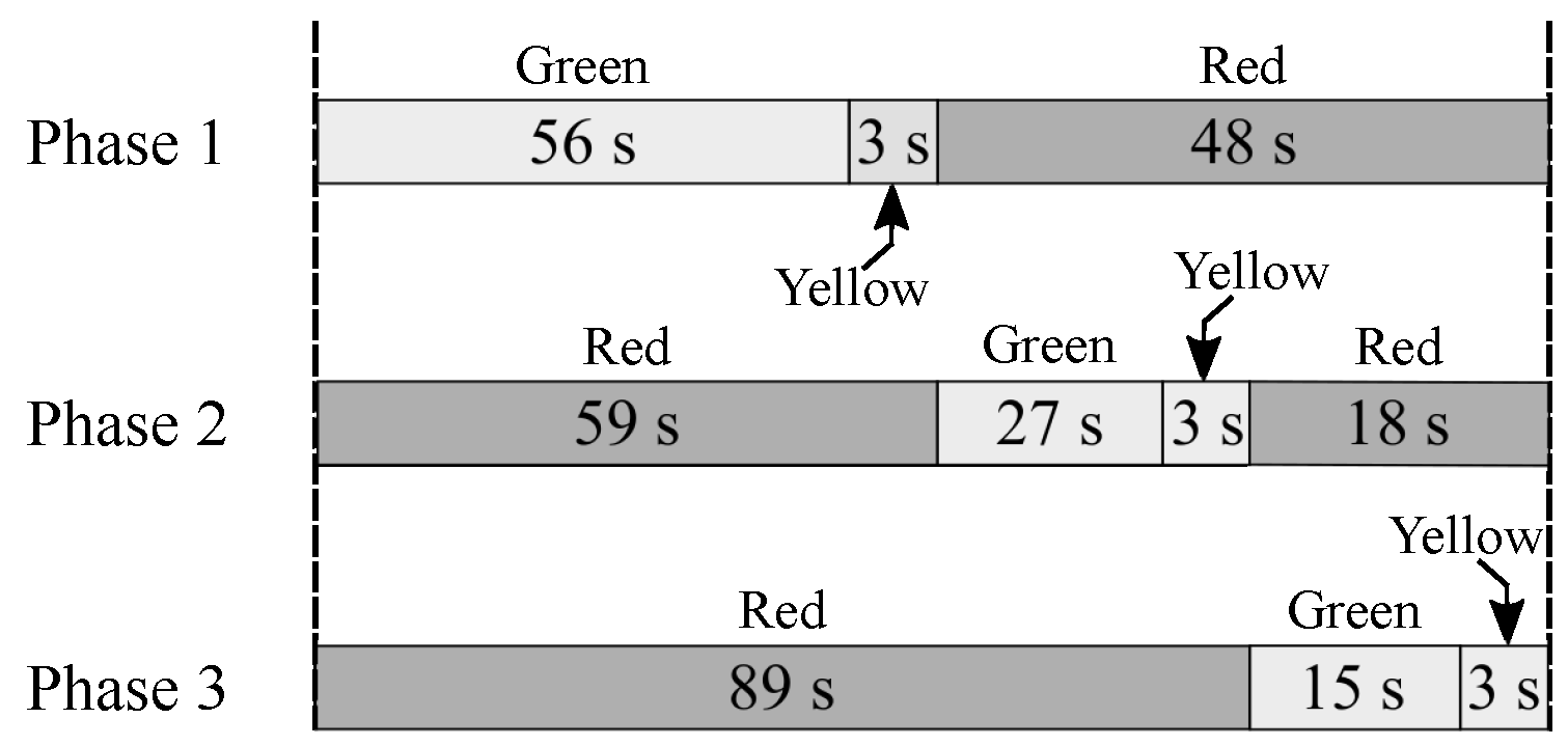
3.1. Traffic Signal Timing
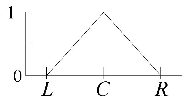
3.2. Fuzzy Logic
4. Proposed Adaptive Traffic Signal Controller Based on Fuzzy Logic
4.1. Fuzzy Inference Description
| Algorithm 1 Fuzzy inference module |
|
4.2. Adaptive Mechanism Description
| Algorithm 2 Adaptive mechanism module. |
| Input: Output: Phases configuration
|
5. Evaluation and Discussion
5.1. Implementation of the Proposed Controller
- 1.
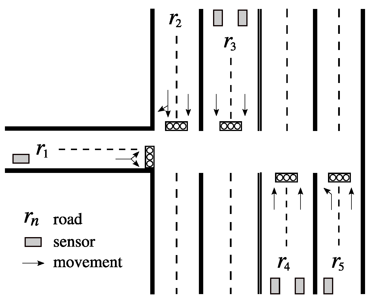
- is a two-lane dual road with west–east and east–west traffic. In addition, has two turning movements: a permitted right turn allowing the incorporation of vehicles to and , and a protected left turn for the incorporation of vehicles to and .
- 2.
- and are two-lane single roads with north–south traffic.
- 3.
- and are two-lane single roads with south–north traffic. Moreover, has a protected left turn to allow the incorporation of vehicles to and .
- 1.
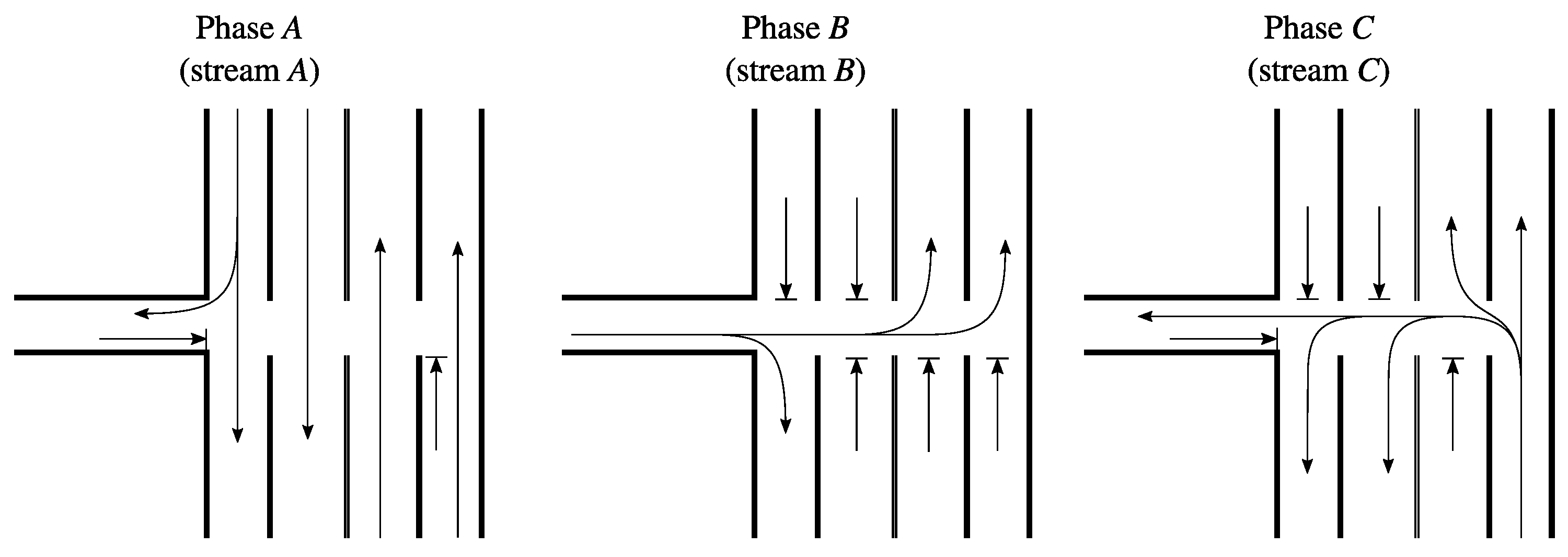
- Stream A is composed by the through movements of , , and , along with the permitted right turn of .
- 2.
- Stream B is composed of the two movements of , a protected left turn and a permitted right turn.
- 3.
- Stream C is composed of both movements of , the protected left turn and the through movement.
- 1.
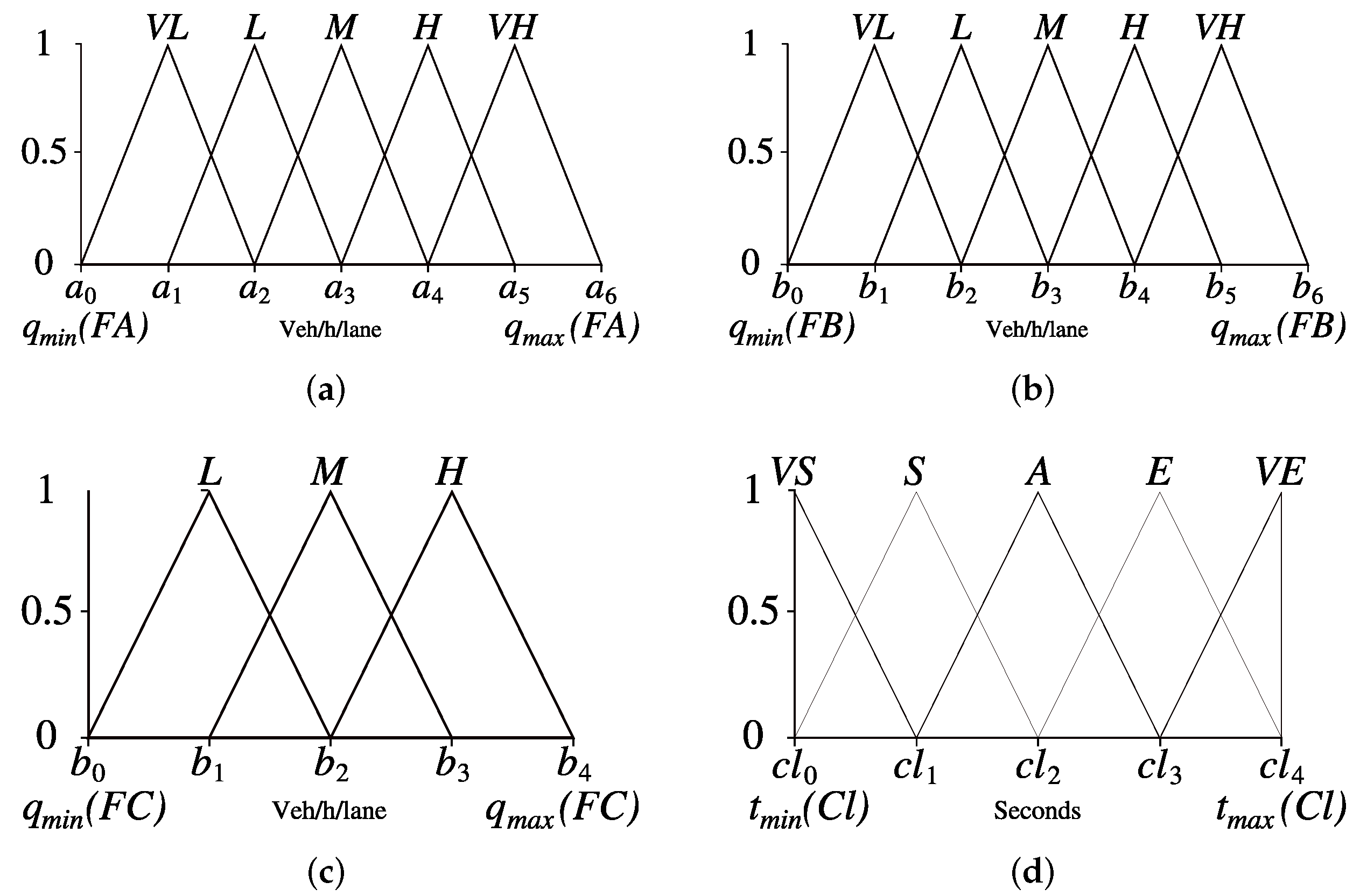
- Flow A () is the variable whose universe of discourse is the traffic flow rate of stream A.
- 2.
- Flow B () is the input related to the flow rate of stream B.
- 3.
- Flow C () is related to the flow rate of stream C.
- 4.
- Cycle length () is the variable whose universe of discourse is the duration of the set of phases in the traffic signal.
- 1.
- Flows A and B are fuzzified through five fuzzy sets: very low ( ), low (L), medium (M), high (H), and very high ().
- 2.
- Since Flow C has the less traffic flow rates, only three membership functions are defined: low (L), medium (M), and high (H).
- 3.
- The cycle length is fuzzified with five functions: very short (), short (S), average (A), extended (E), and very extended ().
5.2. Simulation Model
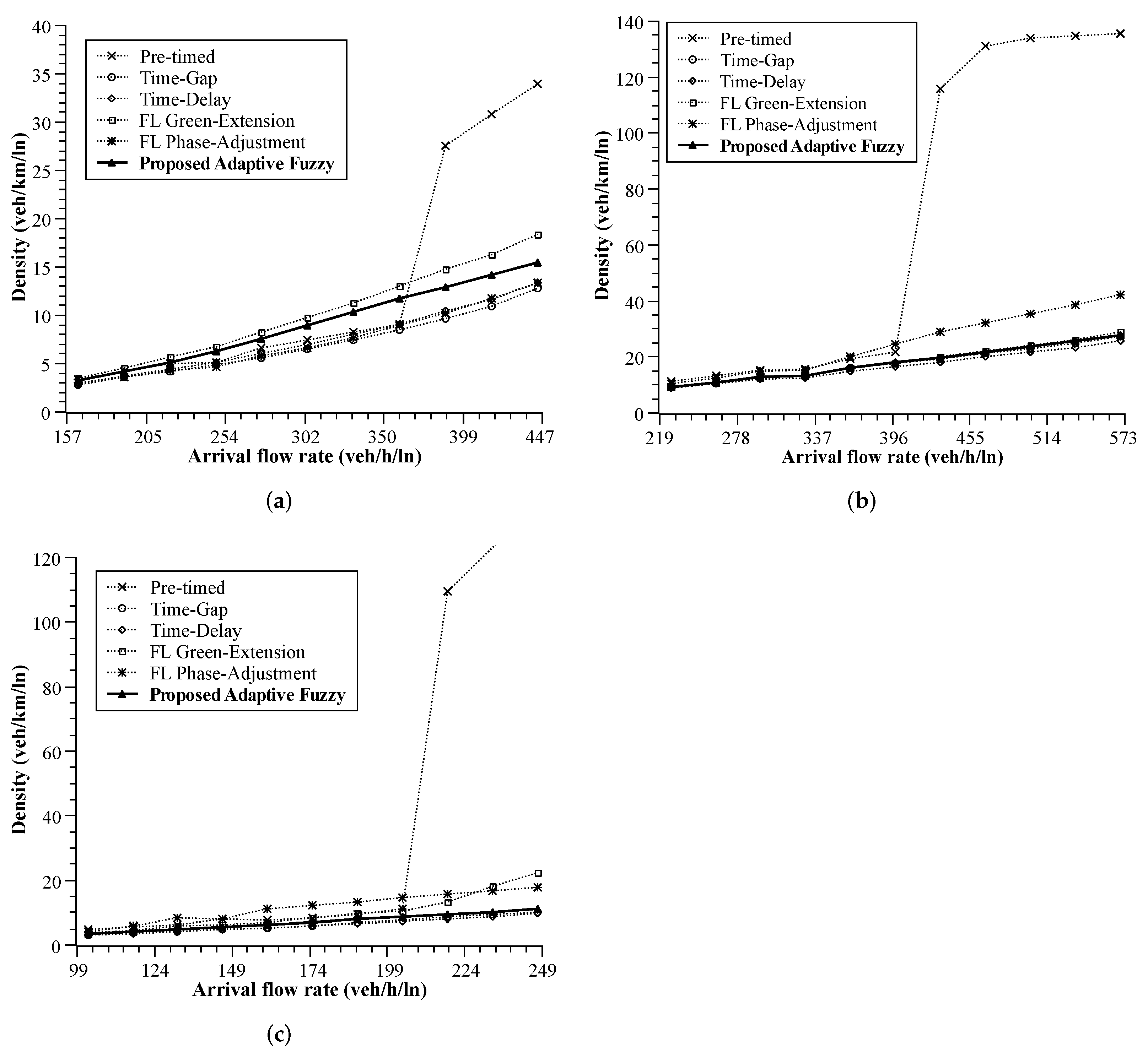
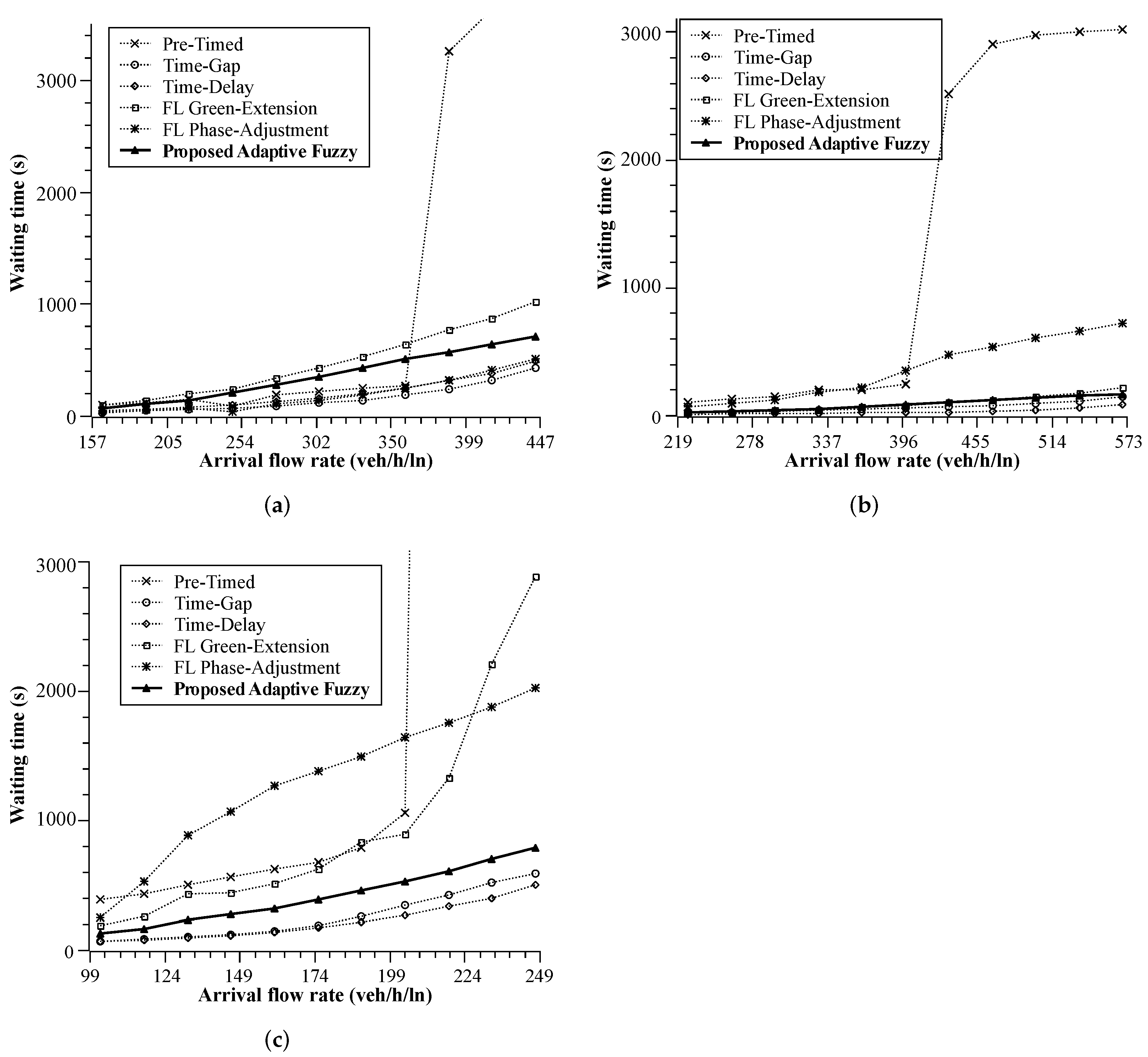
5.3. Comparison against Other Approaches
5.4. Prospective Strengths of Proposal
6. Conclusions
Author Contributions
Funding
Conflicts of Interest
References
- Zapotecatl, J.L.; Rosenblueth, D.A.; Gershenson, C. Deliberative Self-Organizing Traffic Lights with Elementary Cellular Automata. Complexity 2017, 2017, 7691370. [Google Scholar] [CrossRef]
- Krzysztof, M. The Importance of Automatic Traffic Lights time Algorithms to Reduce the Negative Impact of Transport on the Urban Environment. Transp. Res. Procedia 2016, 16, 329–342. [Google Scholar] [CrossRef] [Green Version]
- He, Q.; Kamineni, R.; Zhang, Z. Traffic signal control with partial grade separation for oversaturated conditions. Transp. Res. Part C Emerg. Technol. 2016, 71, 267–283. [Google Scholar] [CrossRef]
- Kutadinata, R.; Moase, W.; Manzie, C.; Zhang, L.; Garoni, T. Enhancing the performance of existing urban traffic light control through extremum-seeking. Transp. Res. Part C Emerg. Technol. 2016, 62, 1–20. [Google Scholar] [CrossRef]
- Grandinetti, P.; de Wit, C.C.; Garin, F. Distributed Optimal Traffic Lights Design for Large-Scale Urban Networks. IEEE Trans. Control Syst. Technol. 2018, 27, 950–963. [Google Scholar] [CrossRef] [Green Version]
- Shirke, C.; Sabar, N.; Chung, E.; Bhaskar, A. Metaheuristic approach for designing robust traffic signal timings to effectively serve varying traffic demand. J. Intell. Transp. Syst. 2022, 26, 343–355. [Google Scholar] [CrossRef]
- Toledo, T.; Balasha, T.; Keblawi, M. Optimization of Actuated Traffic Signal Plans Using a Mesoscopic Traffic Simulation. J. Transp. Eng. Part A Syst. 2020, 146, 04020041. [Google Scholar] [CrossRef]
- Nie, C.; Wei, H.; Shi, J.; Zhang, M. Optimizing actuated traffic signal control using license plate recognition data: Methods for modeling and algorithm development. Transp. Res. Interdiscip. Perspect. 2021, 9, 100319. [Google Scholar] [CrossRef]
- Li, L.; Huang, W.; Lo, H.K. Adaptive coordinated traffic control for stochastic demand. Transp. Res. Part C Emerg. Technol. 2018, 88, 31–51. [Google Scholar] [CrossRef]
- Gershenson, C. Self-Organizing Traffic Lights. Complex Syst. 2005, 16, 29–53. [Google Scholar]
- Gershenson, C.; Rosenblueth, D.A. Self-organizing traffic lights at multiple-street intersections. Int. J. Sci. Res. Publ. 2012, 17, 23–39. [Google Scholar] [CrossRef] [Green Version]
- Ge, Y. A Two-Stage Fuzzy Logic Control Method of Traffic Signal Based on Traffic Urgency Degree. Model. Simul. Eng. 2014, 2014, 694185. [Google Scholar] [CrossRef] [Green Version]
- Aslani, M.; Mesgari, M.S.; Wiering, M. Adaptive traffic signal control with actor-critic methods in a real-world traffic network with different traffic disruption events. Transp. Res. Part C Emerg. Technol. 2017, 85, 732–752. [Google Scholar] [CrossRef] [Green Version]
- Jin, J.; Ma, X. A multi-objective multi-agent framework for traffic light control. In Proceedings of the 2017 11th Asian Control Conference (ASCC), Gold Coast, Australia, 17–20 December 2017; pp. 1199–1204. [Google Scholar]
- Xu, Y.; Xi, Y.; Li, D.; Zhou, Z. Traffic Signal Control based on Markov Decision Process. IFAC-PapersOnLine 2016, 49, 67–72. [Google Scholar] [CrossRef]
- Castro, G.B.; Hirakawa, A.R.; Martini, J.S. Adaptive traffic signal control based on bio-neural network. Procedia Comput. Sci. 2017, 109, 1182–1187. [Google Scholar] [CrossRef]
- Jiang, L.; Li, Y.; Liu, Y.; Chen, C. Traffic signal light control model based on evolutionary programming algorithm optimization BP neural network. In Proceedings of the 2017 7th IEEE International Conference on Electronics Information and Emergency Communication (ICEIEC), Macau, China, 21–23 July 2017; pp. 564–567. [Google Scholar] [CrossRef]
- Kaur, T.; Agrawal, S. Adaptive traffic lights based on hybrid of neural network and genetic algorithm for reduced traffic congestion. In Proceedings of the 2014 Recent Advances in Engineering and Computational Sciences (RAECS), Chandigarh, India, 6–8 March 2014; pp. 1–5. [Google Scholar] [CrossRef]
- Ge, H.; Song, Y.; Wu, C.; Ren, J.; Tan, G. Cooperative Deep Q-Learning With Q-Value Transfer for Multi-Intersection Signal Control. IEEE Access 2019, 7, 40797–40809. [Google Scholar] [CrossRef]
- Liang, X.; Du, X.; Wang, G.; Han, Z. A Deep Reinforcement Learning Network for Traffic Light Cycle Control. IEEE Trans. Veh. Technol. 2019, 68, 1243–1253. [Google Scholar] [CrossRef] [Green Version]
- Gu, J.; Fang, Y.; Sheng, Z.; Wen, P. Double Deep Q-Network with a Dual-Agent for Traffic Signal Control. Appl. Sci. 2020, 10, 1622. [Google Scholar] [CrossRef] [Green Version]
- Park, S.; Han, E.; Park, S.; Jeong, H.; Yun, I. Deep Q-network-based traffic signal control models. PLoS ONE 2021, 16, e256405. [Google Scholar] [CrossRef]
- Zaied, A.N.H.; Othman, W.A. Development of a fuzzy logic traffic system for isolated signalized intersections in the State of Kuwait. Expert Syst. Appl. 2011, 38, 9434–9441. [Google Scholar] [CrossRef]
- Balaji, P.; Srinivasan, D. Type-2 fuzzy logic based urban traffic management. Eng. Appl. Artif. Intell. 2011, 24, 12–22. [Google Scholar] [CrossRef]
- Aksaç, A.; Uzun, E.; Özyer, T.A. A real time traffic simulator utilizing an adaptive fuzzy inference mechanism by tuning fuzzy parameters. Appl. Intell. 2012, 32, 698–720. [Google Scholar] [CrossRef]
- Chiou, Y.C.; Huang, Y.F. Stepwise genetic fuzzy logic signal control under mixed traffic conditions. J. Adv. Transp. 2013, 47, 43–60. [Google Scholar] [CrossRef]
- Adam, I.; Wahab, A.; Yaakop, M.; Salam, A.A.; Zaharudin, Z. Adaptive fuzzy logic traffic light management system. In Proceedings of the 2014 4th International Conference on Engineering Technology and Technopreneuship (ICE2T), Kuala Lumpur, Malaysia, 27–29 August 2014; pp. 340–343. [Google Scholar] [CrossRef]
- Bi, Y.; Srinivasan, D.; Lu, X.; Sun, Z.; Zeng, W. Type-2 fuzzy multi-intersection traffic signal control with differential evolution optimization. Expert Syst. Appl. 2014, 41, 7338–7349. [Google Scholar] [CrossRef]
- Collotta, M.; Bello, L.L.; Pau, G. A novel approach for dynamic traffic lights management based on Wireless Sensor Networks and multiple fuzzy logic controllers. Expert Syst. Appl. 2015, 42, 5403–5415. [Google Scholar] [CrossRef]
- Ibrahim, L.M.; Aldabbagh, M.A. Adaptive Fuzzy Control to Design and Implementation of Traffic Simulation System. Int. J. Sci. Res. Publ. 2016, 14, 228–246. [Google Scholar]
- Khooban, M.H.; Vafamand, N.; Liaghat, A.; Dragicevic, T. An optimal general type-2 fuzzy controller for Urban Traffic Network. ISA Trans. 2017, 66, 335–343. [Google Scholar] [CrossRef]
- Mahmood, T.; Ali, M.E.M.; Durdu, A. A two Stage Fuzzy Logic Adaptive Traffic Signal Control for an Isolated Intersection Based on Real Data using SUMO Simulator. Int. J. Trend Sci. Res. Dev. 2019, 3, 656–659. [Google Scholar] [CrossRef]
- Dewasme, L.; Jiang, T.; Wang, Z.; Chen, F. Urban Traffic Signals Timing at Four-Phase Signalized Intersection Based on Optimized Two-Stage Fuzzy Control Scheme. Math. Probl. Eng. 2021, 2021, 6693562. [Google Scholar] [CrossRef]
- Ali, M.E.M.; Durdu, A.; Celtek, S.A.; Yilmaz, A. An Adaptive Method for Traffic Signal Control Based on Fuzzy Logic with Webster and Modified Webster Formula Using SUMO Traffic Simulator. IEEE Access 2021, 9, 102985–102997. [Google Scholar] [CrossRef]
- Araghi, S.; Khosravi, A.; Creighton, D. A review on computational intelligence methods for controlling traffic signal timing. Expert Syst. Appl. 2015, 42, 1538–1550. [Google Scholar] [CrossRef]
- Gregurić, M.; Vujić, M.; Alexopoulos, C.; Miletić, M. Application of Deep Reinforcement Learning in Traffic Signal Control: An Overview and Impact of Open Traffic Data. Appl. Sci. 2020, 10, 4011. [Google Scholar] [CrossRef]
- Rasheed, F.; Yau, K.L.A.; Noor, R.M.; Wu, C.; Low, Y.C. Deep Reinforcement Learning for Traffic Signal Control: A Review. IEEE Access 2020, 8, 208016–208044. [Google Scholar] [CrossRef]
- Lawry, J. Modelling and Reasoning with Vague Concepts; Studies in Computational Intelligence; Springer: New York, NY, USA, 2006. [Google Scholar]
- Al-Sobky, A.S.A.; Mousa, R.M. Traffic density determination and its applications using smartphone. Alex. Eng. J. 2016, 55, 513–523. [Google Scholar] [CrossRef] [Green Version]
- Wu, A.; Yang, X. Real-time Queue Length Estimation of Signalized Intersections Based on RFID Data. Procedia-Soc. Behav. Sci. 2013, 96, 1477–1484. [Google Scholar] [CrossRef] [Green Version]
- Asmaa, O.; Mokhtar, K.; Abdelaziz, O. Road traffic density estimation using microscopic and macroscopic parameters. Image Vis. Comput. 2013, 31, 887–894. [Google Scholar] [CrossRef]
- Webster, F. Traffic Signal Settings; Road Research Technical Paper; H.M. Stationery Office: Richmond, UK, 1958. [Google Scholar]
- Oertel, R.; Wagner, P. Delay-time actuated traffic signal control for an isolated intersection. In Proceedings of the Transportation Research Board 2011 (90th Annual Meeting), Washington, DC, USA, 23–27 January 2011. Number EPFL-CONF-181089. [Google Scholar]
- Erdmann, J.; Oertel, R.; Wagner, P. VITAL: A Simulation-Based Assessment of New Traffic Light Controls. In Proceedings of the 2015 IEEE 18th International Conference on Intelligent Transportation Systems, Gran Canaria, Spain, 15–18 September 2015; pp. 25–29. [Google Scholar]
- Zhou, Z.; Cai, M. Intersection signal control multi-objective optimization based on genetic algorithm. J. Traffic Transp. Eng. (English Ed.) 2014, 1, 153–158. [Google Scholar] [CrossRef] [Green Version]
- Foulaadvand, M.; Sadjadi, Z.; Reza Shaebani, M. Optimized traffic flow at a single intersection: Traffic responsive signalization. J. Phys. A Math. Gen. 2004, 37, 561. [Google Scholar] [CrossRef] [Green Version]
- Wiering, M.; Vreeken, J.; van Veenen, J.; Koopman, A. Simulation and optimization of traffic in a city. In Proceedings of the IEEE Intelligent Vehicles Symposium, Parma, Italy, 14–17 June 2004; pp. 453–458. [Google Scholar] [CrossRef] [Green Version]
- Mirchandani, P.; Head, L. A real-time traffic signal control system: Architecture, algorithms, and analysis. Transp. Res. Part C Emerg. Technol. 2001, 9, 415–432. [Google Scholar] [CrossRef]
- Vincent, R.A.; Young, C.P. Self-Optimizing Traffic Signal Control Using Microprocessors: The TRRL MOVA Strategy For Isolated Intersections. In Proceedings of the 2nd International Conference on Road Traffic Control, London, UK, 15–18 April 1986; pp. 102–105. [Google Scholar]
- Little, J.; Kelson, M.; Gartner, N. MAXBAND: A program for setting signals on arteries and triangular networks. In Transport of Washington DC Transport Research Record (795); National Research Council: Washington, DC, USA, 1981. [Google Scholar]
- Vincent, R.; Peirce, J. ‘MOVA’: Traffic Responsive, Self-Optimising Signal Control for Isolated Intersections; Technical Report; Traffic Management Division, Traffic Group, Transport and Road Research Laboratory Crowthorne: Berkshire, UK, 1988. [Google Scholar]
- Peter, K.; Rodegerdts, L.; Lee, K.; Quayle, S.; Beaird, S.; Braud, C.; Bonneson, J.; Tarnoff, P.; Urbanik, T. Traffic Signal Timing Manual; Technical Report; Federal Highway Administration: Washington, DC, USA, 2008.
- Zheng, X.; Recker, W.; Chu, L. Optimization of Control Parameters for Adaptive Traffic-Actuated Signal Control. J. Intell. Transp. Syst. 2010, 14, 95–108. [Google Scholar] [CrossRef]
- Zheng, X.; Recker, W. An adaptive control algorithm for traffic-actuated signals. Transp. Res. Part C Emerg. Technol. 2013, 30, 93–115. [Google Scholar] [CrossRef]
- Jeong, J.; Shen, Y.; Oh, T.; Céspedes, S.; Benamar, N.; Wetterwald, M.; Härri, J. A comprehensive survey on vehicular networks for smart roads: A focus on IP-based approaches. Veh. Commun. 2021, 29, 100334. [Google Scholar] [CrossRef]
- Jiang, L.; Molnár, T.G.; Orosz, G. On the deployment of V2X roadside units for traffic prediction. Transp. Res. Part C Emerg. Technol. 2021, 129, 103238. [Google Scholar] [CrossRef]
- Katsaros, K.; Kernchen, R.; Dianati, M.; Rieck, D. Performance study of a Green Light Optimized Speed Advisory (GLOSA) application using an integrated cooperative ITS simulation platform. In Proceedings of the 2011 7th International Wireless Communications and Mobile Computing Conference, Istanbul, Turkey, 4–8 July 2011; pp. 918–923. [Google Scholar] [CrossRef]
- Shiri, M.S.; Maleki, H.R. Maximum Green Time Settings for Traffic-Actuated Signal Control at Isolated Intersections Using Fuzzy Logic. Int. J. Fuzzy Syst. 2017, 19, 247–256. [Google Scholar] [CrossRef]
- Yin, B.; Menendez, M. A Reinforcement Learning Method for Traffic Signal Control at an Isolated Intersection with Pedestrian Flows. In Proceedings of the CICTP 2019: Transportation in China—Connecting the World Transportation in China—Proceedings of the 19th COTA International Conference of Transportation Professionals, Nanjing, China, 6–8 July 2019; pp. 3123–3135. [Google Scholar] [CrossRef]
- Kővári, B.; Szőke, L.; Bécsi, T.; Aradi, S.; Gáspár, P. Traffic Signal Control via Reinforcement Learning for Reducing Global Vehicle Emission. Sustainability 2021, 13, 11254. [Google Scholar] [CrossRef]
- Prasetiyo, E.E.; Wahyunggoro, O.; Solistyo, S. Design and simulation of adaptive traffic light controller using fuzzy logic control sugeno method. Int. J. Sci. Res. Publ. 2015, 5, 1–6. [Google Scholar]
- Wolput, B.; Christofa, E.; Tampère, C.M.J. Optimal Cycle-Length Formulas for Intersections With or Without Transit Signal Priority. Transp. Res. Rec. 2016, 2558, 78–91. [Google Scholar] [CrossRef]
- Zakariya, A.Y.; Rabia, S.I. Estimating the minimum delay optimal cycle length based on a time-dependent delay formula. Alex. Eng. J. 2016, 55, 2509–2514. [Google Scholar] [CrossRef] [Green Version]
- Krajzewicz, D.; Erdmann, J.; Behrisch, M.; Bieker, L. Recent Development and Applications of SUMO - Simulation of Urban MObility. Int. J. Adv. Syst. Meas. 2012, 5, 128–138. [Google Scholar]
- Novák, V.; Mockor, J.; Perfilieva, I. Mathematical Principles of Fuzzy Logic; Kluwer International Series in Engineering and Computing Science; Kluwer: Boston, MA, USA, 1999. [Google Scholar]
- Zadeh, L.A. Fuzzy Sets. Inf. Control 1965, 8, 338–353. [Google Scholar] [CrossRef] [Green Version]
- Sugeno, M. An introductory survey of fuzzy control. Inf. Sci. 1985, 36, 59–83. [Google Scholar] [CrossRef]
- Lee, C.C. Fuzzy logic in control systems: Fuzzy logic controller. Parts I and II. IEEE Trans. Syst. Man Cybern. 1990, 20, 404–435. [Google Scholar] [CrossRef] [Green Version]
- Ross, T.J. Properties of membership functions fuzzification and defuzzification. In Fuzzy Logic with Engineering Applications; McGraw Hill: New York, NY, USA, 1995. [Google Scholar]
- Mamdani, E.H.; Assilian, S. An experiment in linguistic synthesis with a fuzzy logic controller. Int. J. Man-Mach. Stud. 1975, 7, 1–13. [Google Scholar] [CrossRef]
- Mamdani, E.H. Application of Fuzzy Logic to Approximate Reasoning Using Linguistic Synthesis. IEEE Trans. Comput. 1977, 26, 1182–1191. [Google Scholar] [CrossRef]
- Board, T.R. Highway Capacity Manual 6th Edition: A Guide for Multimodal Mobility Analysis; The National Academies Press: Washington, DC, USA, 2016. [Google Scholar] [CrossRef]
- Wegener, A.; Piórkowski, M.; Raya, M.; Hellbrück, H.; Fischer, S.; Hubaux, J.P. TraCI: An Interface for Coupling Road Traffic and Network Simulators. In Proceedings of 11th Communications and Networking Simulation Symposium CNS ’08, Ottawa, ON, Canada, 14–17 April 2008; Association for Computing Machinery: New York, NY, USA, 2008; pp. 155–163. [Google Scholar] [CrossRef]
- Wegener, A.; Hellbruck, H.; Wewetzer, C.; Lubke, A. VANET Simulation Environment with Feedback Loop and its Application to Traffic Light Assistance. In Proceedings of the 2008 IEEE Globecom Workshops, New Orleans, LA, USA, 30 November–1 December 2008; pp. 1–7. [Google Scholar] [CrossRef]
- Xiaorui, W.; Hongxu, Y. A Lane Change Model with the Consideration of Car Following Behavior. Procedia-Soc. Behav. Sci. 2013, 96, 2354–2361. [Google Scholar] [CrossRef] [Green Version]
- Krauss, S. Microscopic Modeling of Traffic Flow: Investigation of Collision Free Vehicle Dynamics. Ph.D. Thesis, University of Cologne, Cologne, Germany, 1998. [Google Scholar]
- Dalaff, C.; Ebendt, R.; Erdmann, J.; Gurczik, G.; Touko, L.C. Benchmarking SUMO generated traffic simulation results based on GEH Statistic. In Proceedings of the 1st SUMO User Conference, Berlin, Germany, 15–17 May 2013; p. 54. [Google Scholar]
- Traffic Lights That Respond to Traffic. SUMO Documentation. Available online: https://sumo.dlr.de/docs/Simulation/Traffic_Lights.html (accessed on 13 June 2022).
- Krajzewicz, D.; Brockfeld, E.; Mikat, J.; Ringel, J.; Feld, C.; Tuchscheerer, W.; Wagner, P.; Woesler, R. Simulation of modern Traffic Lights Control Systems using the open source Traffic Simulation SUMO. In Proceedings of the 3rd Industrial Simulation Conference, Berlin, Germany, 9–11 June 2005; pp. 299–302. [Google Scholar]
- Goldmann, K.; Sieg, G. Economic implications of phantom traffic jams: Evidence from traffic experiments. Transp. Lett. 2020, 12, 386–390. [Google Scholar] [CrossRef]
- VITAL Project. Available online: www.projekt-vital.de (accessed on 13 June 2022).
- MAVEN. Deliverable 3.3: Cooperative Manoeuvre and Trajectory Planning Algorithms; Technical Report, Grant Agreement No. 690727; Managing Automated Vehicles Enhances Network: Amersfoort, The Netherlands, 2020; Available online: http://adas.cvc.uab.es/maven/enigma-portfolio/d3-3-cooperative-manoeuvre-and-trajectory-planning-algorithms/ (accessed on 13 June 2022).
- Managing Automated Vehicles Enhances Network (MAVEN). Available online: http://maven-its.eu (accessed on 13 June 2022).


| Rule | Input | Output | ||
|---|---|---|---|---|
| Flow A | Flow B | Flow C | Cycle Length | |
| 1 | Very Low | Very Low | Low | Very Short |
| 2 | Low | Very Low | Low | Very Short |
| 3 | Medium | Very Low | Low | Short |
| 4 | High | Very Low | Low | Average |
| 5 | Very High | Very Low | Low | Average |
| 6 | Very Low | Low | Low | Very Short |
| 7 | Low | Low | Low | Very Short |
| 8 | Medium | Low | Low | Short |
| 9 | High | Low | Low | Average |
| … | … | … | … | … |
| 75 | Medium | Medium | Medium | Average |
| Roads | |||||
|---|---|---|---|---|---|
| Traffic volume (veh/day) | 4765 | 5393 | 8652 | 9450 | 4664 |
| Avg. travel speed (km/h) | 32.20 | 28.30 | 42.30 | 57.90 | 26.40 |
| Mean flow rate (veh/h) | 451 | 329 | 554 | 770 | 226 |
| Roads | |||||||
|---|---|---|---|---|---|---|---|
| Hour | Avg. | ||||||
| Flow rate (Veh/h) | 7:00–8:00 | 417 | 221 | 543 | 686 | 201 | 422 |
| 8:00–9:00 | 386 | 252 | 502 | 759 | 212 | 414 | |
| 9:00–10:00 | 347 | 157 | 450 | 644 | 190 | 358 | |
| 10:00–11:00 | 344 | 209 | 445 | 602 | 175 | 355 | |
| 11:00–12:00 | 341 | 207 | 475 | 547 | 172 | 348 | |
| 12:00–13:00 | 323 | 220 | 517 | 561 | 197 | 364 | |
| 13:00–14:00 | 312 | 234 | 597 | 613 | 226 | 396 | |
| 14:00–15:00 | 324 | 238 | 608 | 537 | 233 | 388 | |
| 15:00–16:00 | 356 | 234 | 543 | 597 | 555 | 457 | |
| 16:00–17:00 | 321 | 223 | 513 | 605 | 202 | 373 | |
| 17:00–18:00 | 347 | 219 | 494 | 641 | 194 | 379 | |
| 18:00–19:00 | 359 | 221 | 550 | 615 | 198 | 389 | |
| 19:00–20:00 | 417 | 232 | 557 | 546 | 222 | 395 | |
| 20:00–21:00 | 255 | 226 | 528 | 409 | 208 | 325 | |
| Destination | ||||||
|---|---|---|---|---|---|---|
| Origin | — | 3.64% | 6.16% | 16.81% | 73.38% | |
| 18.23% | 81.77% | — | — | — | ||
| — | — | 100% | — | — | ||
| — | — | — | 100% | — | ||
| 74.62% | 11.19% | 13.43% | — | 0.74% | ||
Publisher’s Note: MDPI stays neutral with regard to jurisdictional claims in published maps and institutional affiliations. |
© 2022 by the authors. Licensee MDPI, Basel, Switzerland. This article is an open access article distributed under the terms and conditions of the Creative Commons Attribution (CC BY) license (https://creativecommons.org/licenses/by/4.0/).
Share and Cite
Madrigal Arteaga, V.M.; Pérez Cruz, J.R.; Hurtado-Beltrán, A.; Trumpold, J. Efficient Intersection Management Based on an Adaptive Fuzzy-Logic Traffic Signal. Appl. Sci. 2022, 12, 6024. https://doi.org/10.3390/app12126024
Madrigal Arteaga VM, Pérez Cruz JR, Hurtado-Beltrán A, Trumpold J. Efficient Intersection Management Based on an Adaptive Fuzzy-Logic Traffic Signal. Applied Sciences. 2022; 12(12):6024. https://doi.org/10.3390/app12126024
Chicago/Turabian StyleMadrigal Arteaga, Victor Manuel, José Roberto Pérez Cruz, Antonio Hurtado-Beltrán, and Jan Trumpold. 2022. "Efficient Intersection Management Based on an Adaptive Fuzzy-Logic Traffic Signal" Applied Sciences 12, no. 12: 6024. https://doi.org/10.3390/app12126024
APA StyleMadrigal Arteaga, V. M., Pérez Cruz, J. R., Hurtado-Beltrán, A., & Trumpold, J. (2022). Efficient Intersection Management Based on an Adaptive Fuzzy-Logic Traffic Signal. Applied Sciences, 12(12), 6024. https://doi.org/10.3390/app12126024