
A Novel Energy-Saving Route Planning Algorithm for Marine Vehicles


1
Mathematics and Computer Science College, Guangdong Ocean University, Zhanjiang 524000, China
2
Maritime College, Guangdong Ocean University, Zhanjiang 524000, China
3
Technical Research Center for Ship Intelligence and Safety Engineering of Guangdong Province, Zhanjiang 524000, China
4
School of Navigation, Guangzhou Maritime University, Guangzhou 510725, China
*
Author to whom correspondence should be addressed.
Appl. Sci. 2022, 12(12), 5971; https://doi.org/10.3390/app12125971
Submission received: 21 April 2022
/
Revised: 31 May 2022
/
Accepted: 7 June 2022
/
Published: 11 June 2022
(This article belongs to the Special Issue Maritime Transportation System and Traffic Engineering)
Abstract
:Recently, the ship energy consumption issue has been in the spotlight. Meanwhile, new conventions and standards of ship energy conservation as well as ship emission reduction have been continuously introduced by the International Maritime Organization and governments around the world. Energy conservation is a crucial factor in ship route planning. This paper proposes an improved ant colony algorithm that can handle a complicated ocean current environment and find an optimal energy-saving path. Firstly, this paper focuses on both the path length and energy consumption. To reduce energy consumption, a comprehensive energy cost function is introduced by a conventional ant colony algorithm. In addition, this paper analyzes the influence of the ocean current speed and setting on a marine vehicle and establishes an improved ant colony algorithm model based on the influence of the ocean current. Finally, simulation tests are carried out in Lianyungang and its surrounding areas to test the energy consumption performance of the improved ant colony algorithm. The simulation result shows that the improved ant colony algorithm can significantly reduce the energy consumption by 3.326% compared with the traditional algorithm.
1. Introduction
Most marine vehicles use fuel as their power source, and their voyage is limited by the fuel they carry [1]. Efficient employ of limited energy for long-time and long-distance voyages is the major challenge facing marine vehicles at present [2,3]. To settle this problem, scholars have proposed various methods to reduce the energy consumption of marine vehicles. Among these methods, the route planning method is not only conducive to reducing the influence of complex ocean conditions on the power consumption of ships, but it also improves the safety of ships. Therefore, the ship route planning method has received attention from many researchers.
In this aspect, the route planning of marine vehicles could be global or local. For global route planning, ships would identify all spaces with obstacles in the given chart in advance, and then to choose an energy-saving route without obstacles. In comparison, local route planning utilizes the obstacle avoidance algorithm to achieve the same result [4,5,6]. In global path planning, scholars have proposed many algorithms for optimal ship route planning tasks. The literature [7,8,9,10,11] has employed a genetic algorithm to search the ship’s route. However, the genetic algorithm is a unstable and time-consuming algorithm. The literature [12,13,14] has employed a particle swarm optimization algorithm to achieve ship functions of obstacle avoidance and trajectory optimization. This algorithm is simple, with good robustness, and has a fast early-stage convergence speed, but the convergence speed becomes slow in the later stage of the search. Shen et al. [15] addressed the wolf pack algorithm to study the navigation and route planning of ships. This algorithm applies the wolf pack update mechanism to optimize the complex search space. Although the algorithm has good convergence, global optimization, and strong robustness, it is relatively complicated owing to more parameters to be set.
Among recent research of route planning based on energy-saving, Qu [16] proposed a constrained sampling A star (CSA*) algorithm for enhancing search effects. Meanwhile, adaptive quantum-behaved particle swarm optimization (AQPSO) is integrated with the CSA*, which could cut down the energy expenditure in case of currents influence. Dong [17] proposed a novel double ant colony algorithm (NDACA) on the basis of dynamic feedback. The ant colony is grouped as exploratory and optimized ants according to the pheromone. A closed-cycle feedback tactic is applied to constantly adjust the number of ants in every colony, which could improve the resolution quality and speed up the convergence. NDACA could plan a route with less energy consumption and also take the influence of marine environment factors into account. Pan [18] proposed a new genetic-ant compound algorithm. As a novel optimal integrated strategy, this algorithm increases the efficiency of integration. Meanwhile, taking into account the energy consumption under the currents influence, it sets up the merit function on the basis of minimized energy consumption.
Compared with the above algorithms, the ant colony algorithm has the advantages of low requirements on initial route selection and strong robustness. It is vital that the ant colony algorithm has relatively fewer parameters and does not require manual adjustment, which is more suitable for ship route planning in complex marine environments [19]. In addition, the ant colony algorithm has great advantages in solving the TSP (traveling salesman problem) of marine vehicles [20,21,22]. Scholars have proposed many improved ant colony algorithms and applied them to the route optimization of marine vehicles [23]. Cao [24] proposed a path planning algorithm considering ocean currents, which combines artificial potential field method and ant colony algorithm. It avoids the local extremum problem of artificial potential field method and improves the performance of ant colony algorithm. Di [25] used an ant colony algorithm based on ocean current and path length, which modified the transition probability formula in the simulated ocean current environment and realized the optimal route planning of marine vehicles with low energy consumption and short sailing distance.
Although the ant colony algorithm has certain advantages in processing energy-saving problems, the above two ant colony-based algorithm models hardly meet the real ocean environments, due to that those models do not support the changing ocean current environments. In this paper, a route optimization method based on an improved ant colony algorithm is proposed, which meets the requirement of energy-saving and long-term use of marine vehicles in complex marine environments. Compared with other methods, our route optimization design method takes into account changes in the velocity and direction of ocean current, as well as the effect of route length on energy consumption, so that it can plan a path that consumes the least energy. The paper is structured as follows: Section 2 presents the problem description. Section 3 presents the method. Section 4 conducts experimental simulations. Finally, the conclusion of this paper is given.
2. Formulation of the Energy-Saving Problem
2.1. Optimization Objective
Route planning technology is one of the core issues in the field of marine vehicles. It aims to find an optimal or suboptimal route from the initial state to the target state in the marine environment, and the optimal route here takes the distance as the evaluating indicator. Route planning mainly includes two parts: one is to build the environment model, and the other is to search for the optimal route.
Energy-saving of ships is among the key factors of route planning. Energy consumption is particularly crucial in the route planning of marine vehicles. Especially, when the route is on a large-scale marine environment, the problem of energy consumption becomes prominent. The main purpose of this paper is to study the optimal route planning of the ship’s energy consumption, taking accounting into ocean current. Therefore, the energy consumption model of the ship in the working environment is its crucial component.
The environment model is an abstract description of the marine space that the ship is in. Building the environment model is a process that describes the realistic environment that the ship is in as a proper abstract model by utilizing a set of rules, which is performed before the ship implements the route planning algorithm. Route search is a process that searches for an eligible and feasible route from the environment model. By building the ocean current model, this paper utilized the improved ant colony algorithm to find the route that has the lowest energy consumption of ocean current.
2.2. Ocean Current Model
This paper built a two-dimensional hydrodynamic numerical model to calculate the velocity and setting of ocean current. The incompressible Reynolds-averaged Navier–Stokes equation is solved by the finite volume method. Boussinesq approximation and assumption of shallow water and hydrostatic pressure are considered [26]. The governing equations are as follows.
where t is the time. x and y are Cartesian coordinates. u and v are the average velocity components in the x and y directions, respectively. is the total water depth. is the source–sink term. is the water surface elevation. is the Coriolis force parameter. is the acceleration of gravity. is the actual water density. . and are the wind shear stress components on the water surface. and are the shear stress components of the bed. is the air atmospheric pressure. and are the velocity components of the source. and are the horizontal eddy viscous stress forces.
2.3. Energy Consumption Model
Taking into account the influencing factors of the current on the ship’s navigation, the route planning algorithm is improved by addressing the energy consumption of the ocean current. Firstly, the current distribution chart is rasterized. The hydrodynamic model of ocean currents takes into account the time-varying properties of ocean currents and simulates the changes of ocean currents. Since the ocean current varies slowly with time, for the sake of simplicity, the interval of time unit of the ocean current variation is set as 1 h, which is the constant current during this period. In addition, the grid method is applied to discretize the ocean current to improve the computational efficiency of route planning, as shown in Figure 1.
Combined with the advantages of the grid method environment model, the ocean current information is rasterized to improve the efficiency of the search algorithm. During the modeling process, the number of rows and columns can be determined by selecting certain interval of sea area and grid precision, and the calculation formula is as follows.
where and are the upper boundary. and are the lower boundary. is the grid precision. We choose 0.01 × 0.01 grid precision to build the model.
During the voyage, when in different headings, the ship has various water-facing areas. The water-facing area is decomposed into x and y directions.
where L, B, and d are the ship’s length, breadth, and draft, respectively. is the angle between the motion direction and the -axis. is the projected area in the direction and is the projected area in the direction.
Energy consumption depends on frontal areas in the x and y directions.
where is the seawater resistance coefficient. is the component of the current in . is the component of the current in . is the speed of the ship. is the energy consumed by the ship in the direction and is the energy consumed by the ship in the direction. is the total energy consumed by the ship in the course. is the time that the ship traveled in the course.
As the ship travels from to , the energy cost of the current is , and the required energy as follows.
is the ship’s sailing time from to . The ship’s speed, current setting, and magnitude are assumed to be constant in the grid. When the current speed of the and axis is higher than the ship speed, the ship speed is 0 and there is no energy consumption. Then, the energy and total energy consumption are as follows.
3. Methods
The ant colony algorithm, proposed by the Italian scholar Dorigo M et al. [27] in 1996, can simulate ants’ foraging behavior. It was used firstly to solve the traveling salesman problem.
Ants leave pheromones wherever they go, which is the foundation of the ant colony algorithm. All paths taken by the ant colony from the ant nest to the food are the solution spaces of the problem, and the shortest path in the solution space retains the most pheromones. When new ants looking for food are faced with different paths, the path with higher pheromone level is often preferred. Eventually, under the positive feedback, the entire ant colony will focus on the shortest path, which is the optimal solution.
3.1. Principle of Ant Colony Algorithm
3.1.1. Heuristic Function
The ant colony algorithm is a heuristic algorithm. While selecting the next node, the ant will preferentially select the node that is closest to itself. The distance from the current node to the node is , and is the number of destination nodes. The heuristic function between two nodes is .
where is the Euclidean distance between node and node . and are the abscissa and ordinate of node . and are the abscissa and ordinate of node . The pheromone concentration between two nodes is . The probability that ant transits from node to node is .
3.1.2. Pheromone Concentration
Pheromone concentration is the key of the ant colony cooperation. The global pheromone concentrations are all equal at the initial stage. As ants continue exploring, they will leave pheromones on the route that they traveled, which would guide subsequent ants to choose the advantageous path. Therefore, after all ants complete a cycle, the pheromone content on each path is updated, and the updated rules are as follows.
where is the pheromone volatile factor, . The pheromone increment on the path between node and node in the generation is . is the pheromone content left by ant on the path between node and node during the iteration.
3.1.3. Transition Probability
The probability of ant transferring from node to node is as follows.
where is the set of nodes accessible to ant at this stage. is the pheromone importance factor, and the larger the value is, the easier it is for the ants to choose the path that has been chosen by more ants. is the importance factor of the heuristic function, and the larger the value is, the easier it is for the ants to choose the nearest node.
3.2. Improved Ant Colony Algorithm Model
During the voyage, the route safety from the beginning to the end is the most crucial factor, and the cost function for safe obstacle avoidance is as follows.
where is the straight-line distance between the ship and the obstacle, and is the safe distance between the ship and the obstacle. The comprehensive cost function of the path is determined by the following equation.
where is the energy consumption cost from to . is the speed of the ship in the track from node to , and is the maximum sailing speed of the ship.
where is the fitness value of each ant. is the minimum energy consumption value of the current iteration, and is the corresponding energy consumption of each ant.
To prevent the algorithm from falling into local optimum, the local pheromone update strategy is utilized, in which the integrated cost function is also considered. Ants can implement different pheromone update strategies by introducing different weight coefficients. The update improvement rules for pheromone are as follows.
where is the weight coefficient, and is the comprehensive cost function of the optimal path of the ant in the iteration. In order for the pheromone concentration to demonstrate a better path, we set the weight as .
3.3. Smoothing of Cubic B-Spline Curve
The initial alter points obtained by the optimized ant colony will form many polylines, causing the ship to alter course frequently and increase energy consumption, so it is necessary to smooth the initial path formed by many polylines. This goal is achieved by designing a two-level smoothing strategy.
Bresenham’s algorithm is a classic one for drawing straight lines in graphics, and its principle is as follows. In a grid chart drawn by horizontal and vertical straight lines, connect the starting point and the destination, then calculate the intersection of this connection line and each vertical grid line or horizontal grid line in order, and finally determine the pixel that is closest to the intersection on the grid line. The pixels here can be seen as raster.
The time of altering course at the waypoints will be reduced by the traditional first-level smoothing, but there are still discontinuities. To make the path meet with the kinematics of the ship, the cubic B-spline curve method is applied to perform a secondary smoothing to the path points.
The B-spline curve makes up for the disadvantage of the Bezier curve in that it does not have local properties in the overall description, but it retains the advantages of the Bezier curve and solves the connection problem while representing complex shapes. Using a spline composed of a third-order polynomial, the principle of the cubic B-spline method is to connect a set of control points, that is, the waypoints on the path, so the interval between the two control points has the form of a polynomial function.
where is the index of the control point. By giving the coordinate value of each control point, the coefficients of the polynomial , , , and can be calculated via the following constraints.
where the values of the matching equation of the cubic polynomial at both ends of the interval are and . The cubic spline function has the same value for the first (velocity, i.e., in the equation) and quadratic (acceleration, i.e., ) derivatives at each interval control point. In this way, the first derivative at the starting point is the initial velocity, and the first derivative at the end is equal to the final velocity. The quadratic derivative of the start and end points are zero, thus ensuring smoothness and continuity of the path.
Traditional thoughts hold that the path point obtained by one-time smoothing is used as the control point of the cubic B-spline curve, which will cause the optimized path point to pass through the obstacle grid. In this paper, the number of control points is increased by implementing linear interpolation, so as to change the shape of the spline and prevent the optimized path from passing through the obstacle area.
4. Computational Simulations
The ant colony algorithm is improved to realize the path planning of the ship in the marine environment. We use the ocean current model to calculate the current velocity and direction at different times and improve the pheromone update rules by considering the ocean current environment, and finally add the energy consumption factor of the ocean current field to the comprehensive cost function.
The study area is Lianyungang and its adjacent sea areas, whose boundary is Huangdao and Yancheng. The north–south span of the model is 172 km, while the east–west span is 90 km. The number of model mesh nodes is 6289 and the number of mesh elements is 11,836. The mesh resolution gradually increases from Lianyungang to the sea, and the mesh is the sparsest at the open boundary. Meanwhile, the mesh resolution ranges from 14 m to 4300 m.
The model validation of the study is carried out by using the tide table data provided by the National Oceanographic Information Center. The tide level station is the Lianyungang Station (34°45′ N, 119°25′ E) located inside the Lianyungang Harbor, and the tidal height base level is 290 cm. The comparison of measured data and computed data of water level is manifested in Figure 2. We use the tide table data in December 2021 for validation, and introduce the efficiency coefficient proposed by Wilmott [28] to evaluate quantitatively the pros and cons of the model calculation results, and the evaluation formula is as follows.
where is the predicted value, is the observed value, and is the average of the observed value.
The efficiency coefficient SKILL of the model simulation is 0.94 and the evaluation result is excellent, which shows that the effect of model simulation is great, as shown in Figure 3.
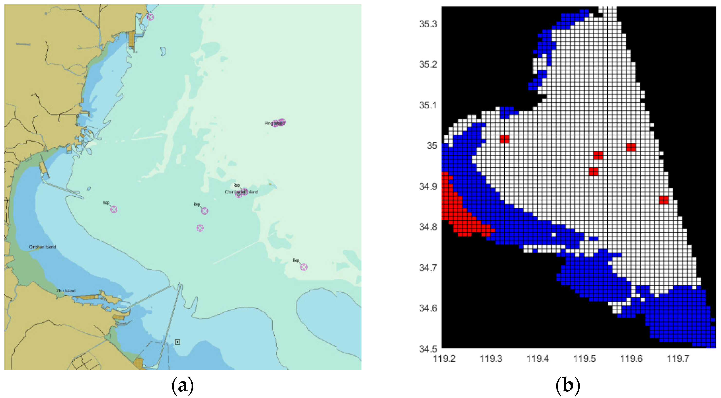
The research area of this paper is Lianyungang and its adjacent waters, which are bounded by Huangdao and Yancheng. Taking it as the original chart data file as shown in Figure 4a, we consider the seaweed farming area in this sea area [29] as an obstacle and rasterize the chart of the sea area. The blue area is the shallow point in the experiment, and the red area is the obstacle, as shown in Figure 4b.
The established dynamic ocean current model of Lianyungang has a north–south span of 172 km and an east–west span of 90 km. In simulation test for ships, the marine vehicle used is a bulk carrier, whose length, breadth, and draft are 185.0 m, 32.26 m, and 12.0 m, respectively.
4.1. Example 1
To verify the effectiveness of the improved ant colony algorithm and compare the difference of the energy consumption of ocean currents between the improved algorithm as well as the traditional one, we chose the current model of Lianyungang with its adjacent sea areas as the test environment and ensured that the ship had the same starting and ending position as well as departure time. The initial speed of the ship was set as 18 km/h, which is the speed of the ship over the ground, and the draft of ship was 12 m. We set [119.28, 35.06] as the starting point (the yellow grid in Figure 5), and [119.67, 34.92] as the end point (the purple grid in Figure 5). To ensure that the improved algorithm and the traditional algorithm were tested under the same conditions, relevant parameters were set to the same initial value, as shown in Table 1.
After the simulation test, the path planning results of the two algorithms were manifested, as shown in Figure 5. Three indicators, which are the ship’s sailing time, path planning distance, and current energy consumption, were applied as evaluation criteria to compare the performance of the two algorithms. According to the path planning results in Figure 5, three performance indicators of the two algorithms are obtained, as demonstrated in Table 2.
The post-smoothing process of the path consists of two parts. Firstly, through applying the improved ant colony algorithm and the improved Bresenham algorithm, the initial path is shortened and the number of vertices and polylines in the path is reduced. Then, the remaining vertices of the first smoothing are eliminated by implementing the principle of cubic B-spline curve.
Different optimization results were obtained by changing the number of turns (number of vertices) of the improved ant colony algorithm, and the specific results are shown in Figure 5. From the simulation results in Figure 5a, it can be seen that the initial path searched out by the improved ant colony algorithm has a large number of broken points and broken lines. After the second-level smoothing of the cubic B-spline curve, the broken lines and broken points were eliminated. This is beneficial for realizing the continuity of speed as well as acceleration during the navigation of the ship and could also avoid the energy consumption when ship turns the rudder, so this design strategy matches our expectation.
Both path planning methods chose the same start and end point during the simulation. The energy consumption of the traditional ant colony algorithm and the optimized one were obtained on the basis of the above environment as well as the speed of the ship. Using the cubic B-spline curve method, the above-mentioned path points were subjected to secondary smoothing, and we calculated the energy saving rate of the optimized ant colony algorithm compared to the traditional one. The formula of calculating the energy-saving rate is as follows.
where EACO is the ocean current energy consumption of the improved algorithm. ACO is the ocean current energy consumption of the traditional algorithm. rate is the energy saving rate.
The traditional ant colony algorithm is oriented by the path length, while the optimized ant colony algorithm considering the influence of the ocean current is oriented by the energy consumption cost. A path with low current energy consumption does not necessarily indicate a short path length, and, likewise, short path lengths do not imply low energy consumption. As shown in Figure 5, the traditional ant colony algorithm considers the influence of the ocean current and is oriented by the optimal path length, and it selects the area with large current resistance relative to the sailing direction. On the basis of continuous experiments on the optimized ant colony algorithm, the path with less energy consumption is selected. The reason why the energy consumption becomes lower while the path length increases is that the energy consumption of bypassing sea areas with high current resistance is far less than the sum of the additional energy consumption resulted by passing through the sea area with large current resistance plus the normal energy consumption. Meanwhile, the longer sailing time is due to the longer path length. In conclusion, experiments proved that the optimized ant colony algorithm has a longer navigation time and an energy saving rate at about 3.326%.
4.2. Example 2
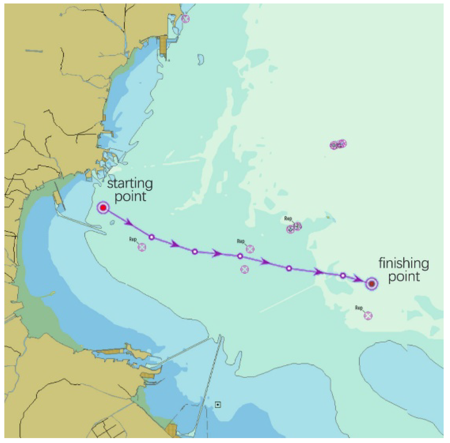
The above experiment is to compare the optimized ant colony algorithm with the traditional ant colony algorithm to verify the practical significance of the energy-saving route. In experiment 2, we choose to calculate the energy consumption of the ship master’s customary route at the same starting and ending position, departure time, and the same departure speed. As shown in Figure 6, it is compared with the energy consumption of the optimized ant colony algorithm.
After the algorithm simulation test, the path planning results of the two algorithms are shown in Figure 6 and Figure 5a. We used the energy consumption of ocean currents to compare the difference between the two, and the results are shown in Table 3.
The same start and end points were selected during the simulation for both routes. Based on the above environment and the speed of the ship, the ship master’s customary route and the energy consumption of the optimized ant colony algorithm were obtained. Using the cubic B-spline curve method, the path points of the optimized ant colony algorithm were subjected to quadratic smoothing. We calculated the energy saving rate of the optimized ant colony algorithm relative to the master’s customary route.
As shown in Figure 5a, the optimized ant colony algorithm considers the influence of the ocean current and selects the area with low resistance to the ocean current relative to the sailing direction. Compared with the ship master’s customary routes, this route has a “detour” phenomenon, but the ant colony algorithm is optimized to find a path with less energy consumption. Experiments show that the optimized ant colony algorithm’s route has an energy saving rate of about 2.709% compared to the customary route.
It can be seen that the planned path with the low energy consumption has distinct practical significance. Similarly, compared with the ship master’s customary paths, the optimal path for the corresponding energy consumption planned by the optimized ant colony algorithm achieved satisfactory results.
5. Conclusions
An improved ant colony algorithm that can calculate the optimal path in real time according to the ocean current environment is proposed for energy saving in this paper. Through the simulation test of the current model of the dynamic change process of the ocean current in the sea area of Lianyungang, it is shown that the improved ant colony algorithm inferred that the current environment can well adapt to the complex and changeable marine environment. Based on this path planning method, the ship can adjust the course according to the calculation results of the model at the time of departure to meet the requirement of saving energy during sailing at sea. The path adjustment algorithm has achieved an energy-saving rate of 3.326% in the simulation test in Lianyungang. In experiment 2, we compared the energy consumption of the master’s customary route with the energy consumption optimized by the ant colony algorithm to verify the practical significance of the energy-saving route. The energy-saving rate of ocean current energy consumption reached 2.709%, which has certain practical significance. In the future, the optimized ant colony algorithm can be further combined with dynamic obstacle avoidance, which has a wide range of application values. Afterwards, more environmental factors would be taken account in this study to stimulate a more realistic application in the navigation field.
Author Contributions
Conceptualization, Y.D. and R.L.; methodology, R.L.; chart data extraction, H.S.; validation, L.C.; customary route plan design, H.S.; algorithm programming, H.S.; data curation, Y.D.; writing—original draft preparation, Y.D.; writing—review and editing, R.L. and J.L.; supervision, R.L.; funding acquisition, R.L. All authors have read and agreed to the published version of the manuscript.
Funding
This research was funded by the National Natural Science Foundation of China (52171346), the Natural Science Foundation of Guangdong Province (2021A1515012618), the special projects of key fields (Artificial Intelligence) of Universities in Guangdong Province (2019KZDZX1035), the scientific research program for university of Guangzhou Education Bureau (202032779), and program for scientific research start-up funds of Guangdong Ocean University (R19055).
Institutional Review Board Statement
Not applicable.
Informed Consent Statement
Not applicable.
Data Availability Statement
Not applicable.
Conflicts of Interest
The authors declare no conflict of interest.
References
- Jia, Q.; Liao, Y.; Xu, P.; Wang, Z.; Pang, S.; Li, X. Long-Endurance Dynamic Path Planning Method of NSV Considering Wind Energy Capture. J. Mar. Sci. Eng. 2021, 9, 878. [Google Scholar] [CrossRef]
- Peng, Z.; Wang, J.; Wang, D.; Han, Q.-L. An Overview of Recent Advances in Coordinated Control of Multiple Autonomous Surface Vehicles. IEEE Trans. Ind. Inform. 2021, 17, 732–745. [Google Scholar] [CrossRef]
- Ma, Y.; Hu, M.; Yan, X. Multi-objective path planning for unmanned surface vehicle with currents effects. ISA Trans. 2018, 75, 137–156. [Google Scholar] [CrossRef]
- Zhao, Y.; Li, W.; Shi, P. A real-time collision avoidance learning system for Unmanned Surface Vessels. Neurocomputing 2016, 182, 255–266. [Google Scholar] [CrossRef]
- Lee, H.-J.; Rhee, K.P. Development of Collision Avoidance System by Using Expert System and Search Algorithm. Int. Shipbuild. Prog. 2001, 48, 197–212. [Google Scholar]
- Namgung, H. Local Route Planning for Collision Avoidance of Maritime Autonomous Surface Ships in Compliance with COLREGs Rules. Sustainability 2022, 14, 198. [Google Scholar] [CrossRef]
- Tanakitkorn, K.; Wilson, P.A.; Turnock, S.R.; Phillips, A.B. Grid-based GA path planning with improved cost function for an over-actuated hover-capable AUV. In Proceedings of the 2014 IEEE/OES Autonomous Underwater Vehicles (AUV), Oxford, MS, USA, 6–9 October 2014; IEEE: Piscataway, NJ, USA, 2014; pp. 1–8. [Google Scholar]
- Zhang, Q. A Hierarchical Global Path Planning Approach for AUV Based on Genetic Algorithm. In Proceedings of the 2006 International Conference on Mechatronics and Automation, Luoyang, China, 25–28 June 2006. [Google Scholar]
- Chang, Z.-H.; Tang, Z.-D.; Cai, H.-G.; Shi, X.-C.; Bian, X.-Q. GA path planning for AUV to avoid moving obstacles based on forward looking sonar. In Proceedings of the 2005 International Conference on Machine Learning and Cybernetics, Guangzhou, China, 18–21 August 2005. [Google Scholar]
- Zeng, Z.; Lammas, A.; Sammut, K.; He, F. Optimal path planning based on annular space decomposition for AUVs operating in a variable environment. In Proceedings of the 2012 IEEE/OES Autonomous Underwater Vehicles (AUV), Southampton, UK, 24–27 September 2012. [Google Scholar]
- Khan, F.A.; Turgut, D.; Boloni, L. Optimizing Resurfacing Schedules to Maximize Value of Information in UWSNs. In Proceedings of the 2016 IEEE Global Communications Conference (GLOBECOM), Washington, DC, USA, 4–8 December 2016. [Google Scholar]
- Sun, J.; Liu, X. Path Plan of Unmanned Underwater Vehicle Using Particle Swarm Optimization; Atlantis Press: Amsterdam, The Netherlands, 2015. [Google Scholar]
- Ma, Y.; Zamirian, M.; Yang, Y.; Xu, Y.; Zhang, J. Path Planning for Mobile Objects in Four-Dimension Based on Particle Swarm Optimization Method with Penalty Function. Math. Probl. Eng. 2013, 2013, 1–9. [Google Scholar] [CrossRef] [Green Version]
- Cao, X.; Zhu, D.; Yang, S.X. Multi-AUV Target Search Based on Bioinspired Neuro dynamics Model in 3-D Underwater Environments. IEEE Trans. Neural Netw. Learn. Syst. 2016, 27, 2364–2374. [Google Scholar] [CrossRef] [PubMed]
- Shen, J.; Shi, J.; Xiong, L. A Route Planning Method for Underwater Terrain Aided Positioning Based on Gray Wolf Optimization Algorithm; Springer International Publishing: Cham, Switzerland, 2016. [Google Scholar]
- Qu, N.; Chen, G.; Shen, Y. A Three-Dimensional Path Planning System for AUV Diving Process Considering Ocean Current and Energy Consumption. In Proceedings of the OCEANS 2021, San Diego, CA, USA, 20–23 September 2021. [Google Scholar]
- Dong, L.; Li, J.; Xia, W.; Yuan, Q. Double ant colony algorithm based on dynamic feedback for energy-saving route planning for ships. Soft Comput. 2021, 25, 5021–5035. [Google Scholar] [CrossRef]
- Pan, X.; Wu, X.; Hou, X. Research on Global Path Planning for Autonomous Underwater Vehicle Considering Ocean Current. In Proceedings of the 2018 2nd IEEE Advanced Information Management, Communicates, Electronic and Automation Control Conference (IMCEC), Xi’an, China, 25–27 May 2018. [Google Scholar]
- Perez-Carabaza, S.; Portas, E.B.; Lopez-Orozco, J.A.; de la Cruz, J.M. Ant colony optimization for multi-UAV minimum time search in uncertain domains. Appl. Soft Comput. 2018, 62, 789–806. [Google Scholar] [CrossRef]
- Zadeh, S.M.; Powers, D.M.; Sammut, K. An autonomous reactive architecture for efficient AUV mission time management in realistic dynamic ocean environment. Robot. Auton. Syst. 2017, 87, 81–103. [Google Scholar] [CrossRef]
- Lim, K.K.; Ong, Y.-S.; Lim, M.H.; Chen, X.; Agarwal, A. Hybrid ant colony algorithms for path planning in sparse graphs. Soft Comput. 2008, 12, 981–994. [Google Scholar] [CrossRef]
- Cai, W.; Zhang, M.; Zheng, Y.R. Task Assignment and Path Planning for Multiple Autonomous Underwater Vehicles Using 3D Dubins Curves. Sensors 2017, 17, 1607. [Google Scholar] [CrossRef] [PubMed] [Green Version]
- Stützle, T.; Dorigo, M. A short convergence proof for a class of ant colony optimization algorithms. IEEE Trans. Evol. Comput. 2002, 6, 358–365. [Google Scholar] [CrossRef]
- Jing, C. Research on AUV Path Planning Method in Complex Environment; Ocean University of China: Qingdao, China, 2011. [Google Scholar]
- Jianhua, D. Research on Optimization Algorithm for Path Planning of Underwater Robots; Harbin Engineering University: Harbin, China, 2009. [Google Scholar]
- Hu, D.; Wang, M.; Yao, S.; Jin, Z. Study on the Spillover of Sediment during Typical Tidal Processes in the Yangtze Estuary Using a High-Resolution Numerical Model. J. Mar. Sci. Eng. 2019, 7, 390. [Google Scholar] [CrossRef] [Green Version]
- Dorigo, M.; Maniezzo, V.; Colorni, A. Ant system: Optimization by a colony of cooperating agents. IEEE Trans. Syst. Man Cybern. Part B 1996, 26, 29–41. [Google Scholar] [CrossRef] [PubMed] [Green Version]
- Willmott, C.J. On the Validation of Models. Phys. Geogr. 1981, 2, 184–194. [Google Scholar] [CrossRef]
- Xu, H.; Zhang, Y.; Chen, Z.; Chu, J. Remote sensing monitoring and analysis of seaweed cultivation area in Lianyungang sea area in recent 10 years. Mod. Surv. Mapp. 2019, 42, 10–14. [Google Scholar]
Figure 1.
Schematic diagram of the motion of grids with currents.
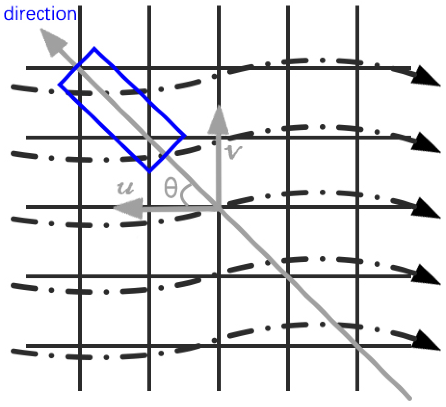
Figure 2.
Study area and mesh.

Figure 3.
Validation of water level.
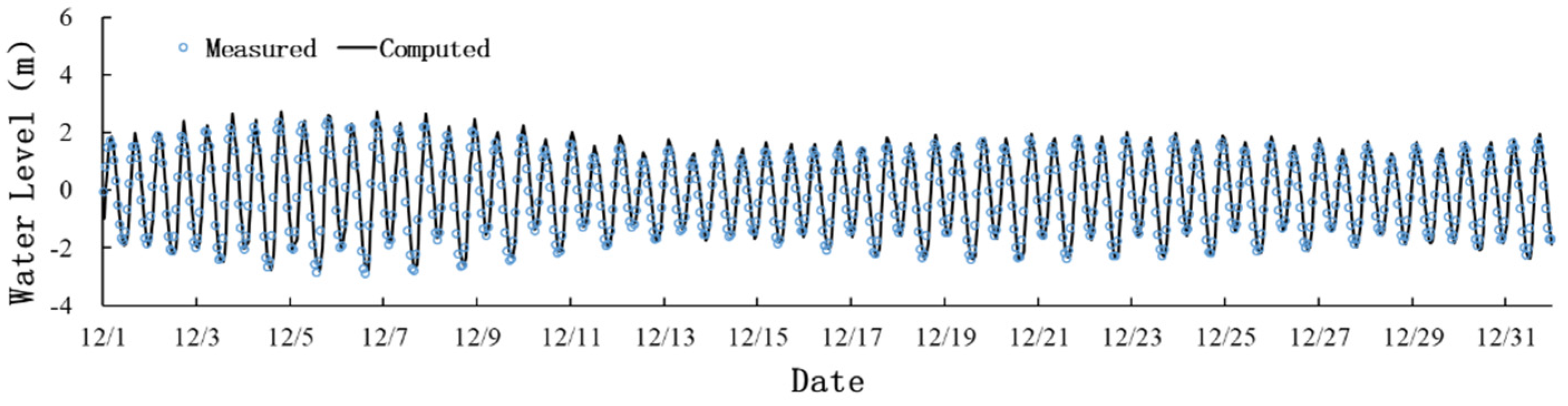
Figure 4.
(a) A sea area in EC, and (b) grid map of the sea area.

Figure 5.
(a) Energy consumption of improved ant colony algorithm, and (b) energy consumption of traditional ant colony algorithm.
Figure 5.
(a) Energy consumption of improved ant colony algorithm, and (b) energy consumption of traditional ant colony algorithm.
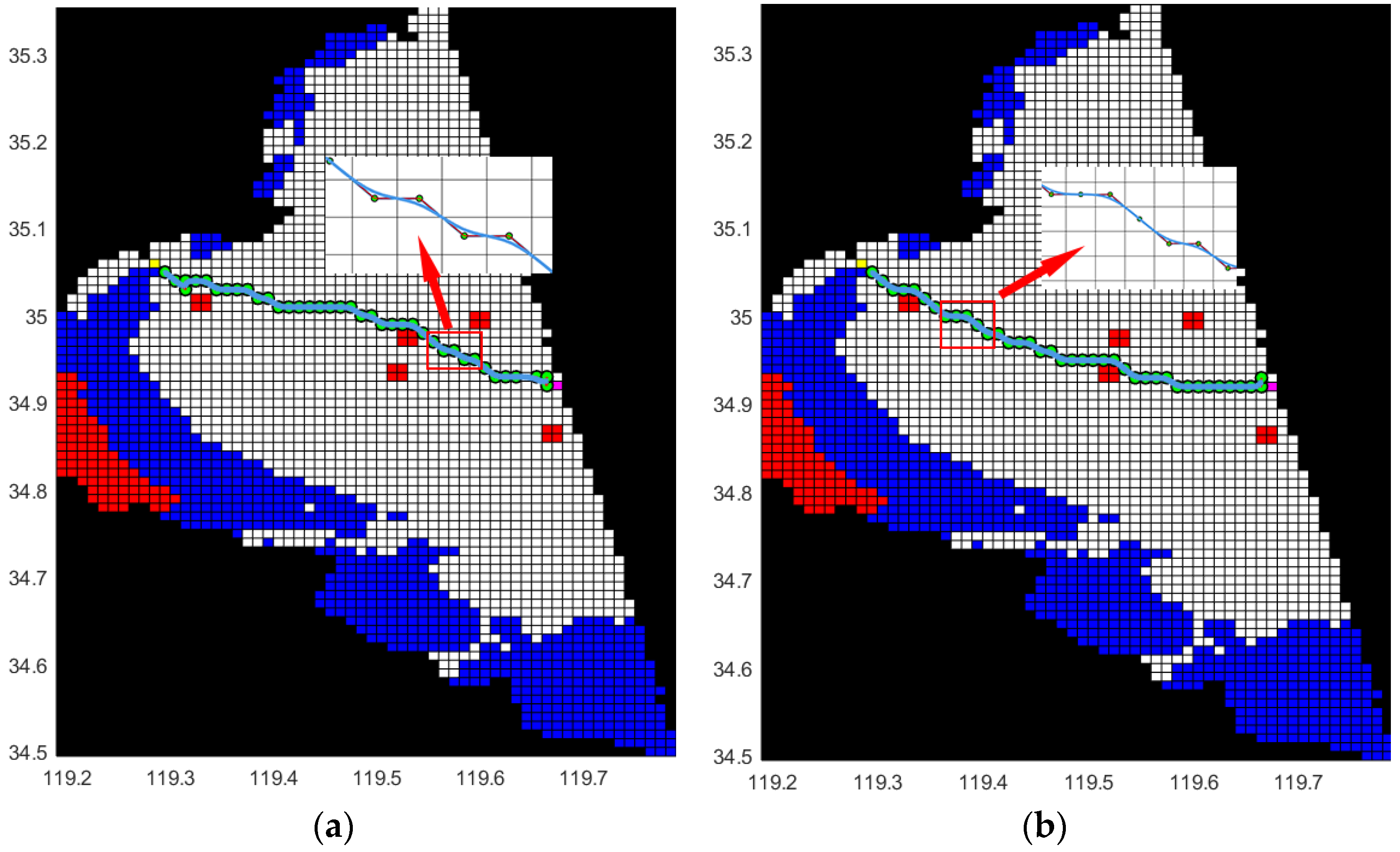
Figure 6.
The customary route by ship master.

Table 1.
Related parameter settings.
| Parameters | Number |
|---|---|
| 0.4 | |
| 5 | |
| 0.1 | |
| 1.02 × 10³ | |
| 15.72 |
Table 2.
Index comparison between improved and traditional ant colony algorithm.
| Indicator | Sailing Time | Path Planning Distance | Energy Consumption |
|---|---|---|---|
| Improved | 9171.0 s | 46,491.7 m | 102,931,597,865.8 J |
| Traditional | 9037.2 s | 45,813.4 m | 106,472,685,239.8 J |
Table 3.
Index comparison between improved ant colony algorithm and ship master’s customary route.
| Indicator | Sailing Time | Path Planning Distance | Energy Consumption |
|---|---|---|---|
| Improved | 9171.0 s | 46,491.7 m | 102,931,597,865.8 J |
| Customary route | 9103.8 s | 46,013.4 m | 105,797,842,971.5 J |
Publisher’s Note: MDPI stays neutral with regard to jurisdictional claims in published maps and institutional affiliations. |
© 2022 by the authors. Licensee MDPI, Basel, Switzerland. This article is an open access article distributed under the terms and conditions of the Creative Commons Attribution (CC BY) license (https://creativecommons.org/licenses/by/4.0/).
Share and Cite
MDPI and ACS Style
Ding, Y.; Li, R.; Shen, H.; Li, J.; Cao, L. A Novel Energy-Saving Route Planning Algorithm for Marine Vehicles. Appl. Sci. 2022, 12, 5971. https://doi.org/10.3390/app12125971
AMA Style
Ding Y, Li R, Shen H, Li J, Cao L. A Novel Energy-Saving Route Planning Algorithm for Marine Vehicles. Applied Sciences. 2022; 12(12):5971. https://doi.org/10.3390/app12125971
Chicago/Turabian StyleDing, Ying, Ronghui Li, Haiqing Shen, Jiawen Li, and Liang Cao. 2022. "A Novel Energy-Saving Route Planning Algorithm for Marine Vehicles" Applied Sciences 12, no. 12: 5971. https://doi.org/10.3390/app12125971
Note that from the first issue of 2016, this journal uses article numbers instead of page numbers. See further details here.