Article

Feature Selection to Predict LED Light Energy Consumption with Specific Light Recipes in Closed Plant Production Systems

by
Martín Montes Rivera
1,*,
Nivia Escalante-Garcia
2,*,
José Alonso Dena-Aguilar
3,
Ernesto Olvera-Gonzalez
2 and
Paulino Vacas-Jacques
3
1
Dirección de Posgrados e Investigación, Universidad Politécnica de Aguascalientes, Calle Paseo San Gerardo #201, Fracc. San Gerardo, Aguascalientes 20342, Mexico
2
Laboratorio de Iluminación Artificial, Tecnológico Nacional de México/IT de Pabellón de Arteaga, Carretera a la Estación de Rincón Km. 1, Aguascalientes 20670, Mexico
3
Departamento de Ingenierías, Tecnológico Nacional de México/IT de Pabellón de Arteaga, Carretera a la Estación de Rincón Km. 1, Aguascalientes 20670, Mexico
*
Authors to whom correspondence should be addressed.
Appl. Sci. 2022, 12(12), 5901; https://doi.org/10.3390/app12125901
Submission received: 3 May 2022 / Revised: 19 May 2022 / Accepted: 26 May 2022 / Published: 9 June 2022
(This article belongs to the Topic Artificial Intelligence and Sustainable Energy Systems)

Abstract

:
The use of closed growth environments, such as greenhouses, plant factories, and vertical farms, represents a sustainable alternative for fresh food production. Closed plant production systems (CPPSs) allow growing of any plant variety, no matter the year’s season. Artificial lighting plays an essential role in CPPSs as it promotes growth by providing optimal conditions for plant development. Nevertheless, it is a model with a high demand for electricity, which is required for artificial radiation systems to enhance the developing plants. A high percentage (40% to 50%) of the costs in CPPSs point to artificial lighting systems. Due to this, lighting strategies are essential to improve sustainability and profitability in closed plant production systems. However, no tools have been applied in the literature to contribute to energy savings in LED-type artificial radiation systems through the configuration of light recipes (wavelengths combination. For CPPS to be cost-effective and sustainable, a pre-evaluation of energy consumption for plant cultivation must consider. Artificial intelligence (AI) methods integrated into the prediction crucial variables such as each input-variable light color or specific wavelengths like red, green, blue, and white along with light intensity (quantity), frequency (pulsed light), and duty cycle. This paper focuses on the feature-selection stage, in which a regression model is trained to predict energy consumption in LED lights with specific light recipes in CPPSs. This stage is critical because it identifies the most representative features for training the model, and the other stages depend on it. These tools can enable further in-depth analysis of the energy savings that can be obtained with light recipes and pulsed and continuous operation light modes in artificial LED lighting systems.

1. Introduction

1.1. LED Lights in Closed Plant Production Systems

Agriculture in 2050 will have to produce almost 50% more output to meet the demand for food supplies, presenting it with a crucial challenge in meeting the increase in demand [1]. Technological development and innovation can offer alternatives to ensure food security sustainably. The use of closed growth environments, such as greenhouses, plant factories, and vertical farms [2,3,4,5,6], represents a sustainable alternative for fresh food production. In closed plant production systems (CPPSs), several variables can be controlled and optimized, such as water, fertilizers, CO2 injection, and temperature, as well as the quantity and quality of light thus ensuring minimum greenhouse gas emissions [3]. CPPSs allow growing of any plant variety, no matter the season of the year. Artificial lighting plays an essential role in CPPSs, as it promotes growth by providing optimal conditions for plant development. LEDs are energy-efficient replacements that contribute to plant growth in agriculture. An outstanding advantage of LED lamps is their ability to operate with specific wavelengths (λ) that considerably reduce energy consumption. LEDs regularly generate continuous light. Likewise, they can radiate pulsed light (on/off in microseconds (µs)) with high power and low energy consumption at a specific frequency and duty cycle without upsetting the vegetative development of plants [4,7,8]. LED technology can produce different colors of light—that is, different qualities—called light recipes (different wavelength combinations). The wavelength combinations (red, blue, green, ultraviolet, and infrared) and the photosynthetic photon flux density (PPFD, given in µmol m−2 s−1) are the components that constitute the light recipes. Light recipes impact crop growth from branching to flowering; optimize the biomass; and increase the antioxidant capacity levels of calcium, potassium, magnesium, chlorophyll, iron, vitamins A, B, and E, and other substances [7,8,9]. Crop quality and productivity rely upon the time and the light quantity supplied to the plants.
CPPSs can offer several advantages (improved management control of all variables involved—temperature, CO2, radiation—and increased productivity, growth, and yield) and generate an impact on humanity. Nevertheless, it is a model with a high demand for electricity for the artificial radiation systems needed to enhance the developing plants. Environmental control (refrigeration), the air required to remove the heat produced, and artificial lighting account for approximately 32%, 11%, and 57% of the total energy demand, respectively [10]. Furthermore, according to Avgoustaki and Xydis [11], the artificial lighting system accounts for 80% of the electrical demand, since the overall operability of the CPPS accounts for 40% of the total energy consumption.
Innovative approaches, such as fluid dynamics, evolutionary algorithms [12,13], the derivative integral model, and derivative model [14,15,16], control the resources in CPPSs. Artificial neural networks predict weather conditions and energy consumption [13,14,15,17]. Other techniques predict energy consumption performance for plant production [18,19]. Finally, other techniques focus on in the optimization of resources and reducing energy demand in CPPSs [20,21].

1.2. Machine-Learning Modeling

Physical modeling approaches are the most common approaches for predicting system behaviors, but they rely on descriptions of physics concepts. Thus, they tend to be complex, as the detail of the model increased. Therefore, as the principle of Occam’s razor states, physical modeling must balance complexity with assumptions in order to produce simplified and representative models [22,23].
On the other hand, artificial intelligence (AI) researchers have proposed several techniques that allow automatic generation of the models and equations based on measurements arranged in datasets. Furthermore, machine learning (ML), a field of AI, applies deterministic and heuristic methods to produce models with less complexity established in the raw measurements [22].
During the last two decades, ML models have exhibited high effectivity, accuracy, and performance in several fields, including energy applications. Furthermore, ML results for modeling have motivated researchers to apply its models to accurately predict the behavior of physical phenomena [22,23,24,25,26,27,28,29,30].
The ML modeling process can involve several stages, depending on its application, but a general description would include collecting data, preprocessing data, building a model, training, and testing. Furthermore, all the stages must be continually tuned to improve the results; i.e., the stages can repeatedly change across the entire process if the model requires efficiency improvements, as represented in Figure 1 [22].

1.2.1. Collecting Data

ML modeling uses algorithms, statistics, and measurements structured in a dataset to identify the process behaviors and mimic them in a model [31]. The data generation stage depends on the processes contained in the chosen model. They may include electrical, mechanical, optical, thermal, psychic, or chemical variables [22,24,25,32,33]; derive from statistical analysis [26,27]; or be constructed with text, multimedia, or even real-time reports [32,33,34,35]. Nevertheless, the datasets can be associated with a specific time and/or frequency domain [36,37].

1.2.2. Preprocessing Data

After collecting and structuring the dataset, its variables need to be cleaned, processed, and filtered for the ML model. The processing stage includes several techniques, which can be human- or AI-designed, and they depend on the nature of the training data. For example, in natural language processing with text, preprocessing removes capitals [38]; in signal processing, wavelet transforms separate signals into their main components [39]; in image processing, convolution with the image filters extracts features [40]; in big data and data mining, dimensionality reduction is achieved [41].
The preprocessing data stages include normalization based on algorithms, such as MIN-MAX normalization, decimal scaling, and Z-scores; filtering redundant and inconsistent data; transformations such as linear, quadratic, polynomial, and histogram transformations; removing noisy data with techniques such as ensemble filtering, cross-validated filtering, and interactive partitioning; feature selection with exhaustive, heuristic, filter, and wrapper methods; and discretization to change from analog systems to digital ones [42].
Input features in ML modeling are representative when their information affects the output of the modeled system. Additionally, removing characteristics that are irrelevant or have low correlations from the results produces search spaces with lower complexity, boosting the capabilities of the training algorithm and improving the final model’s efficiency [43,44].
One of the most used commonly techniques for removing redundant and inconsistent data in the second stage is feature Selection (FS). FS also makes it possible to reduce size, increase the efficiency and accuracy of predictive learning, and reduce the complexity of the final model [42]. The different FS approaches reported in the literature are constituted theoretically and apply methods such as filtering, wrapping, and embedding through techniques involving search algorithms, statistical criteria, and information, distance, dependency, and consistency measures [42].

1.2.3. Building Model

ML includes several models for predicting behavior that are supported by statistics and artificial intelligence. Different proposals have obtained different results depending on the ML model’s application. The most common models are artificial neural networks, evolutionary algorithms, swarm intelligence algorithms, decision trees, naive Bayesian algorithms, logistic regression, fuzzy systems, gradient boosting machines, support vector machines, support vector regression, random forest algorithms, AdaBoost, simulated annealing, and hybrids of these models [22,24,26,27,28,31,34,44].

1.2.4. Training Model

Each ML model tunes its internal parameters with a training algorithm designed for the learning type. The most common learning types are supervised, unsupervised, reinforced, semi-supervised, transductive, self-trained, ensemble learning, boosting, and generative [31].

1.2.5. Testing Model

The metrics used to evaluate quality in the process of ML modeling depend on the nature of the model, which may be for classification or regression. In regression models, the metrics quantify the reliability of the model and the error between the model output and the real-world system. The most common regression metrics are the root mean square error (RMSE), mean error (ME), mean absolute error (MAE), mean average percentage error (MAPE), and the Nash coefficients E and R 2 [22,44].

1.3. Feature Selection

As mentioned in Section 1.2.2, feature selection is one of the most critical stages of ML modeling since it makes it possible to identify the best relation to the required complexity of the model and its quality at the preprocessing stage. In addition, feature selection makes it possible to find the more representative inputs in the real-world system and to eliminate no representative inputs or those that are redundant. ML models and training algorithms that consider only representative features improve their efficiency and reduce the time required for training [26,27,38,45]. A feature is an observable property in a system. Feature selection aims to select a specific subset of features that maximize the performance of the ML model.
The feature selection (FS) used here applied one of the most common techniques for removing irrelevant data, reducing dimensionality, increasing predictive accuracy and learning efficiency, and reducing the complexity of the final model [42]. Although there are different approaches for FS, all have theoretical support in their use of different methods, such as filtering, wrapping, and embedding, and involve techniques that use search algorithms, statistical criteria, and information, distance, dependence, and consistency measures [42]. The aim was to use linear and nonlinear methods to implement FS with a dataset acquired from an illumination radiation system.
This paper focuses on the feature selection stage in order to train a regression model to predict energy consumption in LED lights with specific light recipes in CPPSs. This stage is critical because it identifies the most representative features for training the model, and the other stages depend on it. These tools can enable further in-depth analysis of the energy savings that can be obtained with light recipes and pulsed and continuous light operation modes in artificial LED lighting systems.

2. Materials and Methods

2.1. Lighting System Features

The Artificial Lighting Laboratory (LIA) at Instituto Tecnológico de Pabellón de Arteaga in Aguascalientes, Mexico, developed the lighting system. An array of eight lamps formed the artificial lighting system. The wattage of each lamp was 25 watts. The ultra-bright LEDs emitted continuous and pulsed irradiation with different qualities (red, blue, green, and white). A programmed controller (a field-programmable gate array (FPGA)) allowed us to configure functions such as pulse frequency, duty cycle, intensity, wavelength, and on–off time.

2.2. Construction of Experiment

This study evaluated 10 light recipes from the literature, as can be seen in Figure 2. After that, the LED artificial radiation system was configured for continuous and pulsed emission to generate the first dataset (see table at the top of figure) to be analyzed. The intensities parameters were 50, 65, 80, 95, 110, 125, 140, 155, 170, and 185 µmol m−2 s−1, as determined by a quantum sensor, and the frequency was set to 100, 500, and 1000 Hz with 40%, 50%, 60%, 70%, 80%, and 90% duty cycles for different treatments.
In the generation of the second dataset, four different light recipes were set at intensities of 60, 70, 85, 90, 90, 100, 120, 130, 150, 160, and 180 µmol m−2 s−1, the frequency was set at 100, 500, and 1000 Hz, and duty cycles were randomly selected at 60%, 70%, and 80%, depending on the treatment (see table at the bottom of Figure 2).
The artificial illumination system included 14 light recipes (see tables in Figure 2) with all combinations of parameters. After 60 min of radiation, we registered the measurements for the energy demand with a hook-on AC ammeter (Peak Teach, Salerno, Italy) in watts × hours (Wh). Then, the artificial radiation system was turned off for 15 min to cool down.

2.3. Min-Max Normalization

Normalization linearly transforms variables within specific ranges based on the minimum and maximum median absolute deviations of the variable values, avoiding changes to priorities in the variables because of the scale. Equation (1) represents the standard deviation required in the transformation as X s t d , and Equation (2) indicates the variable scaling [46,47].
X s t d = x X m i n X m a x X m i n
X s c a l e d = X s t d × ( X m a x X m i n ) + X m i n
where X s c a l e d is the new value transformed from the original value x X and X m a x and X m i n are the maximum and minimum values, respectively.

2.4. Pearson Correlation

This association method’s primary goal is to identify two or more correlated variables [45].
The Pearson correlation coefficient measures the degree of correlation between two variables in a linear approach. Let X and Y be those variables, with measurements given by { x 1 , x 2 , x 3 , ... , x n } and { y 1 , y 2 , y 3 , ... , y n } and means x ¯ and y ¯ . Then, the Pearson coefficient is given by Equation (3) [42].
ρ ( X , Y ) =   i = 1 n ( x i x ¯ ) ( y i y ¯ ) [ i = 1 n ( x i x ¯ ) 2 i = 1 n ( y i y ¯ ) 2 ] 1 2
A Pearson coefficient with the range ρ = [ 1 , 1 ] represents the level of correlation when ρ is positive and correlation is direct, and the negative is the inverse [42].
When two variables are highly correlated, one can be redundant. The Pearson correlation works only for linear relations and results in incorrectly measured correlations for nonlinear systems. When classifying with binary outputs, it is possible to identify using Pearson coefficients how an attribute correlates with the target class [42].
Additionally, one can perform a correlation statistical significance test using the p v a l u e coefficient, such as a test of the probability that the correlation coefficient ρ is a wrong hypothesis; for example, as a convention from the literature, if p v a l u e > 0.05 , it is unreliable. The alternatives for such a determination include statistical tests, such as the t v a l u e , variance analysis (ANOVA), and 1 t a i l e d or 2 t a i l e d tests [48].

2.5. Variance Threshold

This method is used to identify features with variance. The features eliminated based on variance are those with zero value, near to zero value, or below a specific threshold [49,50,51].
The variability in a group given with { x 1 , x 2 , x 3 , ... , x n } is the standard error; in other words, it is the difference between the samples and the average value of the group x ¯ , as in Equation (4) [52].
σ 2 = i = 1 n ( x i x ¯ ) 2 n 1

2.6. Mutual Information Gain

Feature selection with mutual information gain enables the discrimination of features based on their interaction measurement, both for linear and nonlinear models [53]. Mutual information measures the uncertainty based on the entropy H of one variable while observing the other one. Let X be a random variable with values { x 1 , x 2 , x 3 , ... , x n } ; its entropy is given by Equation (5) [54].
H ( X ) = i = 1 n P ( x i ) l o g 2 [ P ( x i ) ]
Let Y be an output variable with values { y 1 , y 2 , y 3 , ... , y n } and let X be a features array with values { x 1 , x 2 , x 3 , ... , x n } ; H ( X | Y ) is then given by Equation (6) [54].
H ( X Y ) = j = 1 n [ P ( x i ) ] i = 1 n P ( x i y j ) log 2 [ P ( x i y j ) ]
The mutual information in Equation (7) measures the reduction in the uncertainty of X given Y [54,55].
M I ( X | Y ) = H ( X ) H ( X | Y )

2.7. Univariate Linear F-Regression Selection

This method uses a linear model to measure the degree of linear dependence between two random variables; in other words, it measures the significance of a feature in a linear model [56].
The F-regression equations use the null hypothesis H 0 , indicating that the data only intercept the model, and the alternative hypothesis H 1 , indicating the compatibility of the data with the model. The selection of the true hypothesis relies on the F s c o r e given in Equation (8), the explained variance from Equation (9), and the unexplained variance from Equation (10) [56].
F = explained   variance unexplained   variance
explained   variance = i = 1 K n i ( Y ¯ i Y ¯ ) 2 ( K 1 )
unexplained   variance = i = 1 K j = 1 n i ( Y i j Y ¯ i ) 2 ( N K )
where Y i j is the j th observation in the i out group in K , which is the number of out groups. N is the overall sample size and n i is the number of observations.
Additionally, following Section 2.4, one can determine a p v a l u e for the hypothesis conclusion, and, like with the Pearson correlation, if p v a l u e > 0.05 , the conclusion is unreliable [56].

2.8. Sequential Feature Selection

Sequential feature selection algorithms are a subset of wrapper algorithms that use greedy search algorithms. They evaluate a solution with certain features in a specific model and decide which feature to remove based on its quality. This technique can use a feedforward or backward approach; i.e., adding or removing features in the model. Figure 3 displays the searching schema for feedforward and backward sequential selection with three features [57,58].
For this study, backward sequential feature selection served to remove the worst variables in the energy consumption dataset for the LED lamps of a CPPS.

2.8.1. Linear Regression Model

The linear model structure includes Y   n × 1 , where Y = ( y 1 , y 2 , y 3 , ... , y n ) T is the response variable; X   n × p , where X =   ( x 1 , x 2 , x 3 , ... , x n ) represents the design matrix; and x i = ( x i , 1 , x i , 2 , x i , 3 , ... , x i , p ) and β   p × 1 , where n is the number of observations and p is similar to the number of features. Then, the linear regression model is given by Equation (11) [59].
Y = μ + ϵ
where μ = β × X and ϵ is the regression error.
Then, with a given predictor Y and the design matrix X , Equation (12) solves the β model parameters that reduce ϵ [59].
β = ( X T X ) 1 X T Y

2.8.2. Decision Tree Regression Model

Decision trees are hierarchical structures with nodes representing tests of the data with specific attributes and branches representing the test results. Decision tree models include IDS, C4.5, CART, and regression models. For example, the regression decision trees predict continuous random variables by finding the attributes that reduce the mean square error (MSE), obtained with Equation (13) [60].
M S E = 1 n i = 1 n ( y i y ¯ i ) 2
where Y = ( y 1 , y 2 , y 3 , ... , y n ) is the raw data output variable and Y ¯ = ( y ¯ 1 , y ¯ 2 , y ¯ 3 , ... , y n ) represents the decision tree model output [60].
For this application, the regression variable used a decision tree with the energy consumption and the node attributes as the features for the energy consumption dataset.

3. Results

3.1. Energy Consumption Dataset

We registered the power consumption emitted by the artificial lighting system as a function of the light recipe, including parameters such as intensity; R, G, B, and W quality; frequency; and duty cycle. Table 1 represents the first dataset obtained through the process described in Section 2 (Figure 2). The evaluated energy consumption contained different ranges depending on the directly configured parameters. However, applying specific value ranges to the inputs affects the priority assigned to each one.
Endeavoring not to affect the input priorities, a new scaled dataset with min-max normalization was generated according to the equations defined in Section 2.3. Table 2 shows the data obtained after applying the equations corresponding to each input and output variable. The data represent the ranges from 0 to 1 after normalization. A value of 0 corresponds to the minimum value identified for that variable, while 1 is the maximum.

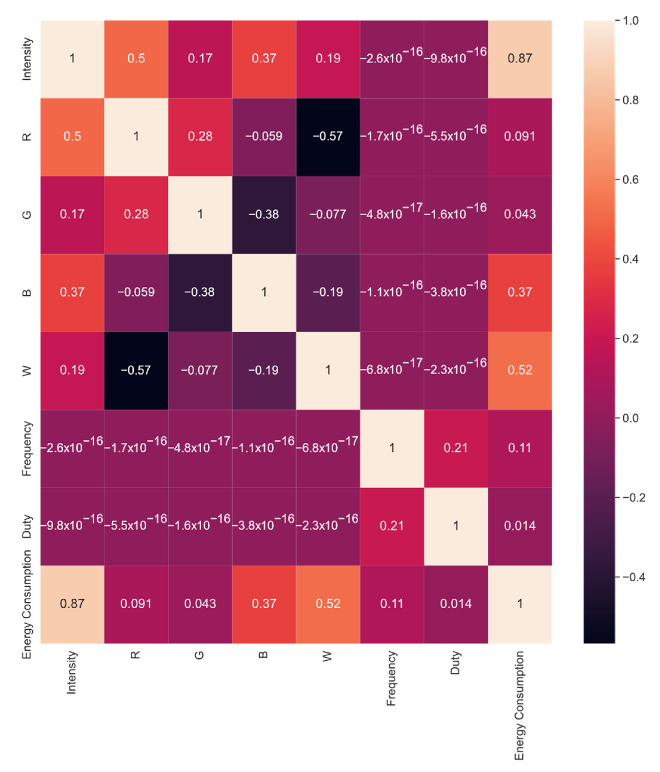
3.2. Person Correlation Results

The next step was determining the Pearson correlation level with the coefficient ρ supported by the statistic test p v a l u e using the equations in Section 2.4. The evidence for Pearson correlation with intensity, R, G, B, W, and frequency was sufficient as p v a l u e 0.05 , but the duty correlation was unreliable because p v a l u e > 0.05 . Thus, duty cycle was the first variable eliminated (Table 3).
Figure 4 shows a correlation heat map of the input variables and the energy consumption output to identify the strongest correlations graphically. There is a lower correlation where the graph color is darker.

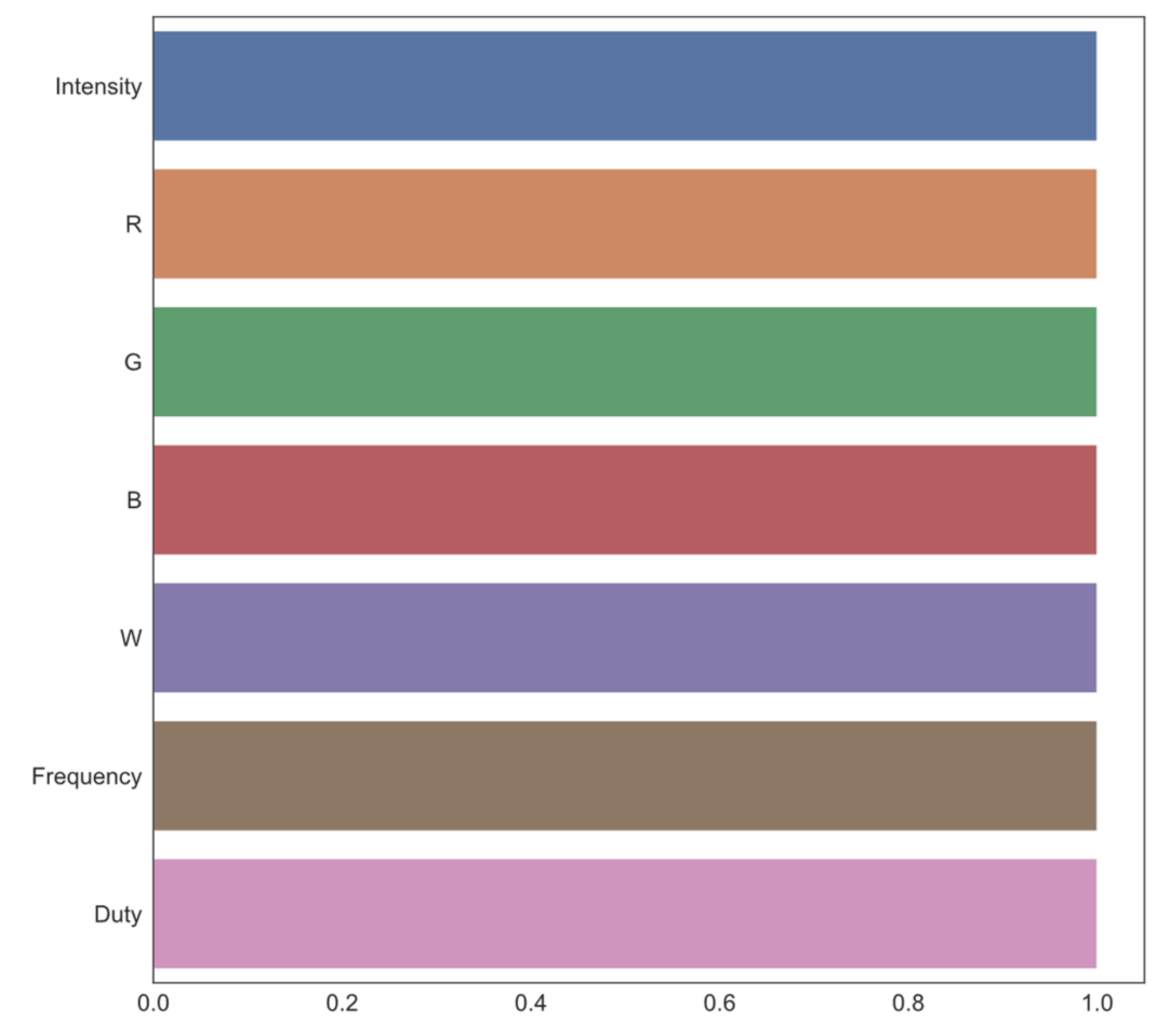
3.3. Variance Threshold Results

The dataset energy consumption variables were dismissed against the variance threshold value as it gradually increased. The method for eliminating the variables with lower variance was described in Section 2.5. Figure 5 indicates the color associated with each variable in the variance threshold selection.
Table 4 displays the feature variance, the threshold value, and a bar plot showing the eliminated variable. Each threshold value was increased by 0.01 steps until a feature was eliminated from the energy consumption dataset.

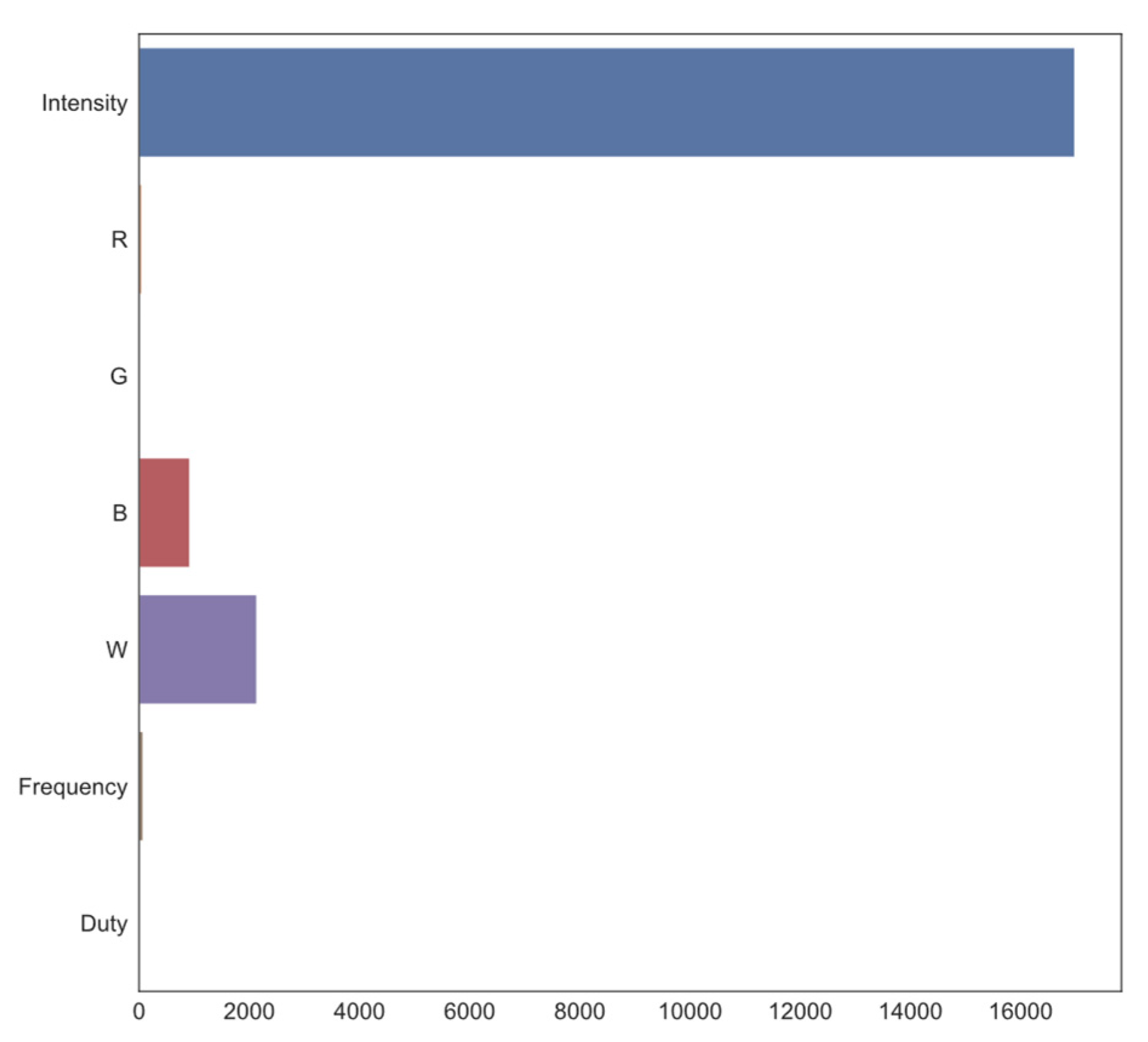
3.4. Mutual Information Gain Results

Mutual information gain feature selection for the energy consumption dataset, set as the output variable, and all the other variables, assigned to the features array, was applied according to the description in Section 2.6. The results of this analysis are represented in Figure 6 and Table 5.

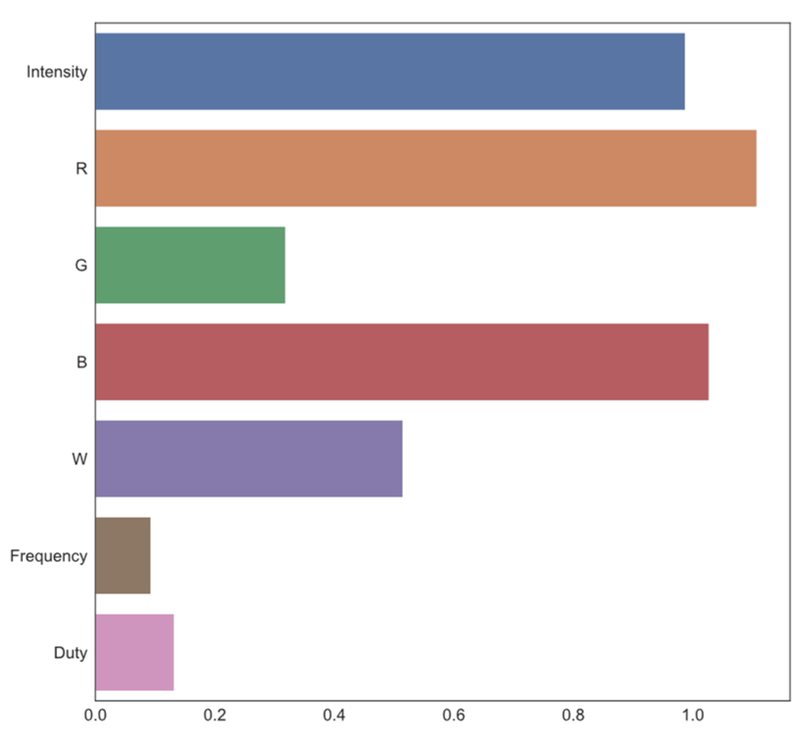
3.5. Univariate Linear F-Regression Results

Once again, feature selection by F-regression in the generated dataset employed the energy consumption, such as the outcome variable in the features array (Section 2.7). Figure 7 displays the F s c o r e value for hypothesis H 0 for each variable in the features array, and Table 6 shows the F s c o r e and p v a l u e calculated by H 0 for all input parameters.
The calculated p v a l u e is indicated in Table 6. The Pearson correlations for intensity, R, G, B, W, and frequency showed reliable results since p v a l u e 0.05 , but the duty cycle correlation was unreliable because p v a l u e > 0.05 ; that is, the duty cycle was the first eliminated.

3.6. Sequential Feature Selection Results

We used backward sequential feature selection under a linear model and a decision tree regression (no linear model). However, implementation of the sequential feature selection through the decision tree may have generated overfitting; thus, a 10-fold cross-validation allowed the recognition of the accepted characteristics by modifying the tree depth from 2 to 5.

3.6.1. Sequential Feature Selection with Linear Regression Model

Table 7 presents the results obtained for the linear regression model (Section 2.8.1) determining the feature elimination sequence, which used as attributes the admitted range from 1 to 6. The table follows the logic of Figure 5, showing each color in the elimination ranking with the variance threshold.

3.6.2. Sequential Feature Selection with Decision Tree Regression Model

The feature recognition through the decision tree regression model used the variance in a specific feature, which ranged from 1 to 6, allowing the elimination order for each input variable (Table 8, Table 9, Table 10 and Table 11) to be obtained from the tree depth configuration. A color image of each feature, following the structure for variance threshold selection, is shown in Figure 5.

4. Discussion

The results obtained require division into linear and nonlinear model selection algorithms. The division generated makes it possible to analyze the results according to the model type and to identify the sequence of each feature. Table 12 and Table 13 show the algorithms by group, the feature selection order, and the mean.
The averages calculated and reported in Table 12 and Table 13 indicate two different behaviors depending on the model performance (linear or nonlinear). Figure 8 shows an alternative way to visualize the performance between linear and nonlinear models.
After dividing the models into linear and nonlinear groups, we validated the ordinal elimination variables on a scale from 1 to 7 and tested the distributions with the Kruskal–Wallis test (Table 14) [61]. The sequence elimination distribution for the proposed models is shown in Figure 9 and Figure 10 (linear and nonlinear models, respectively).
The linear model indicated that the essential characteristic was intensity, while the least significant was the duty cycle (Figure 9 and Table 14). If the appropriate sequence for any variable is required, the mean value can be found in Table 12. This means that the elimination order for the linear models was duty cycle, G, R, W, B, frequency, and intensity.
The nonlinear model found that the most crucial characteristic was intensity, while the least important was W (white color), with sufficient significance p < 0.05 . If the correct sequence of the other variables is required, we can rely on the mean values for the feature distribution (Table 13). Overall, the elimination sequence was W, G, B, duty cycle, frequency, R, and intensity.
The elimination order for the duty cycle and R in the linear and nonlinear models suggests that they are nonlinear features, mainly because several linear algorithms selected them as the first variables to eliminate but nonlinear algorithms selected them as the most important ones.

5. Conclusions

In this study, we performed feature selection in order to prioritize inputs in the predication of energy consumption in an artificial illumination system for a CPPS using linear and nonlinear regression models. A dataset was generated with electrical measurements for proprieties such as intensity, light wavelength (RGB and W), frequency, and duty cycle.
The algorithms used for the linear models to identify the elimination order of the features included the variance threshold, Pearson correlation, univariate liner F-regression, and sequential backward feature selection with linear regression.
On the other hand, for nonlinear models, the algorithms used were the variance threshold, mutual information gain, and sequential backward feature selection with tree decision regression, using a tree depth from 2–5. The Kruskal–Wallis test served to validate the elimination order distributions.
The best order for eliminating features with the linear model was duty cycle, light color, frequency, and intensity, with p v a l u e = 0.012364 . The best order with nonlinear models was white, green, blue, duty cycle, frequency, red, and intensity, with significance at p v a l u e = 0 . 007161 . The elimination order for the duty cycle and R in the linear and nonlinear models differed enormously because the linear algorithms considered them the most suitable elimination features, while nonlinear algorithms marked them as essential features. This discrepancy was because the duty cycle and R were nonlinear features. Thus, only nonlinear models could map them correctly. Moreover, this supports the hypothesis that the energy consumption in LED lamps for CPPSs has nonlinear behavior and that nonlinear models should be used to predict it.
This technique allows various deductions to be drawn from the analysis of the data obtained, including the estimation of the average energy consumption and its comparison with the quality of the crop, as well as the determination of the circumstances under which energy use is efficient. The selection of characteristics can be used as a reference for the agro-industrial community.

Author Contributions

All authors conceived the experiments; E.O.-G., N.E.-G. and J.A.D.-A. collected the data for the experiments; M.M.R., N.E.-G., E.O.-G. and P.V.-J. conducted the experiments, performed the statistical analysis, and generated the figures. All authors wrote and reviewed the manuscript. All authors have read and agreed to the published version of the manuscript.

Funding

We acknowledge the support of the Consejo Nacional de Ciencia y Tecnología (CONACYT) in Mexico for supporting this work through funds for the projects INFRA-2016-01, Project No. 270665, and CB-2016-01, Project No. 287818.

Institutional Review Board Statement

Not applicable.

Informed Consent Statement

Not applicable.

Data Availability Statement

Not applicable.

Conflicts of Interest

The authors declare no conflict of interest.

References

  1. FAO. FAO Publications Catalogue; FAO: Quebec City, QC, Canada, 2021. [Google Scholar]
  2. Massa, G.D.; Kim, H.H.; Wheeler, R.M.; Mitchell, C.A. Plant Productivity in Response to LED Lighting. HortScience 2008, 43, 1951–1956. [Google Scholar] [CrossRef]
  3. Kozai, T.; Fujiwara, K.; Runkle, E.S. LED Lighting for Urban Agriculture; Springer: Singapore, 2016; ISBN 9789811018480. [Google Scholar]
  4. Domurath, N.; Schroeder, F.G.; Glatzel, S. Light Response Curves of Selected Plants under Different Light Conditions. Acta Hortic. 2012, 956, 291–298. [Google Scholar] [CrossRef] [Green Version]
  5. Eaves, J.; Eaves, S. Comparing the Profitability of a Greenhouse to a Vertical Farm in Quebec. Can. J. Agric. Econ. 2018, 66, 43–54. [Google Scholar] [CrossRef]
  6. Benke, K.; Tomkins, B. Future Food-Production Systems: Vertical Farming and Controlled-Environment Agriculture. Sustain. Sci. Pract. Policy 2017, 13, 13–26. [Google Scholar] [CrossRef] [Green Version]
  7. Mickens, M.A.; Skoog, E.J.; Reese, L.E.; Barnwell, P.L.; Spencer, L.E.; Massa, G.D.; Wheeler, R.M. A Strategic Approach for Investigating Light Recipes for ‘Outredgeous’ Red Romaine Lettuce Using White and Monochromatic LEDs. Life Sci. Sp. Res. 2018, 19, 53–62. [Google Scholar] [CrossRef] [PubMed]
  8. Ahmed, H.A.; Yu-Xin, T.; Qi-Chang, Y. Optimal Control of Environmental Conditions Affecting Lettuce Plant Growth in a Controlled Environment with Artificial Lighting: A Review. S. Afr. J. Bot. 2020, 130, 75–89. [Google Scholar] [CrossRef]
  9. Meng, Q.; Kelly, N.; Runkle, E.S. Substituting Green or Far-Red Radiation for Blue Radiation Induces Shade Avoidance and Promotes Growth in Lettuce and Kale. Environ. Exp. Bot. 2019, 162, 383–391. [Google Scholar] [CrossRef]
  10. Graamans, L.; Baeza, E.; van den Dobbelsteen, A.; Tsafaras, I.; Stanghellini, C. Plant Factories versus Greenhouses: Comparison of Resource Use Efficiency. Agric. Syst. 2018, 160, 31–43. [Google Scholar] [CrossRef]
  11. Avgoustaki, D.D.; Xydis, G. Energy Cost Reduction by Shifting Electricity Demand in Indoor Vertical Farms with Artificial Lighting. Biosyst. Eng. 2021, 211, 219–229. [Google Scholar] [CrossRef]
  12. Hwang, P.W.; Chen, C.H.; Chang, Y.J. A Study on Energy Strategy of a Plant Factory Using Sustainable Energy Combined with Computational Fluid Dynamics Simulation: An Innovative Practice of Green Information Systems. In Proceedings of the Proceedings of Computing Conference, London, UK, 18–20 July 2017; IEEE: Piscataway, NJ, USA, 2018; pp. 517–522. [Google Scholar]
  13. Sørensen, J.C.; Kjaer, K.H.; Ottosen, C.O.; Jørgensen, B.N. DynaGrow—Multi-Objective Optimization for Energy Cost-Efficient Control of Supplemental Light in Greenhouses. In Proceedings of the 8th International Joint Conference on Computational Intelligence (IJCCI 2016), Porto, Portugal, 9–11 November 2016; pp. 41–48. [Google Scholar]
  14. Francik, S.; Kurpaska, S. The Use of Artificial Neural Networks for Forecasting of Air Temperature inside a Heated Foil Tunnel. Sensors 2020, 20, 652. [Google Scholar] [CrossRef] [Green Version]
  15. Jung, D.H.; Kim, H.S.; Jhin, C.; Kim, H.J.; Park, S.H. Time-Serial Analysis of Deep Neural Network Models for Prediction of Climatic Conditions inside a Greenhouse. Comput. Electron. Agric. 2020, 173, 105402. [Google Scholar] [CrossRef]
  16. Escamilla-García, A.; Soto-Zarazúa, G.M.; Toledano-Ayala, M.; Rivas-Araiza, E.; Gastélum-Barrios, A. Applications of Artificial Neural Networks in Greenhouse Technology and Overview for Smart Agriculture Development. Appl. Sci. 2020, 10, 3835. [Google Scholar] [CrossRef]
  17. Singh, V.K.; Tiwari, K.N. Prediction of Greenhouse Micro-Climate Using Artificial Neural Network. Appl. Ecol. Environ. Res. 2017, 15, 767–778. [Google Scholar] [CrossRef]
  18. Gros, S.; Zanon, M.; Quirynen, R.; Bemporad, A.; Diehl, M. From Linear to Nonlinear MPC: Bridging the Gap via the Real-Time Iteration. Int. J. Control 2020, 93, 62–80. [Google Scholar] [CrossRef]
  19. Ouammi, A.; Achour, Y.; Zejli, D.; Dagdougui, H. Supervisory Model Predictive Control for Optimal Energy Management of Networked Smart Greenhouses Integrated Microgrid. IEEE Trans. Autom. Sci. Eng. 2020, 17, 117–128. [Google Scholar] [CrossRef]
  20. Xu, H.; Zhai, Z.; Wang, K.; Ren, S.; Wang, H. Multiobjective Distributed Model Predictive Control Method for Facility Environment Control Based on Cooperative Game Theory. Turk. J. Electr. Eng. Comput. Sci. 2017, 25, 4160–4171. [Google Scholar] [CrossRef]
  21. Lin, D.; Zhang, L.; Xia, X. Hierarchical Model Predictive Control of Venlo-Type Greenhouse Climate for Improving Energy Efficiency and Reducing Operating Cost. J. Clean. Prod. 2020, 264, 121513. [Google Scholar] [CrossRef]
  22. Mosavi, A.; Ozturk, P.; Chau, K.W. Flood Prediction Using Machine Learning Models: Literature Review. Water 2018, 10, 1536. [Google Scholar] [CrossRef] [Green Version]
  23. Hosseinzadeh, A.; Zhou, J.L.; Altaee, A.; Li, D. Machine Learning Modeling and Analysis of Biohydrogen Production from Wastewater by Dark Fermentation Process. Bioresour. Technol. 2022, 343, 126111. [Google Scholar] [CrossRef]
  24. Alizamir, M.; Kisi, O.; Ahmed, A.N.; Mert, C.; Fai, C.M.; Kim, S.; Kim, N.W.; El-Shafie, A. Advanced Machine Learning Model for Better Prediction Accuracy of Soil Temperature at Different Depths. PLoS ONE 2020, 15, e0231055. [Google Scholar] [CrossRef] [Green Version]
  25. Nemati, S.; Holder, A.; Razmi, F.; Stanley, M.D.; Clifford, G.D.; Buchman, T.G. An Interpretable Machine Learning Model for Accurate Prediction of Sepsis in the ICU. Crit. Care Med. 2018, 46, 547. [Google Scholar] [CrossRef] [PubMed]
  26. Sneha, N.; Gangil, T. Analysis of Diabetes Mellitus for Early Prediction Using Optimal Features Selection. J. Big Data 2019, 6, 13. [Google Scholar] [CrossRef]
  27. Haq, A.U.; Li, J.; Memon, M.H.; Hunain Memon, M.; Khan, J.; Marium, S.M. Heart Disease Prediction System Using Model of Machine Learning and Sequential Backward Selection Algorithm for Features Selection. In Proceedings of the 2019 IEEE 5th International Conference for Convergence in Technology, Bombay, India, 29–31 March 2019. [Google Scholar] [CrossRef]
  28. Fan, X.; Wang, X.; Zhang, X.; Yu, P.A. Machine Learning Based Water Pipe Failure Prediction: The Effects of Engineering, Geology, Climate and Socio-Economic Factors. Reliab. Eng. Syst. Saf. 2022, 219, 108185. [Google Scholar] [CrossRef]
  29. Ahmed, H.W.; Alamire, J.H. A Review of Machine Learning Models in the Air Quality Research. Int. J. Adv. Res. Comput. Eng. Technol. 2020, 9, 30–36. [Google Scholar]
  30. Zoabi, Y.; Deri-Rozov, S.; Shomron, N. Machine Learning-Based Prediction of COVID-19 Diagnosis Based on Symptoms. npj Digit. Med. 2021, 4, 3. [Google Scholar] [CrossRef] [PubMed]
  31. Mahesh, B. Machine Learning Algorithms—A Review. Int. J. Sci. Res. 2020, 9, 381–386. [Google Scholar] [CrossRef]
  32. Ahmad, A.; Khan, M.; Paul, A.; Din, S.; Rathore, M.M.; Jeon, G.; Choi, G.S. Toward Modeling and Optimization of Features Selection in Big Data Based Social Internet of Things. Future Gener. Comput. Syst. 2018, 82, 715–726. [Google Scholar] [CrossRef]
  33. Khan, M.A.; Kadry, S.; Alhaisoni, M.; Nam, Y.; Zhang, Y.; Rajinikanth, V.; Sarfraz, M.S. Computer-Aided Gastrointestinal Diseases Analysis from Wireless Capsule Endoscopy: A Framework of Best Features Selection. IEEE Access 2020, 8, 132850–132859. [Google Scholar] [CrossRef]
  34. Genova, K.; Cole, F.; Maschinot, A.; Sarna, A.; Vlasic, D.; Freeman, W.T. Unsupervised Training for 3D Morphable Model Regression. In Proceedings of the IEEE Conference on Computer Vision and Pattern Recognition, Salt Lake City, UT, USA, 18–22 June 2018; pp. 8377–8386. [Google Scholar]
  35. Gehrig, D.; Gehrig, M.; Hidalgo-Carrio, J.; Scaramuzza, D. Video to Events: Recycling Video Datasets for Event Cameras. In Proceedings of the IEEE/CVF Conference on Computer Vision and Pattern Recognition (CVPR), Seattle, WA, USA, 13–19 June 2020; pp. 3586–3595. [Google Scholar]
  36. Simao, M.; Mendes, N.; Gibaru, O.; Neto, P. A Review on Electromyography Decoding and Pattern Recognition for Human-Machine Interaction. IEEE Access 2019, 7, 39564–39582. [Google Scholar] [CrossRef]
  37. Combes, P.P.; Gobillon, L.; Zylberberg, Y. Urban Economics in a Historical Perspective: Recovering Data with Machine Learning. Reg. Sci. Urban Econ. 2021, 94, 103711. [Google Scholar] [CrossRef]
  38. Uysal, A.K.; Gunal, S. The Impact of Preprocessing on Text Classification. Inf. Process. Manag. 2014, 50, 104–112. [Google Scholar] [CrossRef]
  39. Zhang, X.; Zhao, Z.; Wang, Z.; Wang, X. Fault Detection and Identification Method for Quadcopter Based on Airframe Vibration Signals. Sensors 2021, 21, 581. [Google Scholar] [CrossRef] [PubMed]
  40. Choras, R.S. A Survey on Methods of Image Processing and Recognition for Personal Identification. In Machine Learning and Biometrics; IntechOpen: Vienna, Austria, 2018. [Google Scholar] [CrossRef]
  41. Mohammed, B.; Hasan, S.; Mohsin Abdulazeez, A. A Review of Principal Component Analysis Algorithm for Dimensionality Reduction. J. Soft Comput. Data Min. 2021, 2, 20–30. [Google Scholar] [CrossRef]
  42. García, S.; Luengo, J.; Herrera, F. Data Preprocessing in Data Mining; Springer: Cham, Switzerland, 2015; Volume 72, ISBN 9783319102467. [Google Scholar]
  43. Arslan, S.; Ozturk, C. Feature Selection for Classification with Artificial Bee Colony Programming. In Swarm Intelligence-Recent Advances, New Perspectives and Applications; IntechOpen: Vienna, Austria, 2019. [Google Scholar] [CrossRef] [Green Version]
  44. Olvera-Gonzalez, E.; Rivera, M.M.; Escalante-Garcia, N.; Flores-Gallegos, E. Modeling Energy LED Light Consumption Based on an Artificial Intelligent Method Applied to Closed Plant Production System. Appl. Sci. 2021, 11, 2735. [Google Scholar] [CrossRef]
  45. Jia, K.; Yang, L.; Liang, S.; Xiao, Z.; Zhao, X.; Yao, Y.; Zhang, X.; Jiang, B.; Liu, D. Long-Term Global Land Surface Satellite (GLASS) Fractional Vegetation Cover Product Derived From MODIS and AVHRR Data. IEEE J. Sel. Top. Appl. Earth Obs. Remote Sens. 2018, 12, 508–518. [Google Scholar] [CrossRef]
  46. Kappal, S. Data Normalization Using Median Median Absolute Deviation MMAD Based Z-Score for Robust Predictions vs. Min—Max Normalization. Lond. J. Res. Sci. Nat. Form. 2019, 19, 39–44. [Google Scholar]
  47. Saranya, C.; Manikandan, G. A Study on Normalization Techniques for Privacy Preserving Data Mining. Int. J. Eng. Technol. 2013, 5, 2701–2704. [Google Scholar]
  48. Curran-Everett, D. Explorations in Statistics: Hypothesis Tests and P Values. Am. J. Physiol. Adv. Physiol. Educ. 2009, 33, 81–86. [Google Scholar] [CrossRef] [Green Version]
  49. Kumar, S.C.; Ramasree, R.J. Dimensionality Reduction in Automated Evaluation of Descriptive Answers through Zero Variance, near Zero Variance and Non Frequent Words Techniques-a Comparison. In Proceedings of the 2015 IEEE 9th International Conference on Intelligent Systems and Control (ISCO), Coimbatore, India, 9–10 January 2015. [Google Scholar] [CrossRef]
  50. Roberts, A.G.K.; Catchpoole, D.R.; Kennedy, P.J. Variance-Based Feature Selection for Classification of Cancer Subtypes Using Gene Expression Data. In Proceedings of the International Joint Conference on Neural Networks, Rio de Janeiro, Brazil, 8–13 July 2018. [Google Scholar] [CrossRef]
  51. Siti Ambarwati, Y.; Uyun, S. Feature Selection on Magelang Duck Egg Candling Image Using Variance Threshold Method. In Proceedings of the 2020 3rd International Seminar on Research of Information Technology and Intelligent Systems, Yogyakarta, Indonesia, 10–11 December 2020; pp. 694–699. [Google Scholar] [CrossRef]
  52. Bewick, V.; Cheek, L.; Ball, J. Statistics Review 9: One-Way Analysis of Variance. Crit. Care 2004, 8, 130–136. [Google Scholar] [CrossRef] [Green Version]
  53. Chehreh Chelgani, S.; Shahbazi, B.; Hadavandi, E. Support Vector Regression Modeling of Coal Flotation Based on Variable Importance Measurements by Mutual Information Method. Measurement 2018, 114, 102–108. [Google Scholar] [CrossRef]
  54. Mamun, M.M.R.K.; Alouani, A.T. Cuffless Blood Pressure Measurement Using Linear and Nonlinear Optimized Feature Selection. Diagnostics 2022, 12, 408. [Google Scholar] [CrossRef] [PubMed]
  55. Xiong, H.; Fan, C.; Chen, H.; Yang, Y.; ANTWI, C.O.; Fan, X. A Novel Approach to Air Passenger Index Prediction: Based on Mutual Information Principle and Support Vector Regression Blended Model. SAGE Open 2022, 12. [Google Scholar] [CrossRef]
  56. Toğaçar, M.; Ergen, B.; Cömert, Z. Classification of Flower Species by Using Features Extracted from the Intersection of Feature Selection Methods in Convolutional Neural Network Models. Measurement 2020, 158, 107703. [Google Scholar] [CrossRef]
  57. Khaire, U.M.; Dhanalakshmi, R. Stability of Feature Selection Algorithm: A Review. J. King Saud Univ. Comput. Inf. Sci. 2019, 34, 1060–1073. [Google Scholar] [CrossRef]
  58. Wang, M.; Lu, Y.; Qin, J. A Dynamic MLP-Based DDoS Attack Detection Method Using Feature Selection and Feedback. Comput. Secur. 2020, 88, 101645. [Google Scholar] [CrossRef]
  59. Zhang, D.; Khalili, A.; Asgharian, M. Post-Model-Selection Inference in Linear Regression Models: An Integrated Review. Stat. Surv. 2022, 16, 86–136. [Google Scholar] [CrossRef]
  60. Darwin, D.; Christian, D.; Chandra, W.; Nababan, M. Comparison of Decision Tree and Linear Regression Algorithms in the Case of Spread Prediction of COVID-19 in Indonesia. J. Comput. Netw. Archit. High Perform. Comput. 2022, 4, 1–12. [Google Scholar] [CrossRef]
  61. Johnson, R.W. Alternate Forms of the One-Way ANOVA F and Kruskal-Wallis Test Statistics. J. Stat. Data Sci. Educ. 2022, 30, 82–85. [Google Scholar] [CrossRef]
Figure 1. Modeling process with ML.
Applsci 12 05901 g001
Figure 2. Flow diagram for collection of CPPS measurements for the dataset.
Applsci 12 05901 g002
Figure 3. Flow diagram for feedforward and backward sequential feature selection.
Applsci 12 05901 g003
Figure 4. Pearson correlation heat map results.
Applsci 12 05901 g004
Figure 5. Colors per variable for variance threshold feature selection.
Applsci 12 05901 g005
Figure 6. Mutual information evaluated versus the features in the dataset.
Applsci 12 05901 g006
Figure 7. F s c o r e comparison and the energy consumption dataset features.
Applsci 12 05901 g007
Figure 8. Feature elimination order distributions with algorithms from the two models used.
Applsci 12 05901 g008
Figure 9. Order of elimination for features in linear models.
Applsci 12 05901 g009
Figure 10. Order of elimination for features in nonlinear models.
Applsci 12 05901 g010
Table 1. First 15 measurements of the dataset generated.
Intensity (A) (µmol m−2 s−1)Light Color Percentage (%)Frequency (Hz)Duty Cycle (%)Energy Consumption (Wh)
RGBW
50450500023.5
5041.508.500023.4
503002000023.9
500021.528.50025.1
5033.5115.500024.4
5033.516.5000023.4
50000500024.5
502502500023.9
503501500033.5
501503500024.1
50450501004020.7
5041.508.501004020.6
503002001004020.9
500021.528.51004022.2
5033.5115.501004021.1
Table 2. First 15 scaled dataset measurements.
Intensity (A) (µmol m−2 s−1) RGBWFrequency (Hz)Duty (%)Energy Consumption (Wh)
0.0000.2560.0000.0390.0000.0000.0000.085
0.0000.2360.0000.0660.0000.0000.0000.082
0.0000.1710.0000.1540.0000.0000.0000.097
0.0000.0000.0000.1660.1540.0000.0000.132
0.0000.1910.1800.0420.0000.0000.0000.111
0.0000.1910.2700.0000.0000.0000.0000.082
0.0000.0000.0000.0000.2700.0000.0000.114
0.0000.1420.0000.1930.0000.0000.0000.097
0.0000.1990.0000.1160.0000.0000.0000.378
0.0000.0850.0000.2700.0000.0000.0000.103
0.0000.2560.0000.0390.0000.1000.4440.003
0.0000.2360.0000.0660.0000.1000.4440.000
0.0000.1710.0000.1540.0000.1000.4440.009
0.0000.0000.0000.1660.1540.1000.4440.047
0.0000.1910.1800.0420.0000.1000.4440.015
Table 3. ρ and p v a l u e correlation with energy consumption per input variable.
Elimination OrderInput ρ p v a l u e
7thIntensity0.8653120
3rdR0.0910695.64 × 10−12
2ndG0.0431980.001106
5thB0.3729631.3 × 10−187
6thW0.5220860
4thFrequency0.1100058.18 × 10−17
1stDuty cycle0.0141950.283926
Table 4. Elimination order for features using variance threshold selection.
Elimination OrderVariableVarianceThresholdImage
1stW0.050790.051 Applsci 12 05901 i001
2ndG0.054900.055 Applsci 12 05901 i002
3rdB0.055460.056 Applsci 12 05901 i003
4thDuty cycle0.060120.061 Applsci 12 05901 i004
5thR0.064790.065 Applsci 12 05901 i005
6thIntensity0.101850.110 Applsci 12 05901 i006
7thFrequency0.14260N/AN/A
Table 5. Mutual information gain values for the energy consumption dataset.
Elimination OrderInput M I ( X | Y )
5thIntensity0.987600
7thR1.107432
3rdG0.318185
6thB1.027326
4thW0.514607
1stFrequency0.092839
2ndDuty0.131858
Table 6. F s c o r e and p v a l u e feature selection with F-regression.
Elimination OrderInput F s c o r e p v a l u e
7thIntensity16,981.8750860
3rdR47.6519435.643556 × 10−12
2ndG10.6526461.105620 × 10−3
5thB920.6649031.349950 × 10−187
6thW2135.0975760
4thFrequency69.7966098.176545 × 10−17
1stDuty cycle1.1484172.839262 × 10−1
Table 7. Sequential feature deletion from the linear regression.
Elimination OrderVariableImage
1stDuty cycle Applsci 12 05901 i007
2ndW Applsci 12 05901 i008
3rdG Applsci 12 05901 i009
4thB Applsci 12 05901 i010
5thFrequency Applsci 12 05901 i011
6thR Applsci 12 05901 i012
7thIntensityN/A
Table 8. Sequential feature selection by decision tree for depth = 2.
Elimination OrderVariableImage
1stR Applsci 12 05901 i013
2ndB Applsci 12 05901 i014
3rdDuty cycle Applsci 12 05901 i015
4thFrequency Applsci 12 05901 i016
5thG Applsci 12 05901 i017
6thW Applsci 12 05901 i018
7thIntensityN/A
Table 9. Sequential feature selection by decision tree for depth = 3.
Elimination OrderVariableImage
1stW Applsci 12 05901 i019
2ndB Applsci 12 05901 i020
3rdG Applsci 12 05901 i021
4thDuty cycle Applsci 12 05901 i022
5thFrequency Applsci 12 05901 i023
6thR Applsci 12 05901 i024
7thIntensityN/A
Table 10. Sequential feature selection by decision tree for depth = 4.
Elimination OrderVariableImage
1stW Applsci 12 05901 i025
2ndB Applsci 12 05901 i026
3rdFrequency Applsci 12 05901 i027
4thG Applsci 12 05901 i028
5thDuty cycle Applsci 12 05901 i029
6thR Applsci 12 05901 i030
7thIntensityN/A
Table 11. Sequential feature selection by decision tree for depth = 5.
Elimination OrderVariableImage
1stW Applsci 12 05901 i031
2ndG Applsci 12 05901 i032
3rdDuty cycle Applsci 12 05901 i033
4thB Applsci 12 05901 i034
5thFrequency Applsci 12 05901 i035
6thR Applsci 12 05901 i036
7thIntensityN/A
Table 12. Elimination order for the linear model group.
FeaturePearson CorrelationVariance ThresholdUnivariate Linear F-RegressionSequential Backward LinearMean
Intensity76776.8
R35364
G22232.2
B53544.4
W61624.2
Frequency47454.8
Duty cycle14111.6
Table 13. Elimination order for the nonlinear model group.
FeatureVariance ThresholdMutual Information GainSequential Backward Deep Tree ValuesMean
2345
Intensity6577776.5
R5716665.17
G2353423.17
B3622243.17
W1461112.33
Frequency7145354.17
Duty cycle4234533.5
Table 14. Values obtained with the Kruskal–Wallis test.
Group F s c o r e p v a l u e
Linear16.272320.012364
Nonlinear17.652780.007161
Publisher’s Note: MDPI stays neutral with regard to jurisdictional claims in published maps and institutional affiliations.

