1. Introduction
As an important ocean dynamic parameter, the sea-surface-current field has a profound impact on climate change, ocean engineering, fishery resources, energy, offshore target detection and so on [
1,
2]. Therefore, monitoring of ocean currents is becoming crucial. Spaceborne synthetic aperture radar (SAR) has the ability to observe the earth all day, in all weather and at high-resolution, which makes it an important remote-sensing tool that can retrieve the sea-surface-current field.
Currently, along-track interferometry (ATI) [
3] and Doppler centroid analysis (DCA) [
4] are the two main techniques for spaceborne SAR to detect ocean current fields; however, they can only retrieve the range velocity component of the current, i.e., they cannot directly obtain the current vector—that is, the two-dimensional current field. Generally, two sets of SAR data with crossed trajectories can be used to synthesize the velocity components in two different directions on the overlapping sea-surface area to thus obtain the current vector. This is an important two-dimensional current field detection method, which is denoted as a trajectory-crossing method in this paper.
However, due to the requirement that the overlapping area needs to cover the research scope and as the data acquisition time is close, there are fewer real spaceborne SAR data to meet this feature. The current measurement ability of the trajectory-crossing method is only verified in some airborne [
5] and spaceborne [
6] SAR data processing, and there is a lack of further research for the impact of different system and environmental parameters on the current measurement effect. Therefore, simulation is an effective research method. At present, to the best of knowledge, there is no specific simulation method for the trajectory crossing current measurement process.
Due to the complexity of sea-surface electromagnetic scattering, the simulation of sea-surface SAR data usually does not start from the original echo but mainly considers the modeling using wave spectrum and modulation transfer function. In 2000, Romeiser and Thompson [
7] proposed a sea-surface Doppler spectrum model based on the improved combined sea-surface model, in which the wave–current interaction and the modulation transmission process of sea-surface backscattering were considered [
8,
9]. Then, the model was integrated into SAR ocean imaging model and widely used in sea-surface current measurement and simulation [
10,
11,
12]. Therefore, this model provides a possibility for the simulation of two-dimensional sea-surface-current field for trajectory crossing spaceborne SAR.
Based on the principle of the sea-surface SAR imaging process and trajectory-crossing method, a two-dimensional current field simulation method is proposed in this paper. In the second part, the specific process of the proposed simulation method is given. In the third part, the simulation experiment and verification are conducted. Finally, the above is summarized.
2. Simulation Method of Two-Dimensional Sea-Surface Current Field for Trajectory Crossing Spaceborne SAR
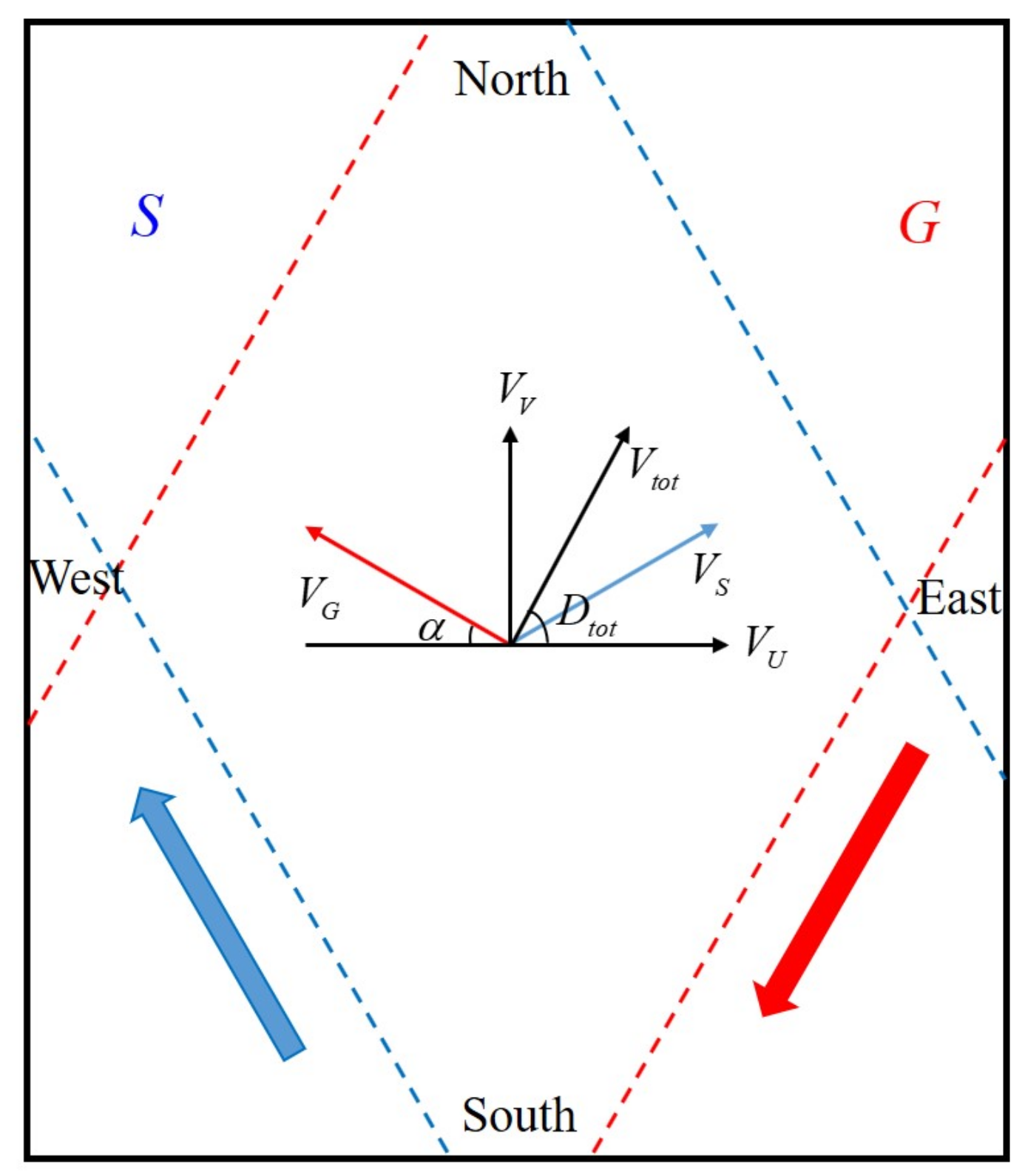
The trajectory-crossing method needs to use two sets of spaceborne SAR data with overlapping areas, usually from ascending and descending passes, respectively, and their acquisition time should be close. Geometric relationships of different velocity components of sea-surface motion over overlapping area are shown in
Figure 1, where the blue and red thick arrows indicate the flight direction of the ascending and descending satellite, respectively. The sea-surface imaging range is
S and
G, bounded by blue and red dashed lines, respectively. The middle is the overlapping area of
S and
G, where
and
represent the magnitude and direction of current velocity, respectively. Sea-surface movement produces projection components in four directions, where
and
represent horizontal radial velocity components along beams far from the ascending and descending satellites.
and
represent surface velocity components along the north–south and east–west directions, respectively. In addition,
represents the intersection angle between the direction of the beam center line and the east–west direction on the horizontal plane.
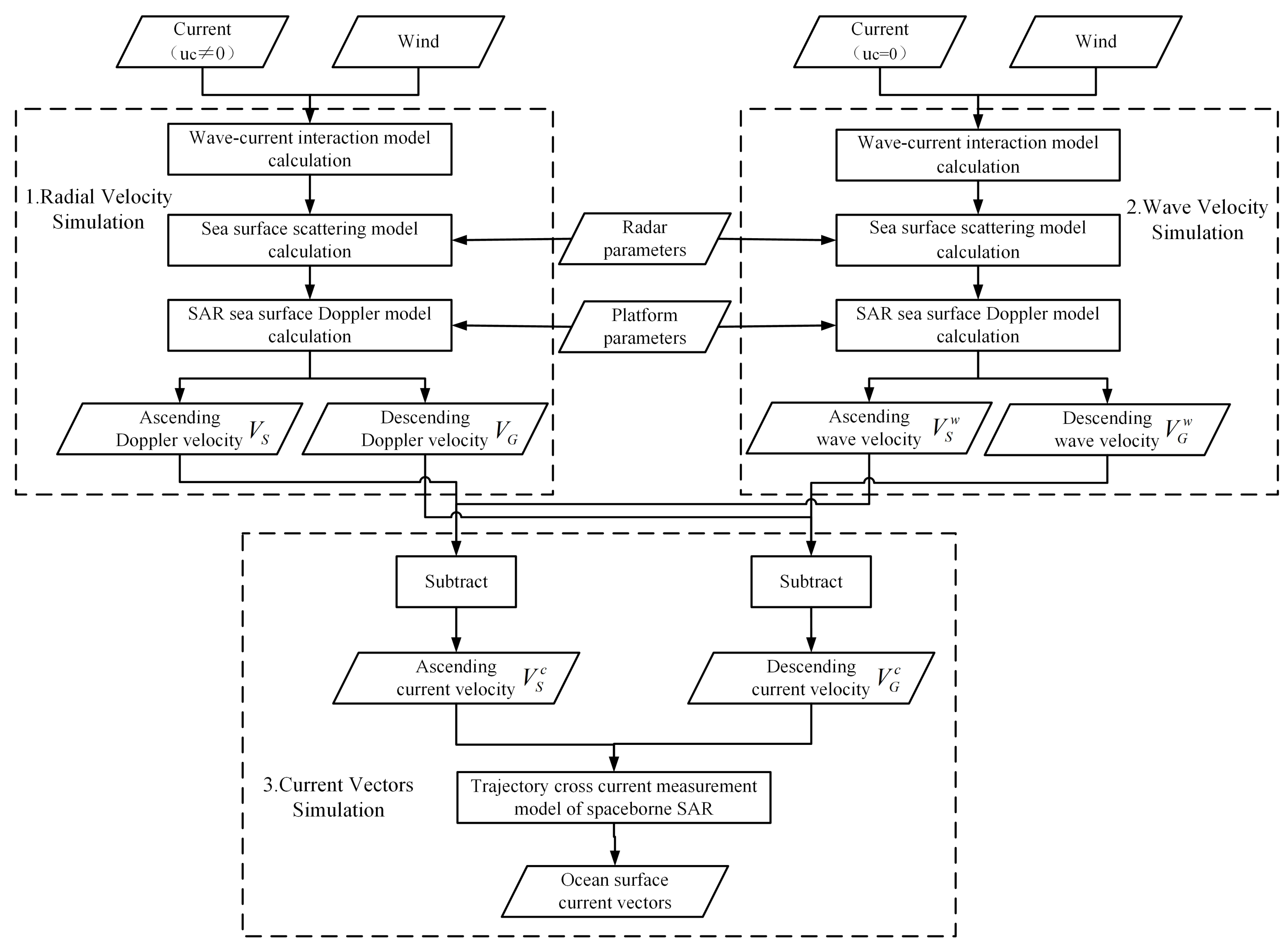
The simulation method proposed in this paper is mainly divided into three parts: radial velocity simulation, wave velocity simulation and current vector simulation. The flow chart is shown in
Figure 2. The first step is to calculate the radial velocity using the SAR ocean imaging model, the second step is to calculate the wave motion component, and the third step is to calculate the two-dimensional current field combined with the trajectory-crossing method. The radar parameters include the signal frequency, look direction of the beam and incident angle. Platform parameters include the satellite orbit height and flight speed.
Based on the SAR ocean imaging model [
7,
8,
9] proposed by Romeiser, University of Hamburg, Germany, the sea-surface horizontal radial velocity components along the spaceborne SAR beam look in directions with the ascending and descending passes simulated. The model supports simulation in the frequency range of 0.4 to 35 GHz. The main processes include the calculation of the wave–current interaction model, sea-surface scattering model and sea-surface SAR Doppler model.
Wave–current interaction is a physical process that must be considered in the real sea motion environment. We need to first give the sea-surface-current field and wind field parameters and then solve the action spectrum balance equation and calculate the modulated wave spectrum according to the weak hydrodynamic interaction theory. The action spectrum balance equation to be solved is [
9,
13,
14]
where
t represents time,
represents the sea-surface spatial position,
represents the wave number, and
and
represent the wave numbers in the X and Y directions, respectively.
N represents the action spectral density of sea-surface micro scale wave,
U represents the surface current field, and
represents the modulated wave group velocity. These variables about ocean waves are related to the conditions of sea-surface wind field.
Q represents the source function:
where
represents the action spectral density in the sea-surface equilibrium state, and
represents the relaxation rate.
The relationship between the wave spectrum and action spectral density is [
15]
where
represents the modulated wave spectrum. The natural angular frequency
,
g is the gravitational acceleration,
is the seawater density, and
is the seawater surface tension.
The sea-surface scattering model is based on the improved combined sea-surface model [
8,
9] proposed by Romeiser and Alpers, which considers the modulation effect of large-scale wave on small-scale Bragg waves. The normalized scattering coefficient can be calculated by taking the modulated wave spectrum and the given radar parameters as the input of the scattering model [
8,
16]
where the symbol
represents the statistical average;
represents the normalized backscattering coefficient when the sea-surface slope is zero;
is the sum of second-order Bragg scattering caused by sea-surface slope;
represents the sea-surface slope vector;
and
, respectively, represent the Bragg wave number components parallel and perpendicular to the radar look direction;
represents the wave number spectrum; ∧ and ∨ denote the Fourier transform and its conjugate of
to wave number
; and
and
denote the Fourier transform and its conjugate of
to combined wave number
.
The Doppler spectrum and variance can be calculated using the double Gaussian Doppler spectrum model [
7] proposed by Romeiser and Thompson, which divides the sea-surface echo into the superposition of the Bragg wave Doppler spectrum far from and towards the radar. Each Doppler spectrum component is defined as a Gaussian shape and expressed as
where ± represents the Bragg wave components away from and towards the radar, respectively;
is the Doppler center weighted by the normalized backscattering coefficient; and
is the variance of Doppler spectrum. The specific calculation formulas of
and
can be found in [
7]. Then, the horizontal Doppler velocity
along the beam radial direction can be expressed as
where
is the wave number of the electromagnetic waves, and
is the incident angle. Therefore, the radial horizontal sea-surface Doppler velocity along the ascending and descending satellite beam represented by
and
in
Figure 2 is calculated successively by the above process.
The radial velocity is actually the Doppler velocity that reflects the average motion state of scatterers in the sea-surface resolution unit. In the range of medium incident angles, the radial Doppler velocity
includes not only the current velocity but also the component of the sea-surface wave motion [
17].
where
is the current velocity,
is the large-scale wave orbital velocity, and
is the net Bragg wave phase velocity.
At present, the related wave motion model is not perfect, and thus it is difficult to extract the current velocity component by directly calculating the accurate wave velocity [
10]. The authors in [
18] stated that when there is no current field, the sea-surface velocity obtained by using the SAR ocean imaging model comes from the wave motion. Therefore, in the second step, the input current field velocity is set to zero, combined with the same wind field, and through the calculation process similar to the radial velocity, the wave motion velocities in the ascending and descending beam direction are obtained, which are
and
, respectively. Since the influence of large-scale waves is considered in the previously used wave spectrum and scattering model, the simulated wave velocities include the sum of the last two velocity components of Equation (
7).
By making a difference between the radial Doppler velocity and the wave velocity, the current velocity components
and
in the ascending and descending beam direction can be obtained:
Then, combined with the trajectory crossing current measurement geometric model in
Figure 1, the east–west velocity component
and north–south velocity component
of the sea-surface current can be calculated:
Finally, the magnitude and direction of the current vector are, respectively, expressed as:
3. Simulation Experiment and Verification
In this section, a simulation experiment was conducted based on the spaceborne SAR system and sea environment parameters. The effectiveness of the simulation method was verified by comparing the simulation results with the measurement results using SAR data. First, the spaceborne SAR data, system parameters and input sea environment data involved in the experiment are introduced. The geographical location of the spaceborne SAR data used in this paper is shown in
Figure 3. This is the Mozambique strait between southeast Africa and Madagascar, where the sea surface is affected by the warm current of Mozambique, and the motion state is relatively stable. The red box indicates the stripmap SAR data range of ESA sentinel-1 satellite’s ascending pass, the acquisition time is 8 October 2019, 15:35 UTC (orbit number: 018385), the black box indicates the stripmap SAR data range of China Gaofen-3 (GF-3) satellite’s descending pass, and the acquisition time is 9 October 2019, 02:43 UTC (orbit number: 016651). Although these two SAR data were not acquired at the same time, the time interval is short, the current motion status is basically unchanged here, and these two SAR images overlap partially in this sea area, which meets the requirements of the trajectory-crossing method.
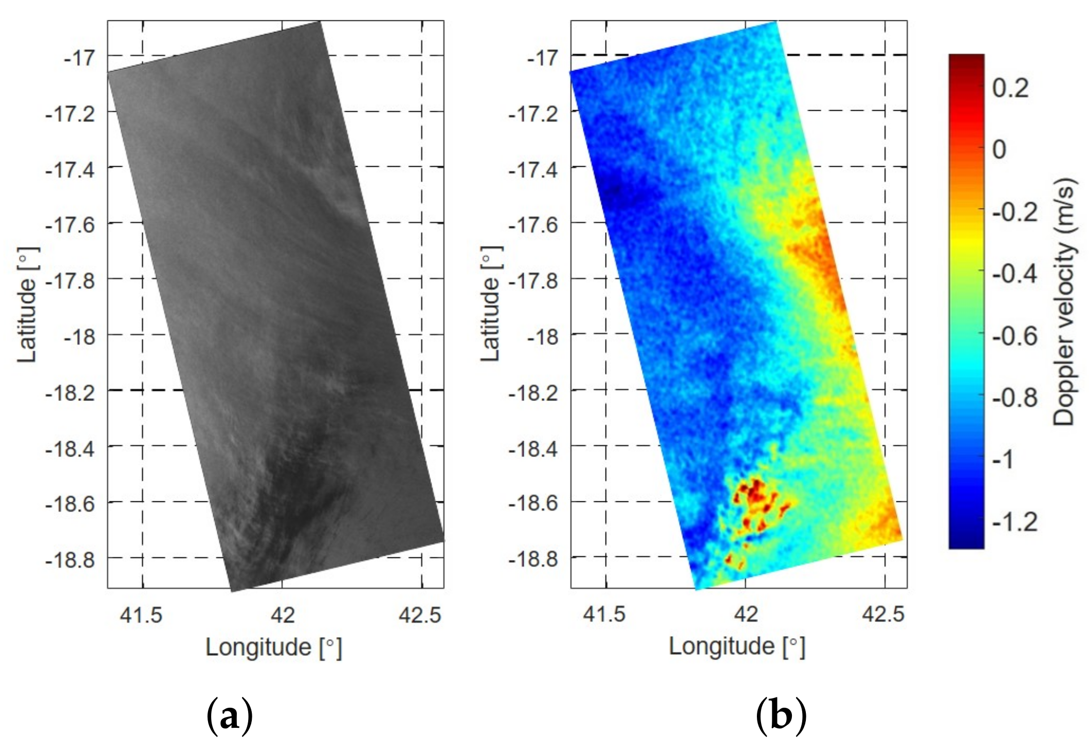
Figure 4 shows the SAR amplitude image of Sentinel-1 satellite and the horizontal radial Doppler velocity image of its secondary product. The dimmer brightness in the lower left corner of
Figure 4a is due to the lower wind speed and the weaker echo energy due to the oil spill on the sea, which also results in errors in the Doppler velocity, as shown in the corresponding position in
Figure 4b. The absolute values are small in the lower right part of the Doppler velocity map, and the overall velocity includes the influence of sea-surface wind and wave motion, which needs to be further removed.
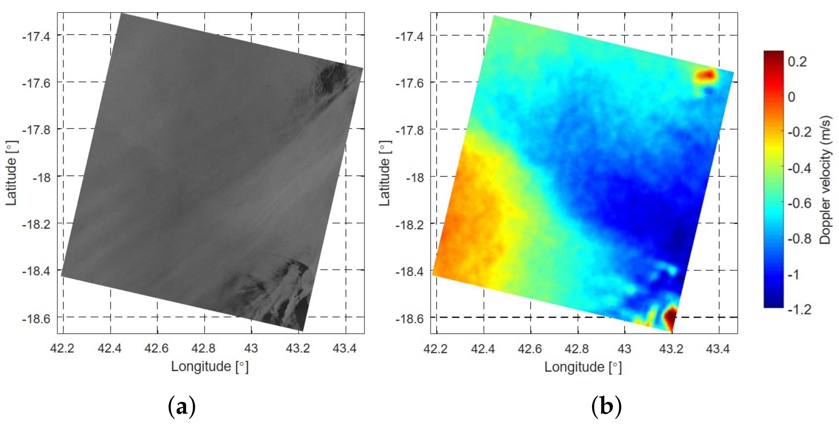
Figure 5 shows the SAR amplitude image of the GF-3 satellite and the Doppler velocity estimated from the single look complex (SLC) data. The dark part of the right corner of
Figure 5a is obviously affected by the sea oil film, which reduces the signal-to-noise ratio of the image. The Doppler velocity of
Figure 5b is estimated from the Doppler processing in reference [
19]. It can be seen that the absolute value in the lower left corner of the image is small, in addition to the anomaly in the oil film position, and the overall velocity overlaps with the influence of the wind and wave motion.
Although the overlap range of the above SAR data is small, it has clear velocity characteristics, which is conducive to the validation of simulation method. Therefore, a simulation experiment was performed in this sea area. The input system parameters are consistent with the real SAR data parameters, representing the ascending Sentinel-1 satellite and the descending GF-3 satellite, respectively, as shown in
Table 1. It should be noted that, at present, there are few ascending and descending data from a single satellite that can meet the requirements of irradiating the same sea area at a short time, and it is difficult to obtain them directly. In future applications, two or more satellites must cooperate to obtain the ascending and descending passes data of the same space-time sea area for current measurement. Therefore, the following dual satellite SAR data processing and system simulation are of practical significance.
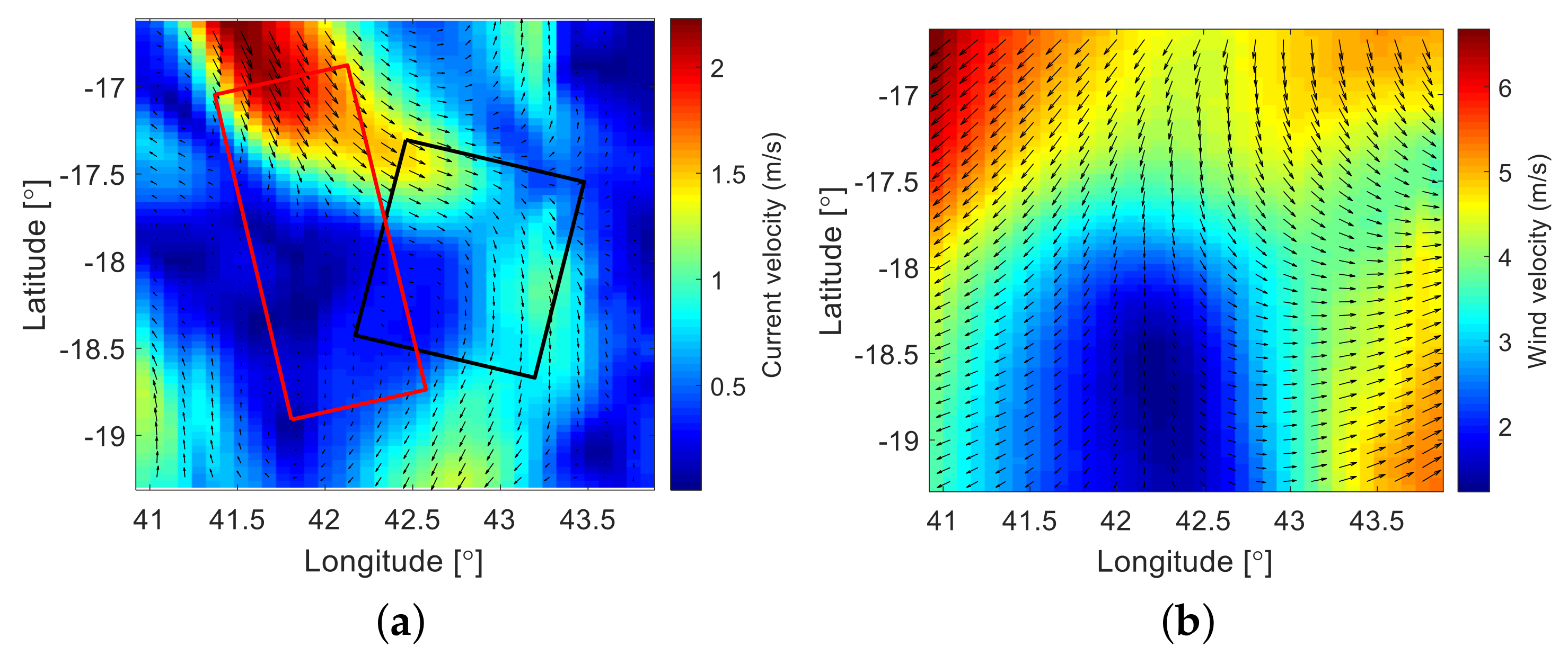
The hybrid coordinate ocean model (HYCOM) reanalysis current field data and the European centre for medium-range weather forecasts (ECMWF) wind field data are obtained for the simulation input, respectively, as shown in
Figure 6. The HYCOM model reanalysis data, which combines satellite altimeter data with temperature and salt data obtained by a buoy, is widely used in ocean current research [
20,
21,
22]. The date selected for the HYCOM data is the same as Sentinel-1 SAR data acquisition date with spatial resolution of 1/12 degree. Wind field data at the same time and place were obtained from the ECMWF website with spatial resolution of 1/4 degree, and interpolated to ensure the same number of data points as the input current field. From the input data, it is known that the velocity in the overlapping area is small, and the sea-surface wind speed is mainly in the range of 2–7 m/s, which belongs to the moderate wind speed.
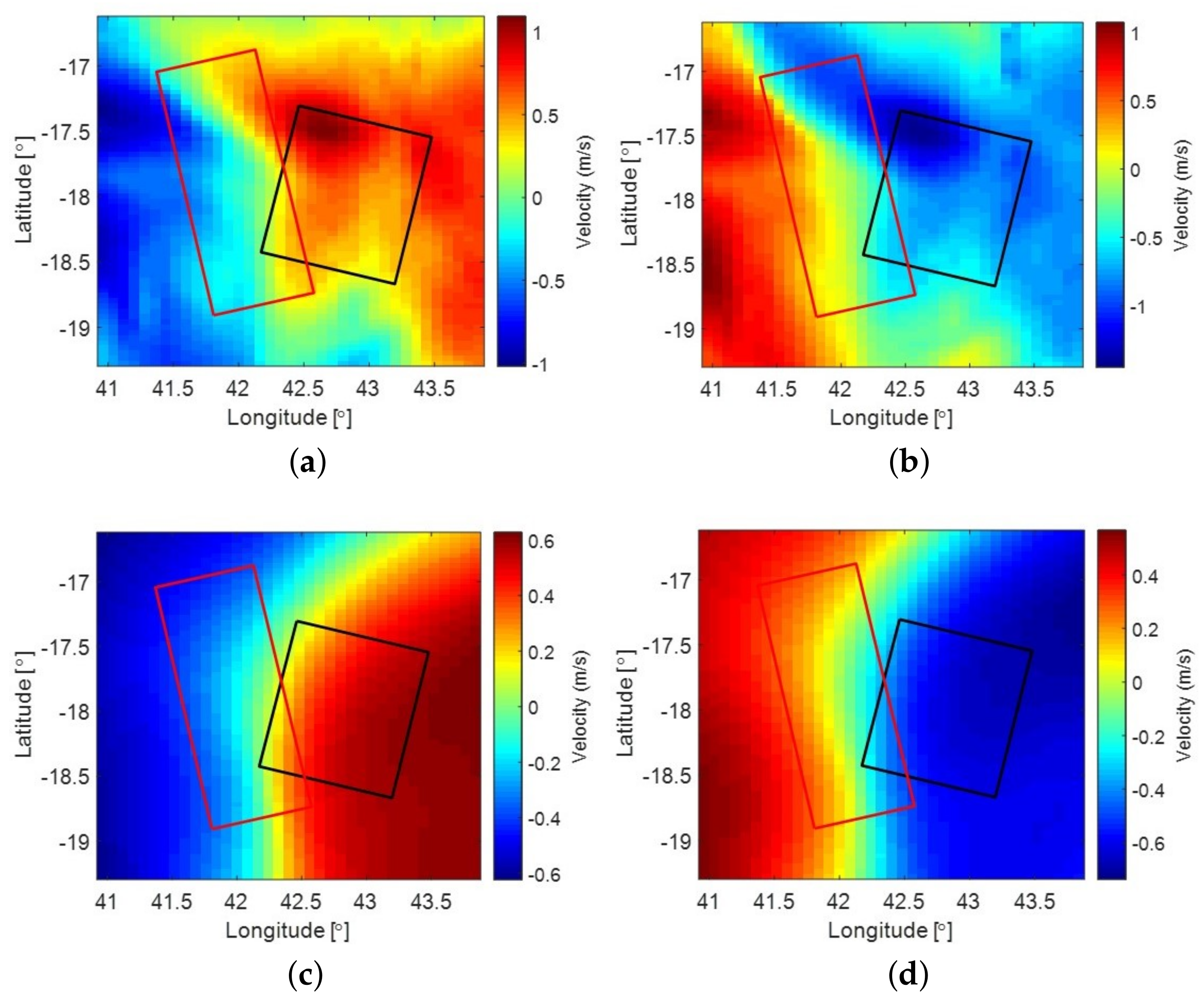
The given current and wind data are input into the SAR ocean imaging model to calculate the radial Doppler velocity
under the parameters of ascending Sentinel-1 satellite and the radial Doppler velocity
under the parameters of descending GF-3 satellite, as shown in
Figure 7a,b, respectively. It can be seen that, due to the same orbital inclination of these two satellites, the distribution of the relative value of the velocity in the look direction of the two beams is approximately symmetrical; however, the absolute value is different due to the influence of wind and wave motion.
Figure 7c,d shows the wave velocity when the current field is set to zero under the same wind field conditions, in which the absolute value of the velocity changes due to the change of the relationship between wind direction and beam look direction. When the wind direction is perpendicular to the beam look direction, the wave velocity is zero, which is consistent with the research conclusion in the literature [
11].
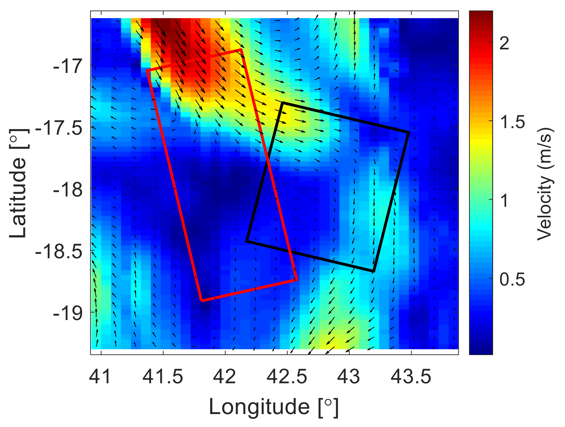
According to the flow chart in
Figure 2, the corresponding sea-surface radial velocity and wave velocity of ascending and descending passes in
Figure 8 are subtracted, and the current vectors are calculated using the trajectory-crossing method. The simulated two-dimensional current field is shown in
Figure 8. Comparing with the input current field given in
Figure 6a, we found that they were in good agreement. Note that, as for the computational demand, the calculation process of this method takes only a few minutes, the calculation amount of wave spectrum is the largest. The calculation times will be different according to the amount of input current and wind data.
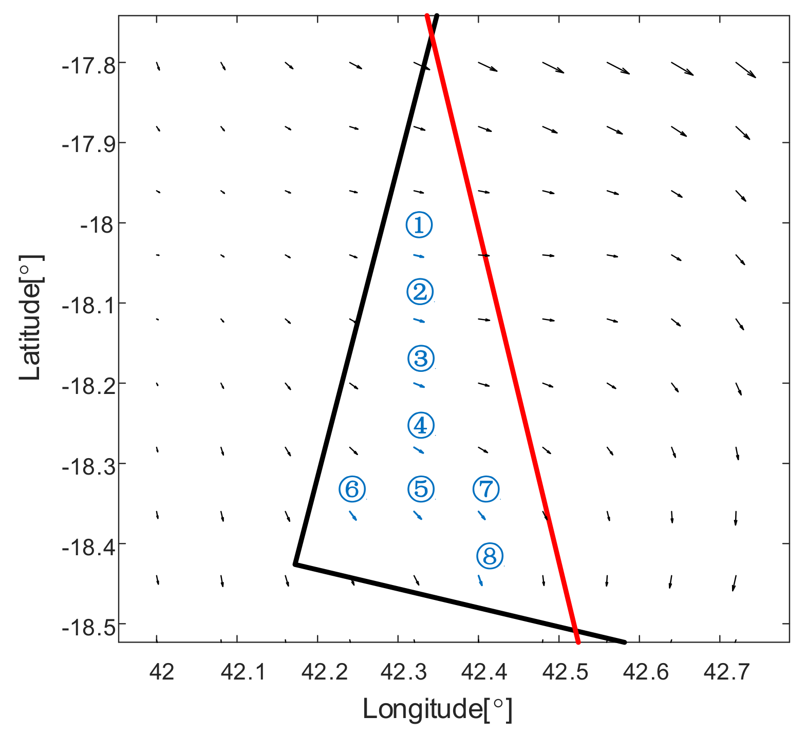
To quantitatively validate the experimental results, we selected eight geographic locations in the overlap area (
Figure 9) and compare the simulation results with the SAR data measurement results, as shown in
Table 2. As the size of the simulated current field resolution unit is about 8 km and that estimated from Sentinel-1 and GF-3 SAR data is about 1 km, the 8 × 8 Doppler velocities around the corresponding eight latitude and longitude positions in
Figure 4b and
Figure 5b are averaged. After subtracting the simulated wave velocity in
Figure 7 from the average data, the two-dimensional current field results of the SAR data are calculated in combination with Equations (8)–(13). It can be seen that the corresponding current velocity and direction are close. However, because the current and wind data input by the simulation will be different from the instantaneous environment in the real SAR data, there will also be discrepancies between the data in
Table 2.
The statistical analysis of the experimental data is shown in
Figure 10.
Figure 10a shows a scatterplot of the velocity of the simulated current field compared with that of the measured current field from SAR data, with a correlation coefficient greater than 0.9 and a root mean square error (RMSE) of 0.028 m/s.
Figure 10b shows the scatterplot comparing the direction of the simulated current compared with that of the measurement data. The correlation coefficient is greater than 0.98 and the root mean square error (RMSE) is 6.05 degrees. It can be seen that the simulated current field is in good agreement with the measured current of SAR data.
We also notice that there is a visible deviation between these two data, which will not only come from the difference of input data but also be limited by the model. For example, the wave spectrum is different from the real sea-surface state. Nevertheless, we believe that the simulation results are consistent with the measurement results. Therefore, the proposed method in this paper can effectively simulate the two-dimensional sea-surface-current field in the given spaceborne SAR system and marine environment parameters. The results also show that the proposed simulation method is conducive to the parameter analysis process of the trajectory-crossing method in the application of current measurement in the future.


