SSA-CAE-Based Abnormal Data Classification Method in Edge Intelligence Device of CNC Machine

Abstract

Smart factories and big data are important factors in the Fourth Industrial Revolution. Smart factories aim for automation and integration; however, the most important part is the application of data. Despite extensive research on the maintenance and quality management of big data-based production equipment, industrial data gathered for analysis contain more normal data than abnormal data. In addition, a significant amount of energy is expended in the data pre-processing process to analyze the acquired data. Therefore, to maintain production equipment and quality management, data classification technology that allows easy data analysis by classifying abnormal data into normal data is required. In this paper, we propose an abnormal data classification architecture for cycle data sets gathered from production facilities through SSA-CAE along with data storage methods for each product unit. SSA-CAE is a hybrid technique that combines singular spectrum analysis (SSA) techniques that are effective in reducing noise in time series data with convolutional auto encoder (CAE) that have performed well in time series.

1. Introduction

Since the 4th Industrial Revolution, the smartization of the manufacturing industry using information and knowledge has been rapidly growing. Computer numerical control (CNC) [1], machining center tool (MCT), and injection molding machines are typical production equipment applied to smart factories. Various sensors are installed and operated in the factory for detecting defects and maintaining the production facility. It is possible to build a monitoring system using data gathered from sensors. Sensors are used for predictive preservation of production machines, optimization of manufacturing processes, and real-time abnormality detection using applying data analysis [2], machine learning [3,4,5,6] and deep learning [7,8,9] technology. According to these changes, various research studies have been conducted in academia based on sensor data. Data collected from the sensor data [10,11,12,13,14] are stacked up as big data and stored in a data center at the manufacturing site or in a cloud environment. Owing to the rapidly growing computing power the analyze of big data has recently been in the spotlight.

However, there is a fatal problem with sensor data gathered from manufacturing facilities. The state of big data from most of the manufacturing facilities is more imbalanced than that of normal data. Furthermore, it is not easy to gather abnormal data unless the equipment intentionally fails because the tools are replaced periodically based on the experience of expert workers.

To solve the class imbalance of data, research studies have been conducted to detect outliers in data by learning only normal data. However, previous studies have focused on the correlation between the time of occurrence of the abnormality in all data, and the reasons of the abnormality. To detect abnormalities in CNC machines, the most representative machine tools in the manufacturing industry, have various data such as physical properties information of raw materials, vibration of motors, and discharge of lubricants. These data are applied as elements of abnormal detection [15,16]. Owing to the nature of the time series, data is continuously gathered and stored by time. Most big data processed for analysis after storage, consumes considerable time and effort to pre-process time series data. Therefore, the detection of abnormalities in the product unit takes precedence before focusing data on abnormalities and factors that affect their occurrence. In this study, class imbalance was resolved and approached as a computing architecture for data storage methods and data classification. This study focused on product-level collection and analysis, data-oriented collection, and analysis. In addition, we aim to detect the problem state, which is abnormality, during processing of each single product, not to classification the reason of processing problem state.

The data used in this study utilizes sensor data collected by CNC. Many studies have been conducted on abnormality detection for CNC predictive preservation [17,18]. However, related studies have only performed abnormality detection for the entire collected data. To apply it to the real field, product-oriented data storage and abnormality detection are required rather than, the entire data. The contributions of the study are as follows: A new architecture using the SSA [19] technique and the unsupervised deep learning model [20] is proposed. It also increases the usability of big data collected from smart factories through new proposals on how to store data.

The validity of the storage and analysis methods of CNC data is verified through experiments. It also applies and compares various proposed techniques to improve class imbalance and demonstrates the performance of the proposed classification model. In addition, an experiment was conducted to confirm the effectiveness of the proposed architecture to determine whether the architecture could record valid performance when applied in practice. The experiment was conducted based on sensor data collected at the real site and utilized vibration data from the CNC machine. After the experiment, the characteristics of the proposed architecture and considering it, areas that are good to be applied.

Our contributions through this paper are as follows.

• For the smartization of small and medium-sized manufacturing industries that are do not have the latest facilities, we propose an architecture for data collection methods and classification.
• A deep learning classification technique based on the SSA technique is proposed.
• Through the proposed classification technique, “product with data” can be achieved within a smart factory.

“Product with data” refers to a group of data generated in product units, not data collected for one day or data for each process unit. The composition of this paper is as follows. First, Section 2 describes previous studies. Recent research trends and previous related studies are presented along with abnormal detection studies using CNC data, problems of class imbalance data, and previous studies to solve them. Section 3 introduces the configuration of the data classification architecture to be proposed in this paper. Along with the overall structure, the expected effects of the detailed components of each structure are introduced in detail. Section 4 presents the results of the applicability and experiments on the propositions to be proven in this study. Finally, Section 5 summarizes the contents of the thesis, introduces future research, and concludes the thesis.

2. Related Work

2.1. Smart Factory and Big Data

Automation production facilities associated with smart factories contain numerous sensors, and diverse data are collected through programmable logic controller (PLC). Some data are used for data analysis, however, there are also highly volatile data such as information displayed on indicators installed in production facilities. When the torque overload caused by over-insertion of the machine instrument exceeds the threshold, you will be notified, and the machine view of the defect assessment and load cell installed on the conveyor will also operate offline. Various values can be generated by accumulating processing analysis in real time only with data that is instantly discarded. If a typical big data analysis is the process of finding meaningful things by applying various algorithms to vast amounts of data accumulated over a long period of time is a common big data analysis [21], smart factory data processing focuses on notifying production sites of more real-time analysis [22]. Analog data such as temperature, humidity, concentration, pressure, and weight are directly or indirectly related to product quality maintenance and can reduce costs through mutual correlation analysis. Machine facilities can be predicted and preserved through analysis techniques such as machine learning and AI algorithms, which provide important data for maintenance cost and energy saving, using data such as facility load patterns and vibration frequencies of existing sensors. For this data analysis, it is necessary to focus on the quality of the collected data. It is not a big data analysis method that accumulates and analyzes data, but a data state generated when collecting data in real time. Only then can the value of data used in smart factories be increase.

2.2. CNC Machine

CNC machines are widely used in manufacturing facilities to manufacture products according to the desired shape and conditions by entering predefined commands [23]. The operating principle of CNC begins with direct coding through a CNC machine or PC with a CNC programming application. The program or order transmitted and executed to the CNC machine performs the process according to the program and the desired form. Depending on the process, various methods are used, and the types of data collected are different. The collected data is representative of vibration, temperature, speed, power, current, and noise. Various research studies have been conducted to detect abnormalities in the mechanical system of CNC machines. According to previous studies, vibration, power, and noise data are typical data used to prove the cause of failure of CNC machines. A previous researches using motor vibration data of production facilities proposed a technique to solve the imbalance from collected data and detect outliers based on the encoder-decoder-encoder generator based on the generative adversarial network (GAN) model [18].

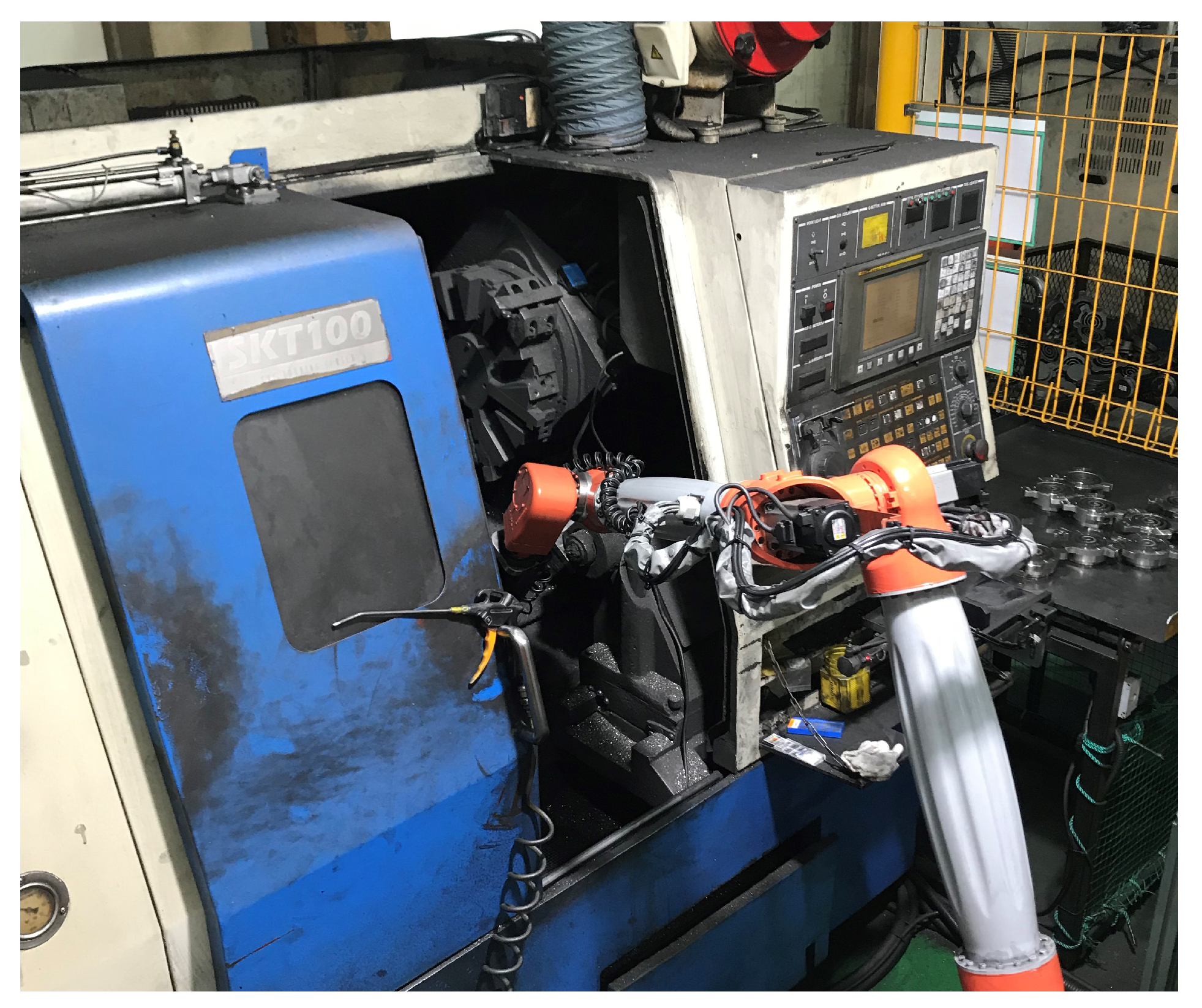
Figure 1 is an actual picture of the CNC machine at the field site where actual data were collected. Two-way processing is performed on this machine. The way of machining that roughly processes the surface is rough machining and fine machining to match the calculated dimensions.In this study, vibration data generated during process are used as a bundle of all machining.

2.3. Edge Intelligence

Edge Intelligence (EI) is a concept that defines the communication, computing, and storage capabilities of a specific infrastructure closest to the local unit user of a distributed network. Previous studies introduced the word “Edge Intelligence” [24]. “Edge” is an actual location representation in which data is generated and processed. In other words, the edge is the location of the control and computing devices. According to a recent study, devices equipped with small computers are changing to internet of things (IoT) and industrial internet of things (IIoT). These devices work with the addition of AI functions. Edge Intelligence performs edge computing in the analysis performed on AI and ML models. The intelligent edge generally breaks the existing client-server model, and the server has the ability to process, analyze, and protect data [25]. Edge Intelligence has three main entities: connection, computing, and control [26]. This Edge Intelligence allows manufacturing systems to refine and classify data to the cloud without additional connections. In addition, Edge Intelligence Devices (EID) interconnect a range of workers, managers, smart facilities, robots, and sensors, and enables extensive connections such as smart factories. Hyper-connected Edge Intelligence systems can collect, manage, analyze, and store large amounts of data through distributed computing. This local computing unit can be combined with a cloud system to improve or replace computing performance. Edge computing is mainly performed by a data collector in a production facility or by an edge server (or IIoT gateway). This feature applies to specific business services that require control of the insights calculated by these local units and may extend to the cloud.

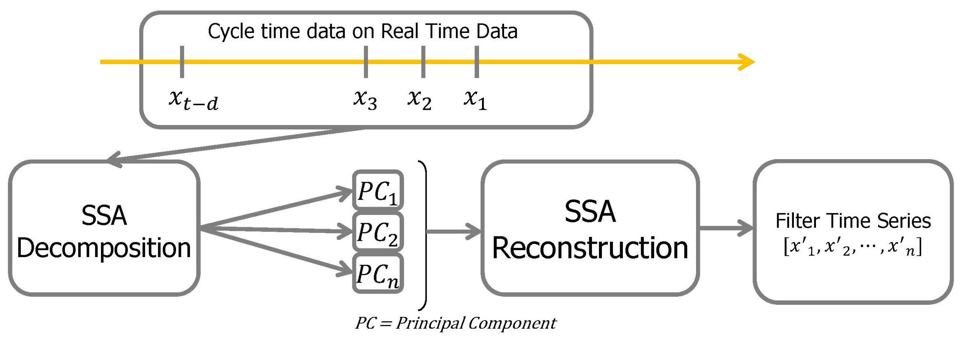
2.4. Singular Spectrum Analysis

SSA is a time series analysis and prediction technique. Based on Karhunen-Loeve transformation theory, this technique combines classical time series analysis, multivariate statistics, multivariate geometry, dynamic systems, and signal processing elements. SSA aims to decompose the original series into a slow-changing trend, component decomposition such as vibration components, and the sum of a few interpretable components such as noise. This is based on the singular value decomposition (SVD) of a specific matrix configured on the time series [27,28,29]. Components with vibration are first extracted, and then meaningful components are selected for reconstruction. In summary, the algorithm consists of embedding, single value decomposition, grouping, and reconstruction.The process of SSA, the data is rearranged by decomposing the input data into principal components (PCs) and grouping PCs. This process briefly shown in Figure 2.

2.4.1. Embedding

The first step of SSA is to map time series data F to a multidimensional delay vector [28,30]. The integer value L is set to the window length, which is $2\le L\le \frac{N}{2}$. When $i=0,\cdots ,N-L$, the window length is obtained by the sub-series $\left\{f_i,f_{i+1},\cdots ,f_{i+L-1}\right\}$. This window moves along the time series, forming a column vector $X_i$ for each sub-column. $X_i$ is defined as follows.

$$\begin{array}{cc}\hfill & X_0={\left(f_0,f_1,f_2,\cdots ,f_{L-1}\right)}^T\hfill \\ \hfill & X_1={\left(f_1,f_2,f_3,\cdots ,f_L\right)}^T\hfill \\ \hfill & X_2={\left(f_2,f_3,f_4,\cdots ,f_L\right)}^T\hfill \\ \hfill & X_3={\left(f_3,f_4,f_5,\cdots ,f_L\right)}^T\hfill \\ \hfill & ⋮\hfill \\ \hfill & X_{N-L}={\left(f_{N-L},f_{N-L+1},f_{N-L+2},\cdots ,f_{N-1}\right)}^T\hfill \end{array}$$

(1)

For Equation (1), the vector of each row forms an L-trajectory matrix, a time series of $X_i$. The matrix formed is as follows. This matrix is called the Hankel matrix.

$$X=\left[\begin{array}{cccccc}{f}_0& f_1& f_2& f_3& \cdots & f_{N-L}\\ f_1& f_2& f_3& f_4& \cdots & f_{N-L+1}\\ f_2& f_3& f_4& f_5& \cdots & f_{N-L+2}\\ ⋮& ⋮& ⋮& ⋮& \ddots & ⋮\\ f_{L-1}& f_N& f_{L+1}& f_{L+2}& \cdots & f_{N-1}\end{array}\right]$$

(2)

$K=N-L+1$ represents the number of columns of the trajectory matrix, the column of X is called the L-lagged vector, and the row is called the K-lagged vector.

2.4.2. Decomposition

The second step in SSA is decomposition. The Trajectory matrix is decomposed using SVD. It is classified into three categories that constitute X. U is the unit matrix of $L\times L$ containing the left-specific vector orthogonal set of X as a column. $\mathrm{\Sigma }$ is an $L\times K$ rectangular diagonal matrix containing an X value of L, and is aligned with the largest and smallest values. Finally, V in Equation (3) is a $K\times K$ unit matrix including an orthogonal set of right-specific vectors of X. The equation for X is as follows:

$$X=U\mathrm{\Sigma }{V}^T$$

(3)

Using a SVD equation for the Trajectory matrix is expressed as follows:

$$\begin{array}{cc}\hfill & X=\sum _{i=0}^{d-1}{\sigma }_i{U}_i{V}_i^T\hfill \\ \hfill & \equiv \sum _{i=0}^{d-1}{X}_i\hfill \end{array}$$

(4)

Here, ${\sigma }_i$ represents to the i-th singular value, and $U_i$ and $V_i$ are vectors representing the i-th column of U and V, respectively. $d\le L$ is the rank of the trajectory matrix. It is the i-th elementary matrix. $U_i$, ${\sigma }_i$ and V_i denotes the i-th eigentriple of the SVD.

2.4.3. Grouping and Reconstruction

Because the time series is uniquely determined in the Hankel matrix, the equation below defines time series F as the sum of the components $\widetilde{F_i}$. After grouping these components and classifying them into trends, periodicity, or noise. The equation for grouping is as follows:

$$X=\sum _{i=0}^{d-1}\widetilde{X_i}$$

(5)

2.5. Autoencoder

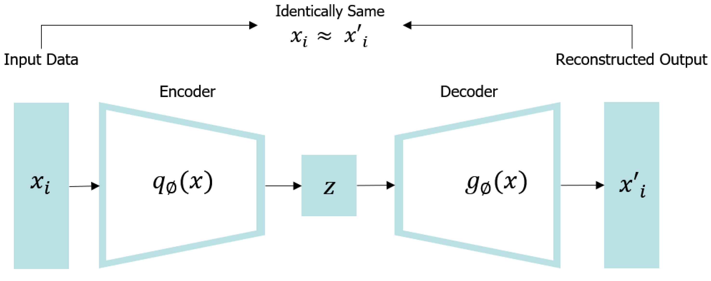
An autoencoder [31] is a neural network that compares input and output as shown in Figure 3. It makes it a difficult neural network by limiting the network in many ways. For example, the number of neurons in the hidden layer is smaller than that of the input layer, thereby compressing (reducing) data. There are various types of autoencoders, and there is also a model that learns a network to restore the original input after adding noise to the input data. Because the under complete autoencoder cannot copy the input into the output as it is by a low-dimensional hidden layer, the output must learn to include some details from the input. Through this learning, the under complete autoencoder allows to learn the most important characteristics from input data. These constraints prevent the autoencoder from simply copying the input directly into the output and allow it to learn how to efficiently regenerate data.

The encoder, also referred to as a cognitive network, converts an input into an internal expression. The decoder, also referred to as a generative network, converts an internal expression into an output. The encoding operation maps the input data $x_i$ to and the decoding operation reconstructs the input at the latent layer z. It may appear impractical to simply reconstruct input data, however, practical useful characteristics can be obtained by applying some restrictions to autoencoders to obtain $x_i^{\prime }$ so that input data can only be approximate.

In the encoding step, a hidden layer representation of the mapping $q_{\theta }\left(x\right)$ for a given input data set x can be obtained, and the details are as follows.

$$z=q_{\theta }\left(x\right)=S(Wx+b)$$

(6)

In the decoding step, the output data $x_i^{\prime }$ can be reconstructed using the $g_{\theta }\left(z\right)$ function for the hidden layer, and the specific expression is as follows:

$$x^{\prime }=g_{\theta }\left(z\right)=S(W^{\prime }z+b^{\prime })$$

(7)

Here, S is the activation function, $\theta =W,b$ is the parameter set of the encoder, and ${\theta }^{\prime }=W^{\prime },b^{\prime }$ is the parameter set of the decoder. In addition, autoencoder completes learning by minimizing the reconstruction error $L(z,g_{\theta }\left(x\right))$ between $x_i$ and $x_i^{\prime }$.

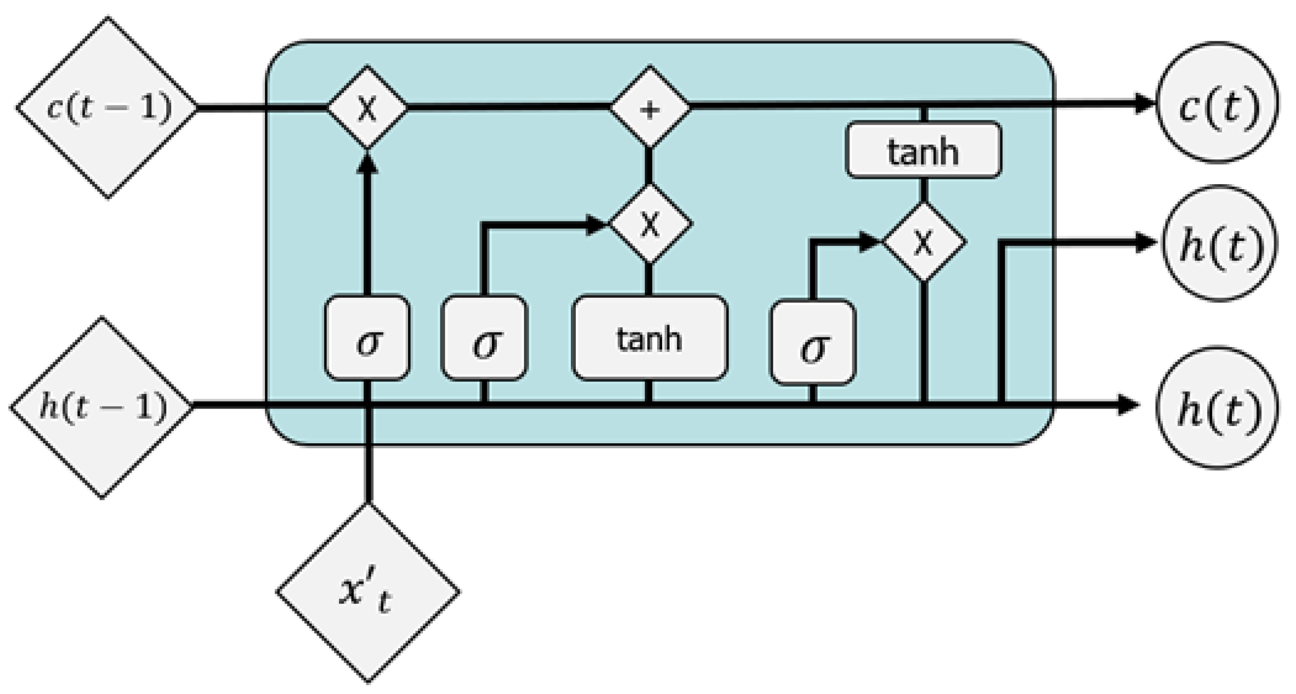
2.6. Long Short-Term Memory

Long short-term memory (LSTM) is a special type of RNN and can perform learning that must have a long dependence period. This model was introduced by Hochreiter and Schmidhuber (1997). All RNNs have the same form as chains that repeat the natural network module. The loop uses the same network repeatedly but allows information to be transferred to different stages. RNN is useful for delivering previous information to the current node, however, one disadvantage is that learning is not smooth when using old historical information. In a basic RNN, this repeated module has a very simple structure. For example, one layer of tanh layer is mentioned. LSTM has the same chain-like structure, but each repeating module has a different structure. Rather than a simple natural network layer, four layers are designed to exchange information with each other in a special way.

The inability to reflect past events in the network was a major drawback of the existing neural network. LSTM that improves these shortcomings. LSTM may effectively model time series data [32,33]. Although it is impossible for existing RNNs to learn from the distant past, LSTM can learn from past events and process both high-frequency and low-frequency signals. The advantage of LSTM is that it shows excellent performance in time series data processing. In addition, the information transfer of the previous cell, which is one in the RNN, is added to the output, enabling short-term and long-term memory. This efficient process briefly shown in Figure 4.

W denotes a weight for connecting the input to the LSTM cell, and $x_t$ denotes a vector input for the current time point t. U represents a weight connecting the previous memory cell state with the LSTM cell, P represents a diagonal weight matrix, T represents $tanh$ non-linearity, and b represents a deflection value. The relevant expressions and main architectures are shown below.

$$\begin{array}{cc}\hfill & i_t=\sigma (W_{{}_i{X}_t^{\prime }}+U_{{}_i{h}_{t-1}}+P_{{}_i{C}_{t-1}}+b)\hfill \\ \hfill & \\ \hfill & f_t=\sigma (W_{{}_f{X}_t^{\prime }}+U_{{}_f{h}_{t-1}}+P_{{}_f{C}_{t-1}}+b_f)\hfill \\ \hfill & \\ \hfill & o_t=\sigma (W_{{}_o{X}_t^{\prime }}+U_{{}_o{h}_{t-1}}+P_{{}_o{C}_t}+b_o)\hfill \\ \hfill & \\ \hfill & c_t=f_t\otimes c_{t-1}+i_t\otimes T(W_{{}_c{X}_t}+U_{{}_c{h}_{t-1}+b_c})\hfill \\ \hfill & \\ \hfill & h_t=o_t\otimes T\left(c_t\right)\hfill \end{array}$$

(8)

3. SSA-CAE Based Abnormal Data Classification Techniques in Edge Intelligence Device

3.1. Architecture of SSA-CAE Based Abnormal Data Classification Techniques in Edge Intelligence Device

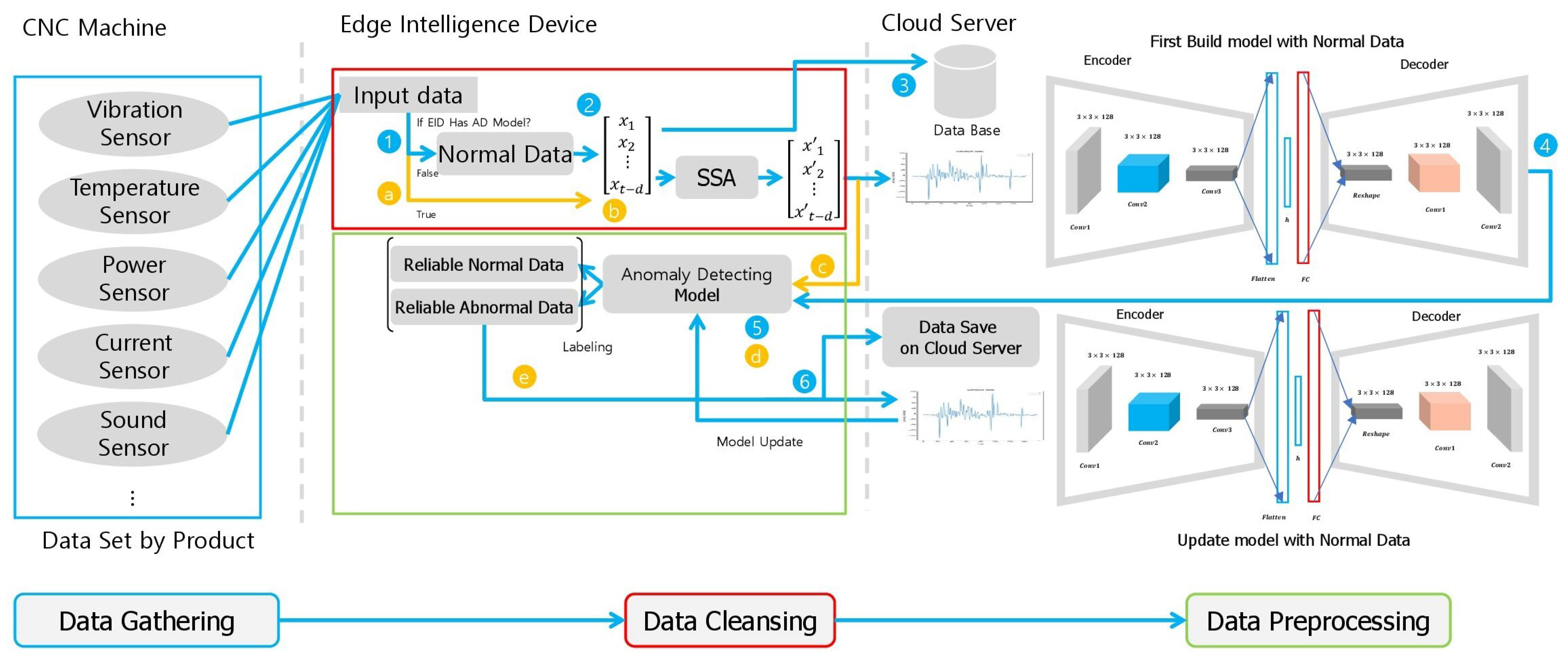
In this paper, we propose a data classification method using the SSA technique and a deep learning technique that is an effective data storage method for data analysis. The structure of the proposed architecture is divided into two spaces in computing space and, with a total of three spaces.

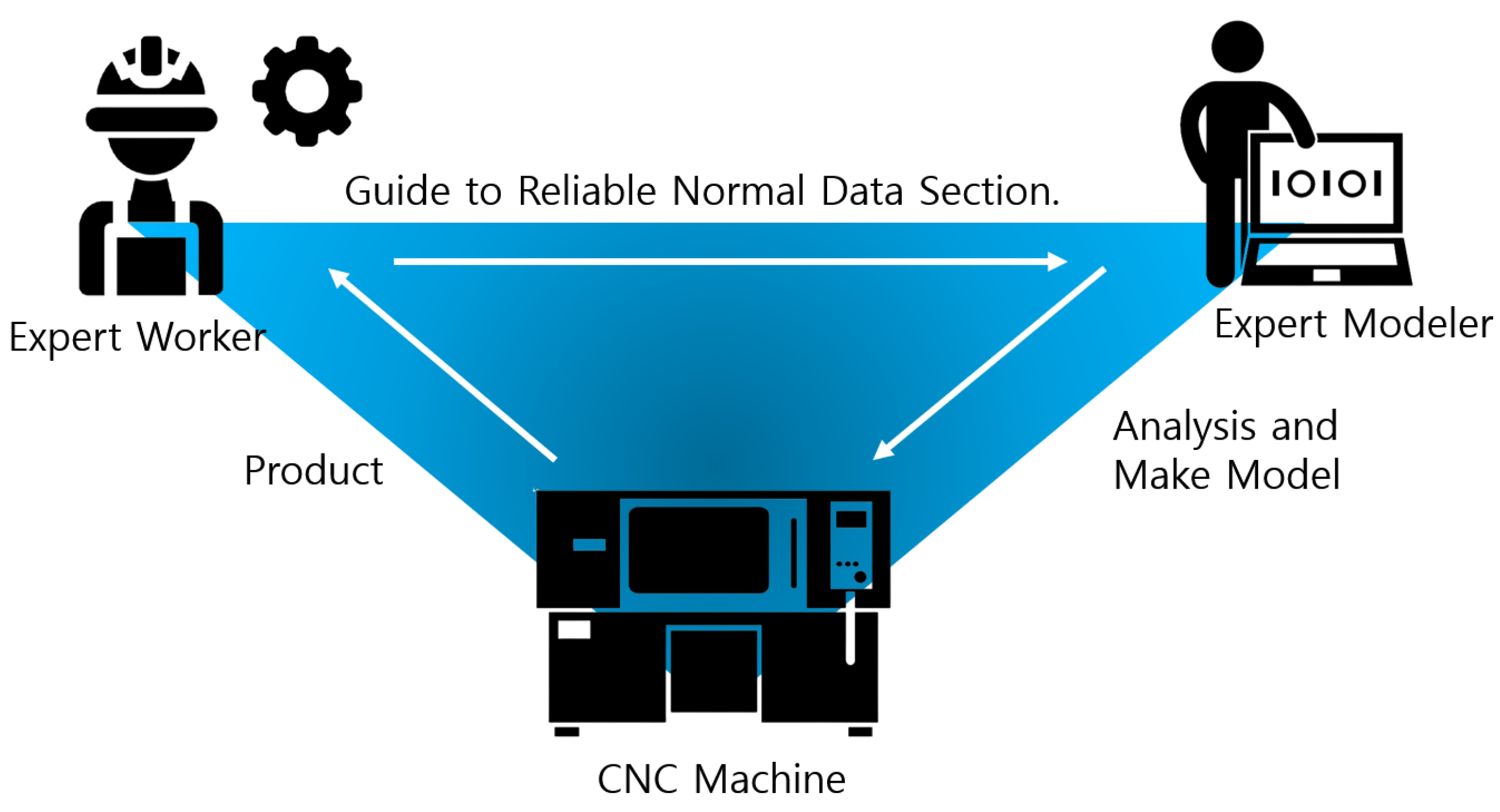
The structure of the entire architecture can be observed in Figure 5. The space where CNC machine and EID are installed is defined as edge computing space, and cloud server is defined as cloud computing space. Data is collected from the PLC or through sensors directly connected to the Edge Intelligence Device. When collecting data, Edge Intelligence Device receives the CNC machine’s work end point from the PLC and obtains calculates a difference between the previous end point and the most recent end point. Time series data collected by each sensor is sliced into product units by matching the start and end time of the collected time series data. This sliced data is divided into raw data and data processed with the singular spectrum algorithm and stored in the cloud. To create a classification model only with normal data, information on the normal section suitable for the judgment of field expert worker deliver to the modeler.

The judgment of field experts is based on the know-how on the number of processing of CNC machines. In this paper, data based on the judgment of field experts are defined as reliable normal data because one worker is not placed in one machine in the field and the criteria for determining the normal state are different for each worker.

The modeling operator performs deep learning modeling based on processing data stored in the cloud. The created model is stored in the form of an API in the EID in the cloud, and the stored classification model distinguishes the normal state and abnormal state of data for each product unit. The normal data classification process and the modeling process required for modeling are briefly shown in Figure 6.

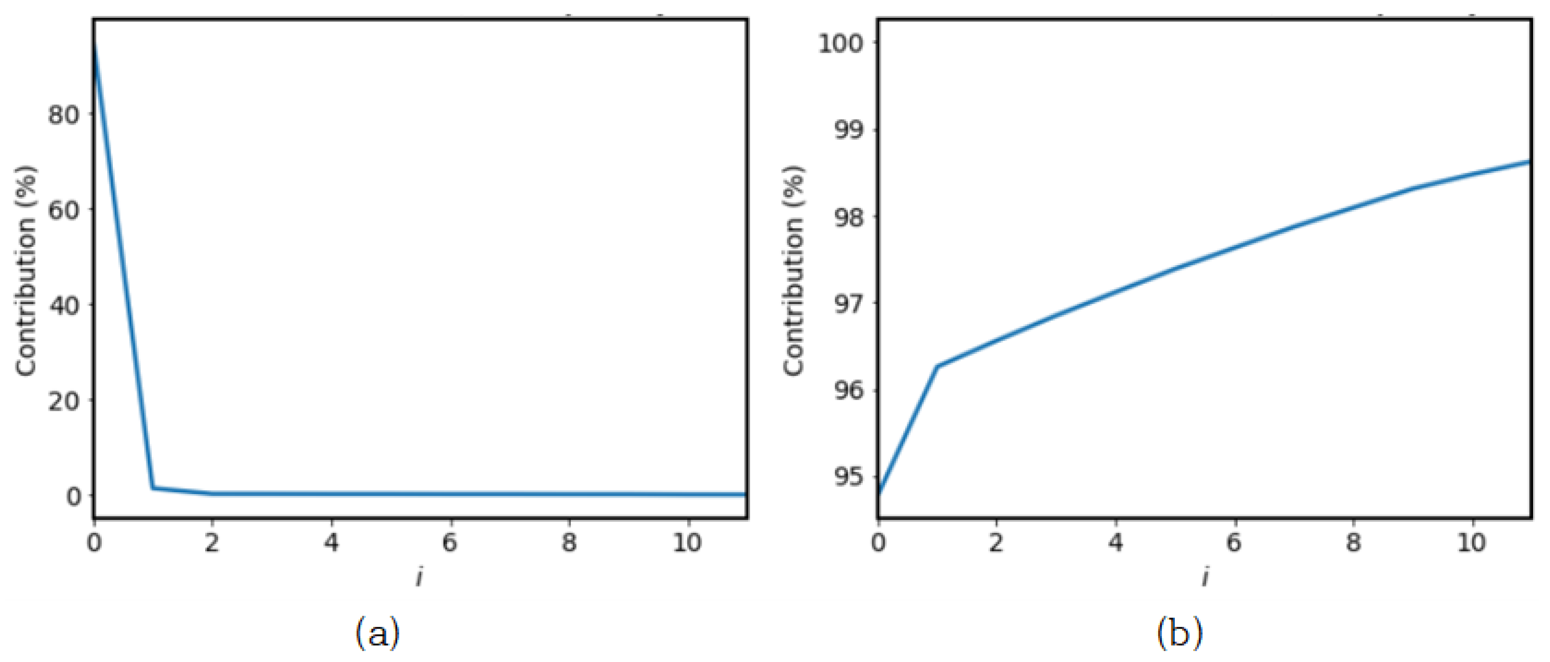
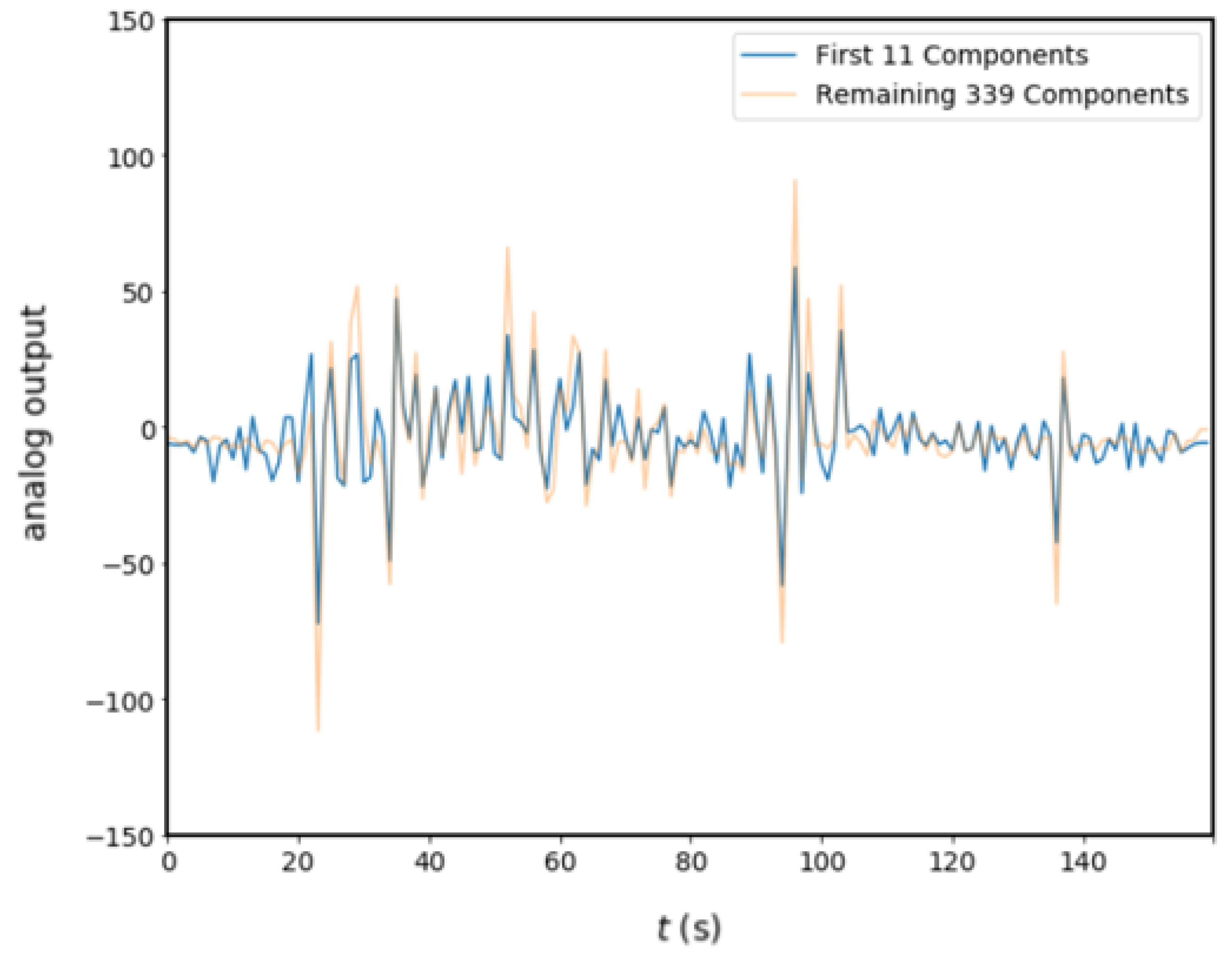
3.2. Data Reconstruction Using Singular Spectrum Analysis

As discussed in previous studies, SSA can be reclassified and reconstructed by decomposing the characteristics of data. It is impossible to apply all types of data generated within the smart factory. Processing data using vision sensors is not suitable for utilization purposes. In addition, if multivariate data are processed at the same time, this analysis technique will be inapplicable.

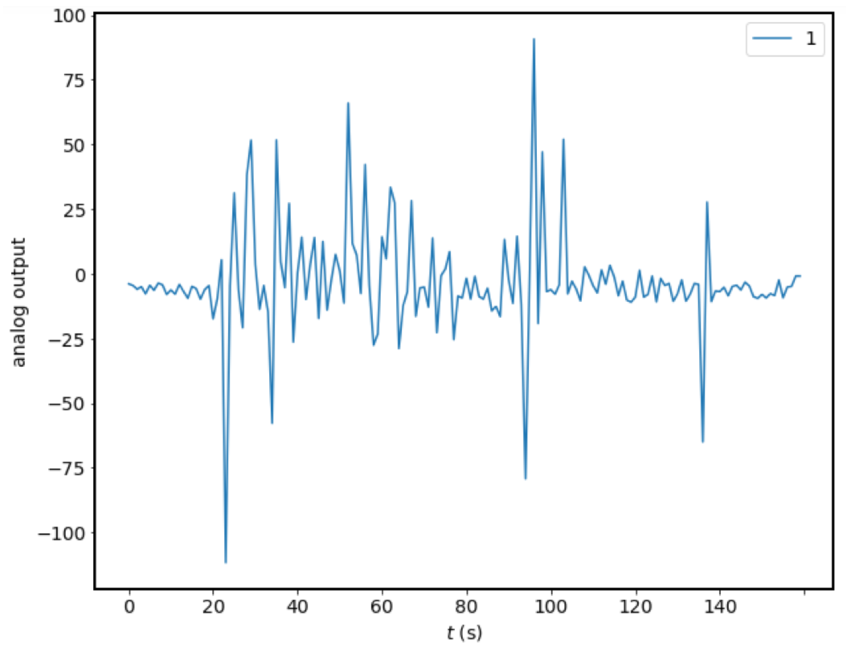
Therefore, this paper focuses on data of one type of data collected in units of products. In Section 4, the experiment was conducted using vibration data. The role of SSA in the proposed architecture is to reduce noise in data collected in the field and to improve modeling performance through periodic component extraction and reconstruction.

Owing to the different characteristics of analog data such as vibration data and voice data, data experts for each data type should analyze the SVD status and input reconstruction information for key components based on the data processed by EID. In general, it is decomposed into trends, predicted values, and noise values of data through the main components generated in the embedding stage of the Singular Spectrum. The rest of the trends and predictions except for noise values are reclassified and reconstructed into noise-reduced data to help the deep learning model analyze actual abnormal values.

3.3. Data Classification Method through Deep Learning Model

A convolutional autoencoder (CAE) is a variation of the convolutional neural network used as a tool for unsupervised learning of convolutional filters. In general, it is applied to image reconstruction tasks to minimize reconstruction errors by learning optimal filters. It can be applied to all inputs to extract functions that have completed learning about this task. The convolutional autoencoder is a general-purpose function extractor different from a general autoencoder that does not consider a 2D image structure.

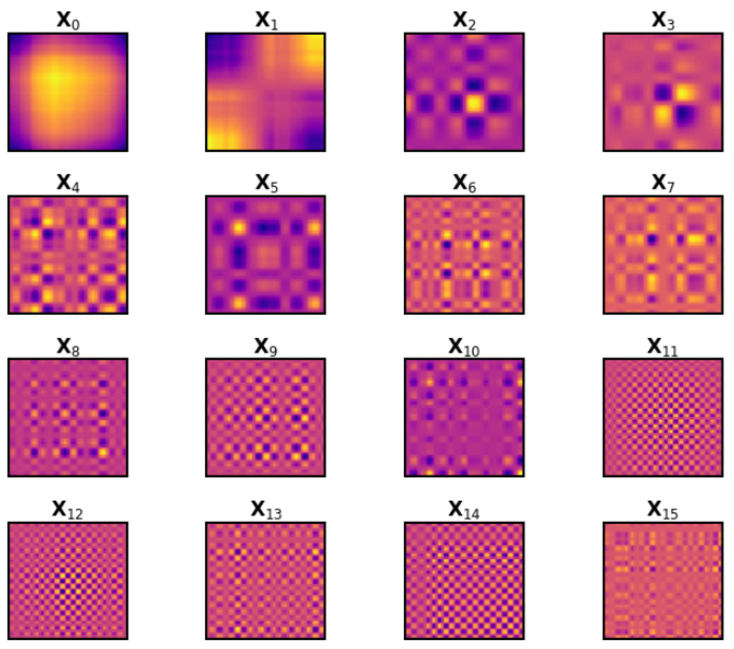
In an autoencoder, an image must be rolled into a single vector and a network must be built according to the constraints on the number of inputs. Therefore, the number of data sets used in this experiment averaged 160, which is about 2 min and 40 s of data. To match the number of inputs, the 36 most preceding arrays of 160 were expanded at the end of the array and applied in two dimensions.

The vibration signal, which served as an input value, is a one-dimensional signal of $1\times 196$, the size of the input data was set to $14\times 14$. The feature map was identified through the convolution kernel and maxpooling is used for down sampling. The sigmoid function was used as an activation function, and Adam was used as an optimization function. The detailed architecture of CAE can be found in

Table 1. Architecture of Convolutional Autoencoder.

Layer	Output Size	Parameter
Conv2D	14, 14, 128	1280
MaxPooling2D	7, 7, 128	0
Conv2D	7, 7, 128	147,584
UpSampling2D	14, 14, 128	0
Conv2D	14, 14, 128	147,584
Conv2D	14, 14, 1	1153

.

4. Experiment and Results

4.1. Data and Experiment Environment

In this experiment, data from CNC Machine, a production facility of Synswin Co., Ltd., located in Changwon, Korea, were used. The data used in the experiment is vibration data. The vibration data was collected from the MSENS-AC sensor via RS485 communication, and the data was collected by the IIoT installed in the field. The sampling rate of the applied sensor was 100 Hz and supported a 115,200 baudrate. Three-axis data was collected according to the characteristics of the gyro sensor. The data used in the double experiment was X-axis data. Data was collected on a 1000 ms basis, and examples of used data shown in Figure 7.

The data was collected during three days, from 5 October to 7 October 2021. The data matched to the manufactured product consists of an average of 552 data sets per day, with a total of 1700 data sets, and has 160 data per set. Therefore, experiment was conducted with 272,000 data. The data were all collected through sensors on the same CNC.

The computer used in this experiment included Intel Corei7-8700k, 3.7 Ghz, six-core twelve threads, 16 GB of CPU, and a GPU of Geforce RTX2080Ti. A Jetson nano from Nvidia was used as the EID used as a data collection, data reproduction, and as a classifier. Tensorflow 2.0 version and Python 3.7 were used in the software environment. The hardware and software specifications used for the experiments are listed in

Table 2. Hardware and software experimental environment setting.

Hardware Environment		Software Environment
PC	EID	PC	EID
CPU: Intel Core i7-8700K 3.7 Ghz six-core twelve threads 16 GB	CPU: 4 core ARM A57 1.43 GHz	Windows Tensorflow 2.0	Linux Tensorflow 2.0
GPU: Geforce RTX 2080Ti	GPU: 128 Core Maxwell 482 GFLOPs(FP16)	Python 3.7	Python 3.6

.

4.2. Evaluation Indicators and Experimental Methods

There are various evaluation scales in the data classification problem. In addition, various methods of performance evaluation according to the learning method have also been proposed. Circuit performance evaluation indicators were used according to the characteristics of the model used in this study. The mean absolute error (MAE) is a value averaged by converting the difference between the actual value and the predicted value into an absolute value, from which information on the loss of the model can be known. Root mean square error (RMSE) is the same as mean square error except for the root, but the root was used because it has a characteristic that is larger than the actual error mean when obtaining the square of the error. The formula used as an evaluation index is as follows.

$$RMSE=\sqrt{\frac{1}{N}\sum _N^{i=1}{(y_i-{\widehat{y}}_i)}^2}$$

(9)

$$MAE=\frac{1}{N}\sum _N^{i=1}\left|(y_i-{\widehat{y}}_i)\right|$$

(10)

This paper is largely divided into two parts. First, data regeneration was tested using Fourier transform and wavelet transform to evaluate the performance of SSA, which introduces data regeneration techniques. The following regenerated data was applied to unsupervised learning models such as autoencoder, autoencoder LSTM, and Convolutional Autoencoder to compare the performance of the model. Finally, the threshold value was obtained through the loss distribution chart for the best-performing model to prove the possibility of abnormality detection in the dataset.

4.3. Results

4.3.1. Data Regeneration Performance Comparison

Two methods were selected to verify the performance of the SSA technique used for data conversion. Short-time fourier transform (STFT) and wavelet transform. In STFT, a long signal that changes over time is divided into short time units and then Fourier transform is applied.

The Wavelet Transform increases time-time resolution and lowers frequency resolution for signals with high frequency components. For signals with low frequency components, frequency resolution is increased, and time resolution is decreased. Unlike Fourier transforms, which use sinusoidal curves with infinite time axes as fundamental functions, wavelet transforms use time-limited wavelet functions as fundamental functions.

Therefore, the experiment was conducted by applying STFT and wavelet transform to the same data set for data conversion and regeneration of the Singular Spectrum Analysis technique used in the proposed data classification. The experimental results are as follows.

Similarity was demonstrated in the order of reconstruction data, wavelet transform, Fourier transform and through the SSA technique as a result of reconstruction the value of the input data as illustrated in Figure 8a. As a result of visually examining the elementary matrix in Figure 9, it can be observed that the diagonal structure of the trajectory matrix is lacking. Without examining vectors related to the elementary matrix or reconstructing the time series of each component, the i-th elementary matrix figure implies the properties of each component, such as trend, periodicity, or noise. From the beginning, it can be observed that the L and K lagged vectors show relatively slow changes throughout the matrix, indicating a trend of data, and showing a distinct check pattern, indicating periodicity. Because the subsequent matrix becomes blurred again, the subsequent matrix is highly related to the noise of the time series.

According to the relative contribution graph in Figure 10a, the contribution changes at the time point when i = 1. In addition, in Figure 10b, the first ten component values based on the point contributed $98\%$ to the expansion of the basic matrix. Figure 10 is the result of accumulating $X_i$ components according to the contribution graph. The example output data by combining the X components can be seen in Figure 11.

4.3.2. Learning Results by Deep Learning Model

The following results were obtained according to the techniques introduced through previous studies and the order of experiments. Loss values and validation loss values were presented on the graph according to the performance index. First, the existing data were used and applied to each model.

The results of the experiment with the original data, demonstrated a stable loss reduction of less than 10 epochs, as shown in Figure 12. For each deep learning model, the final loss values were 0.095, 0.092, and 0.03 with the autoencoder, autoencoder short and long-term memory, and convolutional autoencoder.

The experiment conducted with the Fourier transformed data demonstrated as stable loss reduction at less than 10 epochs, as shown in Figure 13. For each deep learning model, the final loss values were 0.1155, 0.0661, and 0.0048 with the autoencoder, autoencoder LSTM, and CAE. It was observed that the autoencoder learning effect of the Fourier transformed data was not higher than that of the original data.

The experimental results with the wavelet data demonstrated a stable loss reduction at less than 10 epochs for each deep learning model in Figure 14, the final loss values were 0.0843, 0.0844, and 0.0347 for the autoencoder, autoencoder short and long-term memory, and convolutional autoencoder, respectively. It showed better performance than the original data and Fourier transformed data. As in Figure 15, the experimental results for the data regenerated with SSA demonstrated a stable loss reduction at less than 10 epochs. For each deep learning model, the final loss value was 0.0823, 0.0817, and 0.0178 with the autoencoder, autoencoder short and long-term memory, and convolutional autoencoder, respectively.

Table 3. The results of deep learning model learning according to each reconstruction data.

	Original			FFT Transform			Wavelet Transform			Singular Spectrum Analysis
	AE	AELSTM	CAE	AE	AELSTM	CAE	AE	AELSTM	CAE	AE	AELSTM	CAE
RMSE	0.303	0.294	0.17	0.35	0.23	0.07	0.291	0.290	0.173	0.283	0.27	0.122
MAE	0.095	0.092	0.03	0.116	0.066	0.0048	0.084	0.084	0.034	0.082	0.081	0.017

lists the model performances organized according to each data transform.

4.3.3. Data Classification

According to the results of the previous experiment, the performance of the SSA technique was evaluated by comparing it with other models, and the learning rate of the Convolutional Auto-encoder was high. Therefore, a distribution graph for the loss rate was drawn to use the SSA-CAE-based model in this proposed architecture. As confirmed in Figure 7, there is a time of 20 s at the start and end of machining. We conducted model learning in a cloud environment and imported the learned model into the EID, and the classification time was measured to be less than 15 s on average.

As shown in Figure 16, the loss distribution graph has normally distributed around a fifth of 0.1, and the output value is obtained according to the number of decimal places to obtain the threshold.

Abnormal detection was possible based on the threshold value of 0.02391 in

Table 4. Result of selecting threshold value according to loss value.

Loss_mae	Threshold
0.021355	0.02391
0.018467	0.02391
0.017650	0.02391
0.0198808	0.02391

. By inputting the model generated in the edge device, the classification of normal data on the test data of 6 November 2021 was achieved 100%, and the classification of abnormal data was achieved 99% in Figure 17.

5. Conclusions

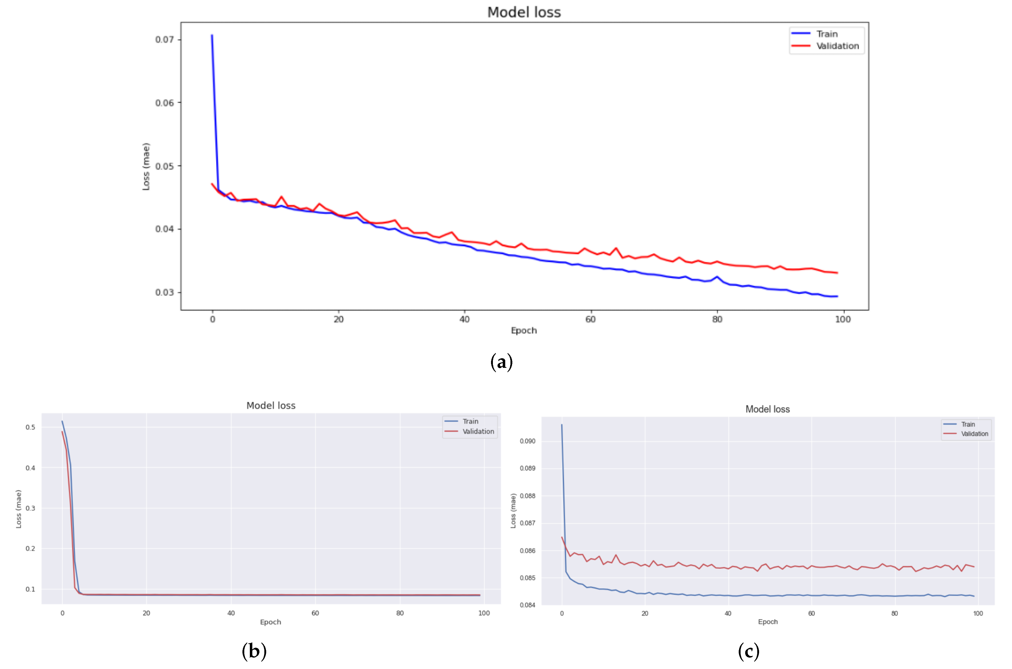
Data pre-processing is a very important task in data analysis. In particular, in machine learning and deep learning, pre-processing of data is a very common and important problem that must be addressed. To this end, techniques and libraries for automatic pre-processing have been studied and developed. The contribution of this paper is that, first, it proposes a big data storage method that can be used for smart factories. By systematizing data separation, “Product with Data” can be configured through product-level storage rather than previous storage methods. In addition, in the analysis, it is the basis for detailed research on data divided by units without pre-processing. Second, in previous studies, a labeling architecture for class imbalance occurring in the manufacturing industry was proposed by combining the data regeneration model and the deep learning model. This study puts a structural distinction between the edge and cloud in a way focused on computing rather than a model-oriented learning method, allowing model learning to be learned in the cloud and model performance to be performed in edge. In order to confirm whether these contributions have practical utility value, this study experimented with noise reduction and abnormal data set classification of data using data collected in the actual field, and verified the effect by proposing an effective classification architecture.

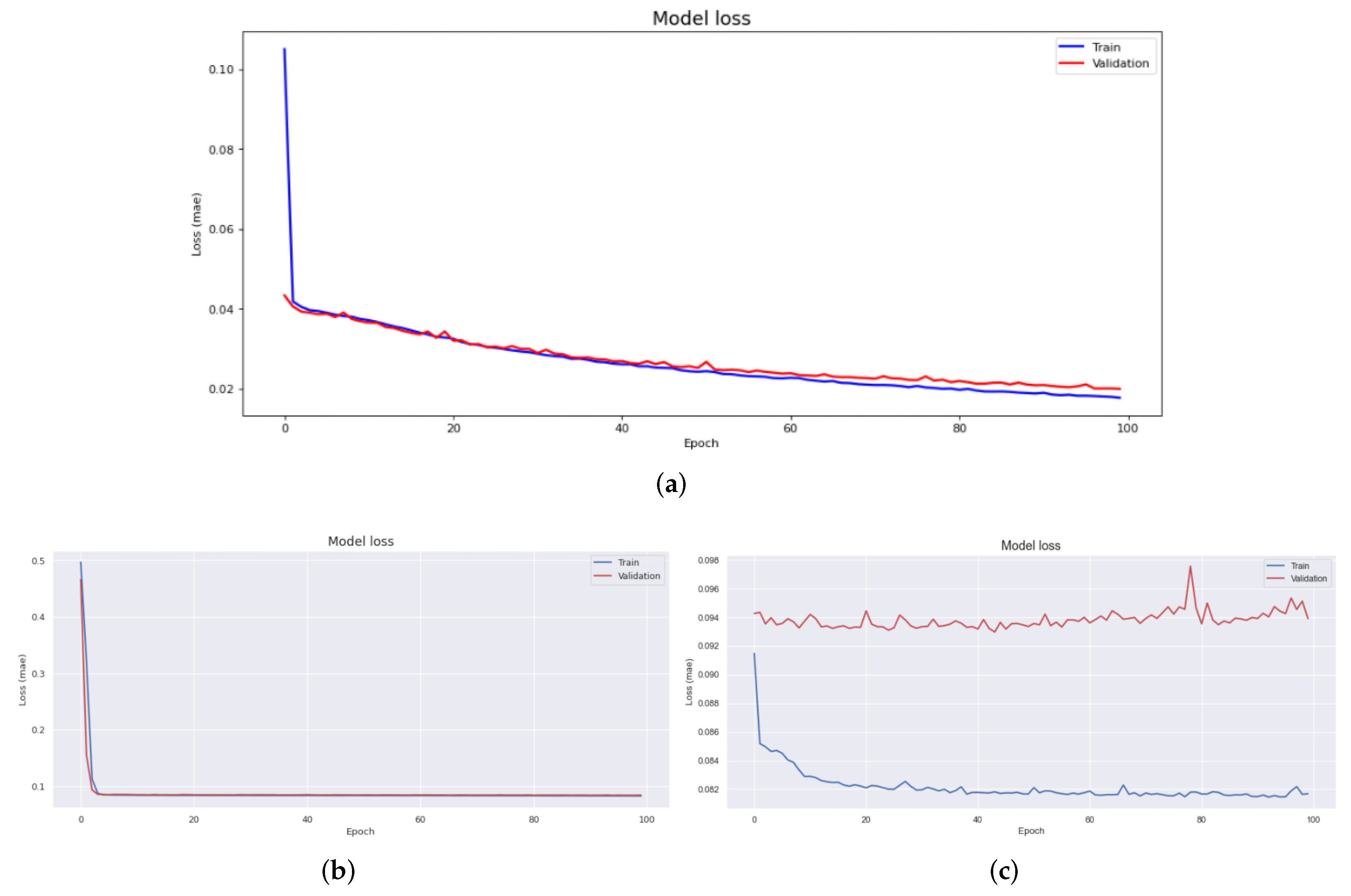
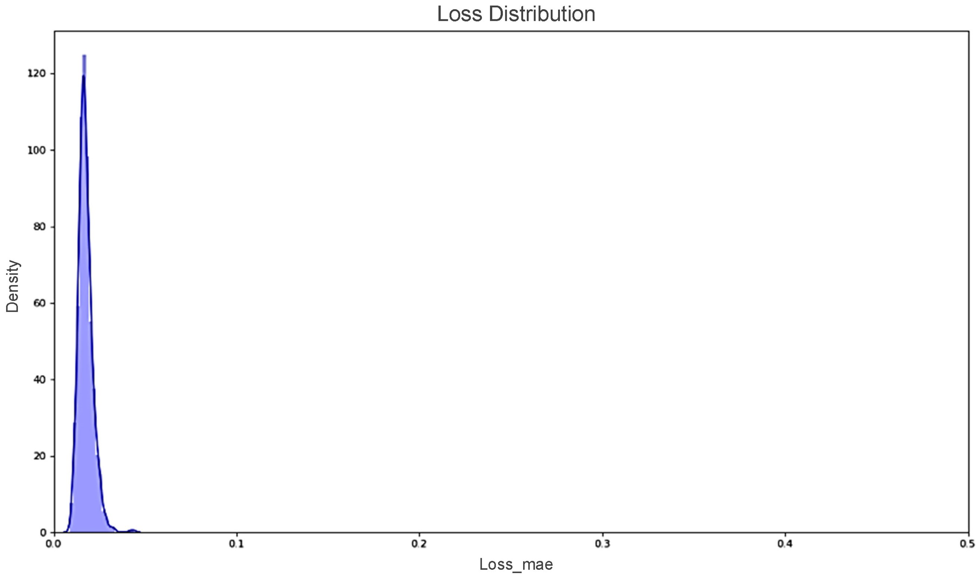
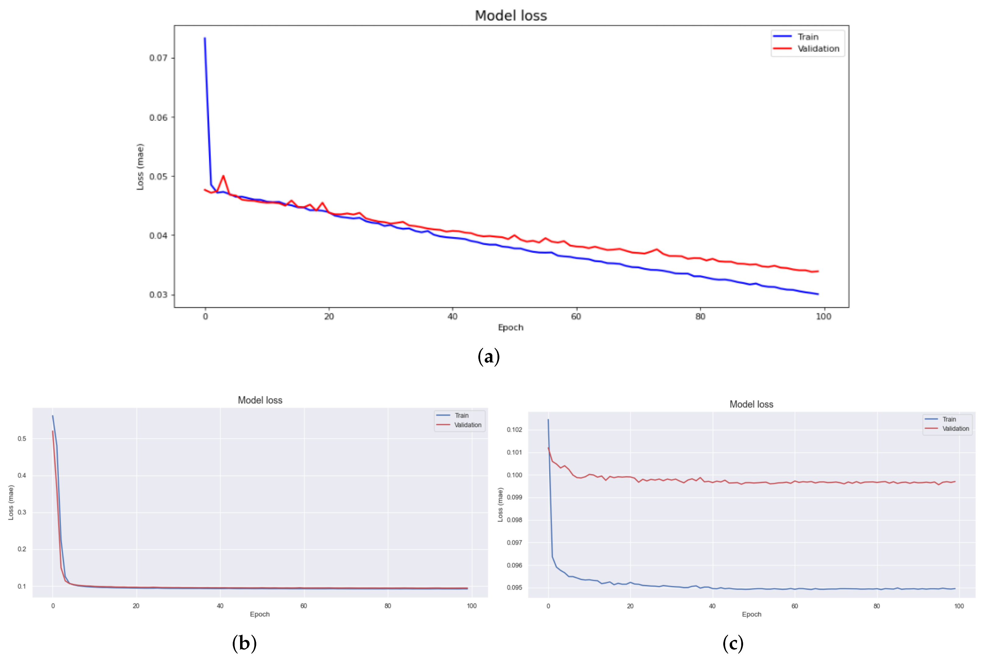
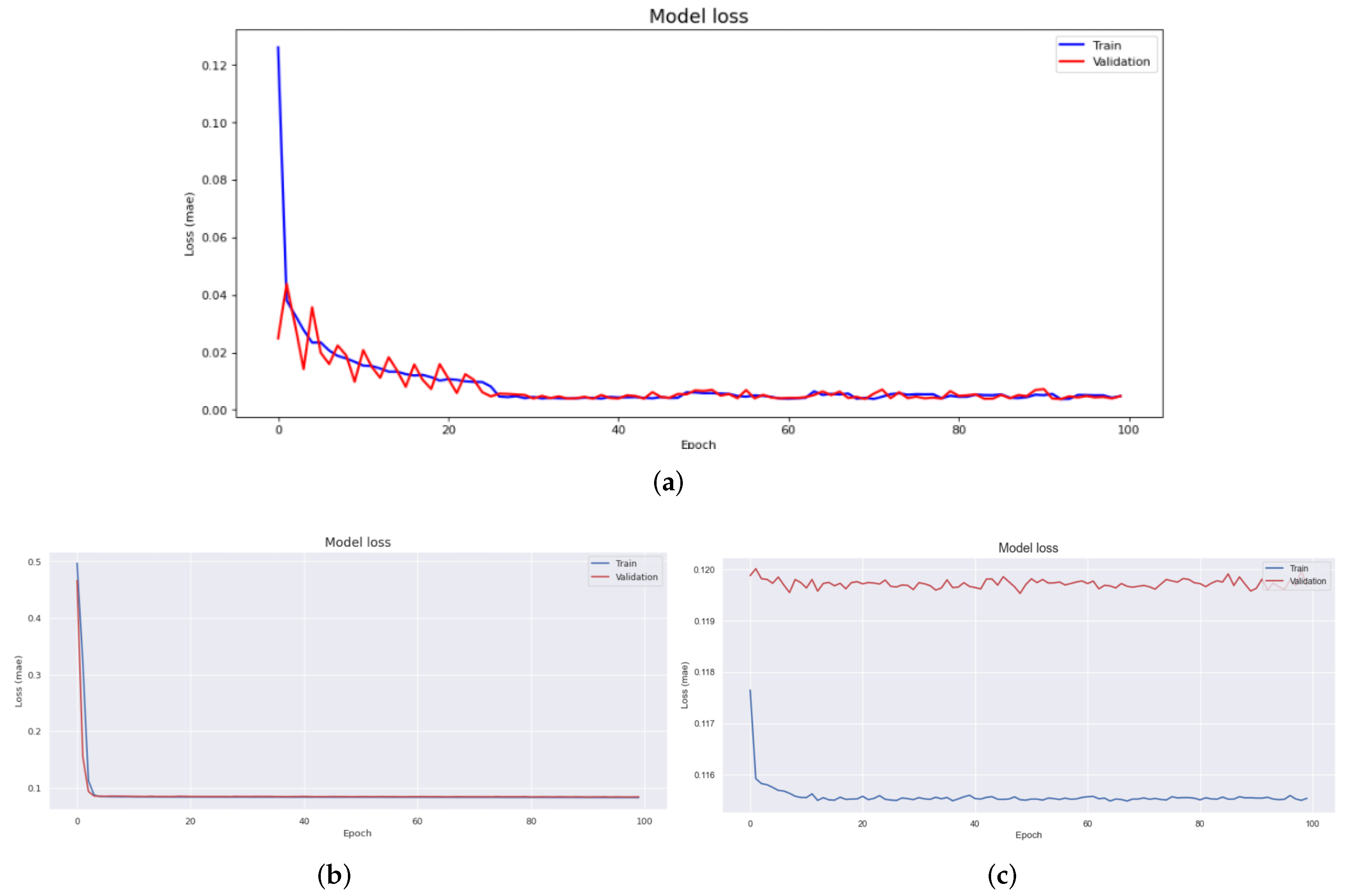
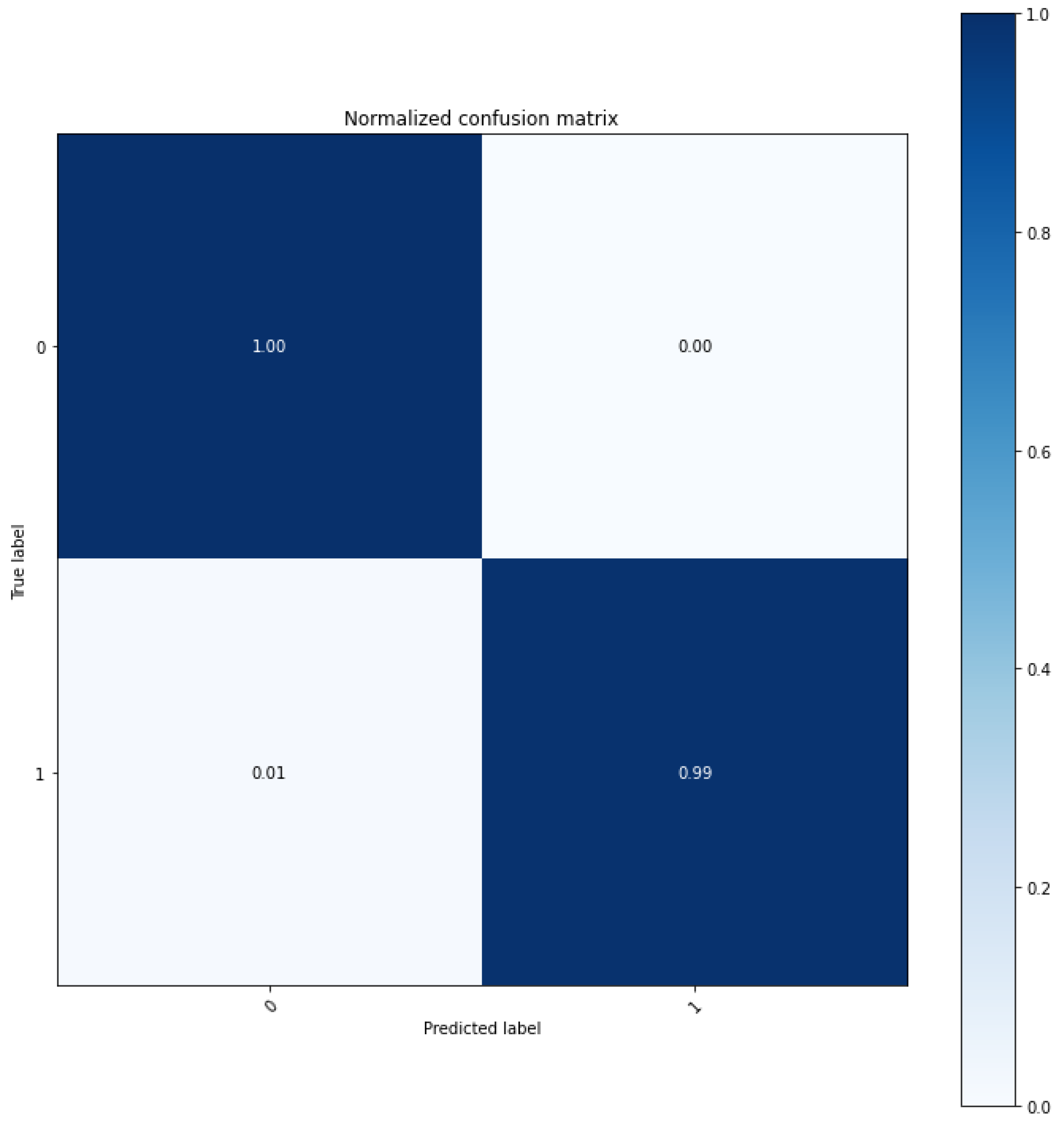
We demonstrated the excellence of the SSA technique for regenerative performance by using other transformation techniques, such as Fourier transform and wavelet transform techniques, as a control group to verify the performance of data collected at industrial sites. LSTM, a short- and long-term memory technique, was added, to the two controls, the autoencoder based convolutional autoencoder, and an unsupervised learning model. According to the experimental results, the experimental results applying CAE showed a difference more than 0.2 RMSE value compared to other results. In addition, MAE showed a difference almost 0.08. Therefore SSA-CAE showed a further improved modeling, and $99\%$ of classification was confirmed. It represents one error out of a total of 100 products.

Further research in the future may consider to apply according to the type of data collected in the field. To this end, the change and demonstration of the Edge Intelligence Device used in the experiment confirm the its applicability to other types of data. Further studies can also be conducted to determine whether $100\%$ classification rate results can be expected using additional studies on unsupervised learning other than the proposed SSA-CAE.