
A Machine Learning and Radiomics Approach in Lung Cancer for Predicting Histological Subtype

 ,
,  ,
,  ,
,  ,
,  and
and
Abstract
:1. Introduction
2. Materials
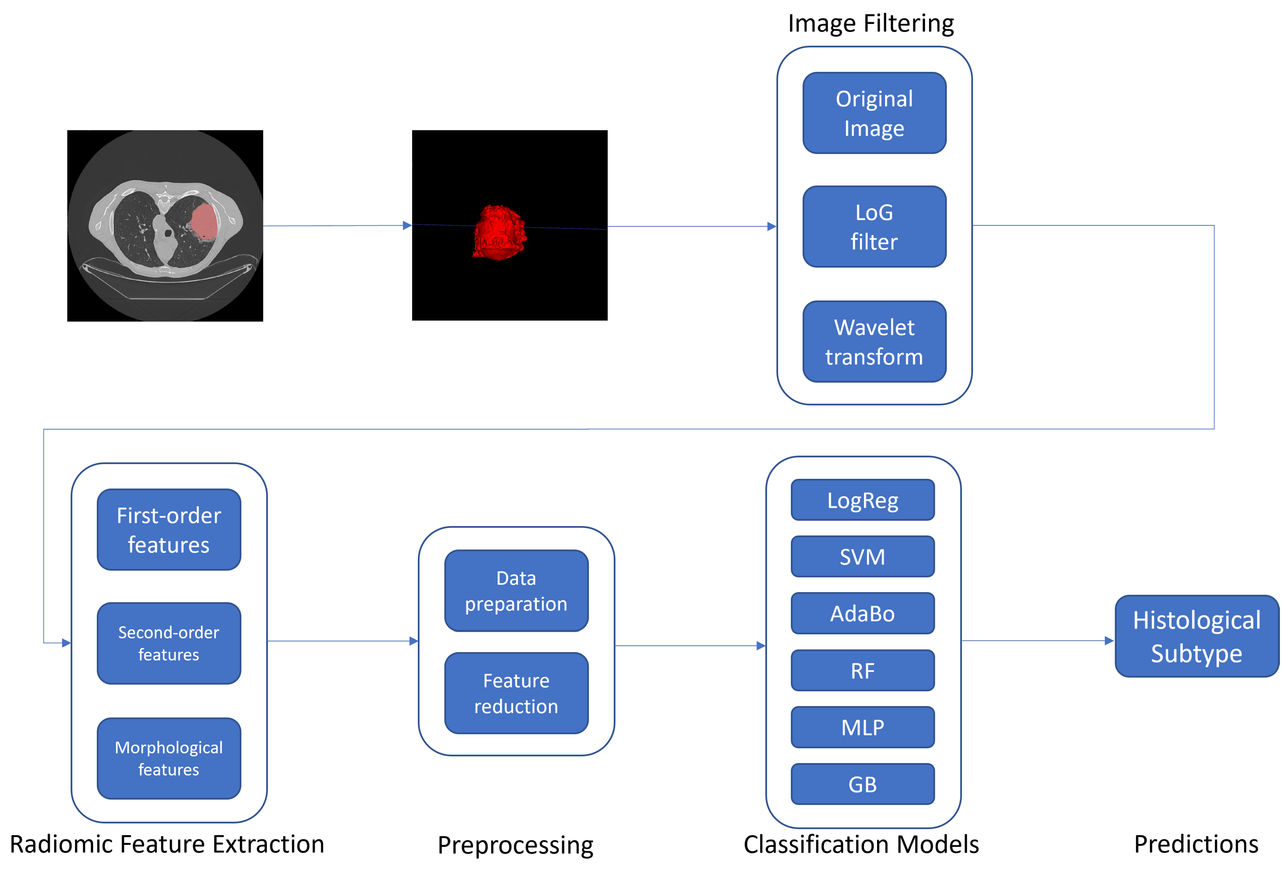
3. Methods
3.1. Radiomic Features
3.2. Feature Selection
Statistical Analysis
3.3. Classification
- Experiment 1: Internal cross-validation on each dataset (D1, D2, D3) separately; this experiment aimed to investigate if the radiomic signatures found by our approach could be discriminative for this classification task;
- Experiment 2: To train models on D1 and validate them on D2 and D3; this experiment aimed to investigate if the classifiers trained on a single dataset could perform on different datasets;
- Experiment 3: To train models on D1 and D2 (as a single dataset) and validate them on D3; this experiment aimed to investigate if increasing the training sample size could have improved the classification performance on the external validation;
- Experiment 4: Internal cross-validation merging D1, D2 and D3; this experiment aimed to investigate if considering all the datasets together could have led to a better performance than considering datasets separately, even at the cost of lower generalisation capabilities of the models.
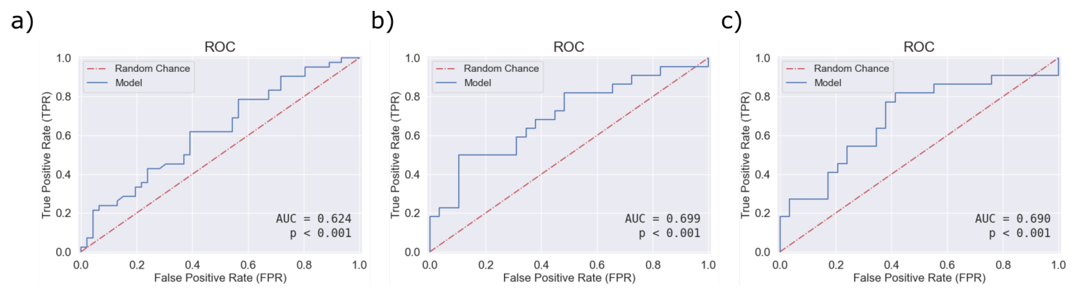
4. Results and Discussion
5. Conclusions
Author Contributions
Funding
Institutional Review Board Statement
Informed Consent Statement
Data Availability Statement
Conflicts of Interest
Abbreviations
| AdaBo | AdaBoost |
| LogReg | Logistic Regression |
| MLP | Multi Layer Perceptron |
| RF | Random Forest |
| SVM | Support Vector Machine |
| AUC | Area Under Curve |
| CT | Computed Tomography |
| C2 | Compacteness2 |
| CP | ClusterProminence |
| CS | ClusterShade |
| fMed | Firstorder Median |
| fS | Firstorder Skewness |
| GLNU | GrayLevelNonUniformity |
| LAHGLE | LargeAreaHighGrayLevelEmphasis |
| LRLGLE | LongRunLowGrayLevelEmphasis |
| SAE | SmallAreaEmphasis |
| SALGLE | SmallAreaLowGrayLevelEmphasis |
References
- Sung, H.; Ferlay, J.; Siegel, R.L.; Laversanne, M.; Soerjomataram, I.; Jemal, A.; Bray, F. Global Cancer Statistics 2020: GLOBOCAN Estimates of Incidence and Mortality Worldwide for 36 Cancers in 185 Countries. CA Cancer J. Clin. 2021, 71, 209–249. [Google Scholar] [CrossRef] [PubMed]
- Altini, N.; Cascarano, G.D.; Brunetti, A.; Marino, F.; Rocchetti, M.T.; Matino, S.; Venere, U.; Rossini, M.; Pesce, F.; Gesualdo, L.; et al. Semantic segmentation framework for glomeruli detection and classification in kidney histological sections. Electronics 2020, 9, 503. [Google Scholar] [CrossRef] [Green Version]
- Bevilacqua, V.; Brunetti, A.; Trotta, G.F.; Dimauro, G.; Elez, K.; Alberotanza, V.; Scardapane, A. A novel approach for Hepatocellular Carcinoma detection and classification based on triphasic CT Protocol. In Proceedings of the 2017 IEEE Congress on Evolutionary Computation (CEC), Donostia, Spain, 5–8 June 2017; pp. 1856–1863. [Google Scholar] [CrossRef]
- Robinson, P.N. Deep phenotyping for precision medicine. Hum. Mutat. 2012, 33, 777–780. [Google Scholar] [CrossRef]
- Tan, W.L.; Jain, A.; Takano, A.; Newell, E.W.; Iyer, N.G.; Lim, W.T.; Tan, E.H.; Zhai, W.; Hillmer, A.M.; Tam, W.L.; et al. Novel therapeutic targets on the horizon for lung cancer. Lancet. Oncol. 2016, 17, e347–e362. [Google Scholar] [CrossRef]
- Bevilacqua, V.; Brunetti, A.; Guerriero, A.; Trotta, G.F.; Telegrafo, M.; Moschetta, M. A performance comparison between shallow and deeper neural networks supervised classification of tomosynthesis breast lesions images. Cogn. Syst. Res. 2019, 53, 3–19. [Google Scholar] [CrossRef]
- Aerts, H.J. The potential of radiomic-based phenotyping in precision medicine: A review. JAMA Oncol. 2016, 2, 1636–1642. [Google Scholar] [CrossRef]
- Bevilacqua, V. Three-dimensional virtual colonoscopy for automatic polyps detection by artificial neural network approach: New tests on an enlarged cohort of polyps. Neurocomputing 2013, 116, 62–75. [Google Scholar] [CrossRef]
- European Society of Radiology (ESR) communications@myesr.org. Medical imaging in personalised medicine: A white paper of the research committee of the European Society of Radiology (ESR). Insights Into Imaging 2015, 6, 141–155. [Google Scholar] [CrossRef]
- Lee, G.; Lee, H.Y.; Park, H.; Schiebler, M.L.; van Beek, E.J.R.; Ohno, Y.; Seo, J.B.; Leung, A. Radiomics and its emerging role in lung cancer research, imaging biomarkers and clinical management: State of the art. Eur. J. Radiol. 2017, 86, 297–307. [Google Scholar] [CrossRef]
- Lambin, P.; Rios-Velazquez, E.; Leijenaar, R.; Carvalho, S.; Van Stiphout, R.G.P.M.; Granton, P.; Zegers, C.M.L.; Gillies, R.; Boellard, R.; Dekker, A.; et al. Radiomics: Extracting more information from medical images using advanced feature analysis. Eur. J. Cancer 2012, 48, 441–446. [Google Scholar] [CrossRef] [Green Version]
- Rahmim, A.; Schmidtlein, C.R.; Jackson, A.; Sheikhbahaei, S.; Marcus, C.; Ashrafinia, S.; Soltani, M.; Subramaniam, R.M. A novel metric for quantification of homogeneous and heterogeneous tumors in PET for enhanced clinical outcome prediction. Phys. Med. Biol. 2015, 61, 227. [Google Scholar] [CrossRef] [PubMed] [Green Version]
- Zwanenburg, A.; Vallières, M.; Abdalah, M.A.; Aerts, H.J.; Andrearczyk, V.; Apte, A.; Ashrafinia, S.; Bakas, S.; Beukinga, R.J.; Boellaard, R.; et al. The image biomarker standardization initiative: Standardized quantitative radiomics for high-throughput image-based phenotyping. Radiology 2020, 295, 328–338. [Google Scholar] [CrossRef] [PubMed] [Green Version]
- Kumar, V.; Gu, Y.; Basu, S.; Berglund, A.; Eschrich, S.A.; Schabath, M.B.; Forster, K.; Aerts, H.J.; Dekker, A.; Fenstermacher, D.; et al. Radiomics: The process and the challenges. Magn. Reson. Imaging 2012, 30, 1234–1248. [Google Scholar] [CrossRef] [PubMed] [Green Version]
- Rizzo, S.; Botta, F.; Raimondi, S.; Origgi, D.; Fanciullo, C.; Morganti, A.G.; Bellomi, M. Radiomics: The facts and the challenges of image analysis. Eur. Radiol. Exp. 2018, 2, 36. [Google Scholar] [CrossRef]
- Loconsole, C.; Cascarano, G.D.; Brunetti, A.; Trotta, G.F.; Losavio, G.; Bevilacqua, V.; Di Sciascio, E. A model-free technique based on computer vision and sEMG for classification in Parkinson’s disease by using computer-assisted handwriting analysis. Pattern Recognit. Lett. 2019, 121, 28–36. [Google Scholar] [CrossRef]
- Buongiorno, D.; Barsotti, M.; Barone, F.; Bevilacqua, V.; Frisoli, A. A linear approach to optimize an EMG-driven neuromusculoskeletal model for movement intention detection in myo-control: A case study on shoulder and elbow joints. Front. Neurorobot. 2018, 74. [Google Scholar] [CrossRef]
- Le, N.Q.K.; Kha, Q.H.; Nguyen, V.H.; Chen, Y.C.; Cheng, S.J.; Chen, C.Y. Machine learning-based radiomics signatures for EGFR and KRAS mutations prediction in non-small-cell lung cancer. Int. J. Mol. Sci. 2021, 22, 9254. [Google Scholar] [CrossRef]
- Aerts, H.J.W.L.; Velazquez, E.R.; Leijenaar, R.T.H.; Parmar, C.; Grossmann, P.; Carvalho, S.; Bussink, J.; Monshouwer, R.; Haibe-Kains, B.; Rietveld, D.; et al. Decoding tumour phenotype by noninvasive imaging using a quantitative radiomics approach. Nat. Commun. 2014, 5, 4006. [Google Scholar] [CrossRef]
- Bevilacqua, V.; Altini, N.; Prencipe, B.; Brunetti, A.; Villani, L.; Sacco, A.; Morelli, C.; Ciaccia, M.; Scardapane, A. Lung Segmentation and Characterization in COVID-19 Patients for Assessing Pulmonary Thromboembolism: An Approach Based on Deep Learning and Radiomics. Electronics 2021, 10, 2475. [Google Scholar] [CrossRef]
- Chaddad, A.; Kucharczyk, M.J.; Daniel, P.; Sabri, S.; Jean-claude, B.J.; Niazi, T.; Abdulkarim, B. Radiomics in Glioblastoma: Current Status and Challenges Facing Clinical Implementation. Front. Oncol. 2019, 9, 374. [Google Scholar] [CrossRef] [Green Version]
- Wakabayashi, T.; Ouhmich, F.; Gonzalez, C.; Emanuele, C.; Saviano, A.; Agnus, V.; Savadjiev, P.; Baumert, T.F.; Pessaux, P.; Marescaux, J.; et al. Radiomics in hepatocellular carcinoma: A quantitative review. Hepatol. Int. 2019, 13, 546–559. [Google Scholar] [CrossRef] [PubMed] [Green Version]
- Valdora, F.; Houssami, N.; Rossi, F.; Calabrese, M.; Stefano, A.; Pet, C.T. Rapid review: Radiomics and breast cancer. Breast Cancer Res. Treat. 2018, 169, 217–229. [Google Scholar] [CrossRef] [PubMed]
- Park, J.E.; Park, S.Y.; Kim, H.J.; Kim, H.S. Reproducibility and Generalizability in Radiomics Modeling: Possible Strategies in Radiologic and Statistical Perspectives. Korean J. Radiol. 2019, 20, 1124–1137. [Google Scholar] [CrossRef]
- Parmar, C.; Leijenaar, R.T.; Grossmann, P.; Velazquez, E.R.; Bussink, J.; Rietveld, D.; Rietbergen, M.M.; Haibe-Kains, B.; Lambin, P.; Aerts, H.J. Radiomic feature clusters and Prognostic Signatures specific for Lung and Head & neck cancer. Sci. Rep. 2015, 5, 11044. [Google Scholar] [CrossRef]
- Zhang, Y.; Oikonomou, A.; Wong, A.; Haider, M.A.; Khalvati, F. Radiomics-based Prognosis Analysis for Non-Small Cell Lung Cancer. Sci. Rep. 2017, 7, 46349. [Google Scholar] [CrossRef] [PubMed]
- Van Griethuysen, J.J.; Fedorov, A.; Parmar, C.; Hosny, A.; Aucoin, N.; Narayan, V.; Beets-Tan, R.G.; Fillion-Robin, J.C.; Pieper, S.; Aerts, H.J. Computational radiomics system to decode the radiographic phenotype. Cancer Res. 2017, 77, e104–e107. [Google Scholar] [CrossRef] [Green Version]
- Ferreira-Junior, J.R.; Koenigkam-Santos, M.; Magalhães Tenório, A.P.; Faleiros, M.C.; Garcia Cipriano, F.E.; Fabro, A.T.; Näppi, J.; Yoshida, H.; de Azevedo-Marques, P.M. CT-based radiomics for prediction of histologic subtype and metastatic disease in primary malignant lung neoplasms. Int. J. Comput. Assist. Radiol. Surg. 2020, 15, 163–172. [Google Scholar] [CrossRef]
- Linning, E.; Lu, L.; Li, L.; Yang, H.; Schwartz, L.H.; Zhao, B. Radiomics for Classifying Histological Subtypes of Lung Cancer Based on Multiphasic Contrast-Enhanced Computed Tomography. J. Comput. Assist. Tomogr. 2019, 43, 300–306. [Google Scholar] [CrossRef]
- Zhai, T.T.; Wesseling, F.; Langendijk, J.A.; Shi, Z.; Kalendralis, P.; van Dijk, V.L.; Hoebers, F.; Steenbakkers, R.J.H.M.; Dekker, A.; Wee, L.; et al. External validation of nodal failure prediction models including radiomics in head and neck cancer. Oral Oncol. 2021, 112, 105083. [Google Scholar] [CrossRef]
- Wu, W.; Parmar, C.; Grossmann, P.; Quackenbush, J.; Lambin, P.; Bussink, J.; Mak, R.; Aerts, H.J. Exploratory study to identify radiomics classifiers for lung cancer histology. Front. Oncol. 2016, 6, 71. [Google Scholar] [CrossRef] [Green Version]
- Grossmann, P.; Stringfield, O.; El-Hachem, N.; Bui, M.M.; Velazquez, E.R.; Parmar, C.; Leijenaar, R.T.; Haibe-Kains, B.; Lambin, P.; Gillies, R.J.; et al. Defining the biological basis of radiomic phenotypes in lung cancer. eLife 2017, 6, e23421. [Google Scholar] [CrossRef] [PubMed]
- Yushkevich, P.A.; Piven, J.; Cody Hazlett, H.; Gimpel Smith, R.; Ho, S.; Gee, J.C.; Gerig, G. User-Guided {3D} Active Contour Segmentation of Anatomical Structures: Significantly Improved Efficiency and Reliability. Neuroimage 2006, 31, 1116–1128. [Google Scholar] [CrossRef] [PubMed] [Green Version]
- Gillies, R.J.; Kinahan, P.E.; Hricak, H. Radiomics: Images are more than pictures, they are data. Radiology 2016, 278, 563–577. [Google Scholar] [CrossRef] [PubMed] [Green Version]
- Haralick, R.M.; Dinstein, I.; Shanmugam, K. Textural Features for Image Classification. IEEE Trans. Syst. Man Cybern. 1973, SMC-3, 610–621. [Google Scholar] [CrossRef] [Green Version]
- Galloway, M.M. Texture analysis using gray level run lengths. Comput. Graph. Image Process. 1975, 4, 172–179. [Google Scholar] [CrossRef]
- Chu, A.; Sehgal, C.M.; Greenleaf, J.F. Use of gray value distribution of run lengths for texture analysis. Pattern Recognit. Lett. 1990, 11, 415–419. [Google Scholar] [CrossRef]
- Thibault, G.; Fertil, B.; Navarro, C.; Pereira, S.; Cau, P.; Levy, N.; Sequeira, J.; Mari, J.l. Texture Indexes and Gray Level Size Zone Matrix Application to Cell Nuclei Classification. In Proceedings of the 2009 10th International Conference on Document Analysis and Recognition, Barcelona, Spain, 26–29 July 2009; pp. 140–145. [Google Scholar]
- Sun, C.; Wee, W.G. Neighboring gray level dependence matrix for texture classification. Comput. Vision Graph. Image Process. 1983, 23, 341–352. [Google Scholar] [CrossRef]
- Amadasun, M.; King, R. Texural Features Corresponding to Texural Properties. IEEE Trans. Syst. Man Cybern. 1989, 19, 1264–1274. [Google Scholar] [CrossRef]
- Wang, P.; Pei, X.; Yin, X.P.; Ren, J.L.; Wang, Y.; Ma, L.Y.; Du, X.G.; Gao, B.L. Radiomics models based on enhanced computed tomography to distinguish clear cell from non-clear cell renal cell carcinomas. Sci. Rep. 2021, 11, 13729. [Google Scholar] [CrossRef]
- Altini, N.; Brunetti, A.; Mazzoleni, S.; Moncelli, F.; Zagaria, I.; Prencipe, B.; Lorusso, E.; Buonamico, E.; Carpagnano, G.E.; Bavaro, D.F.; et al. Predictive Machine Learning Models and Survival Analysis for COVID-19 Prognosis Based on Hematochemical Parameters. Sensors 2021, 21, 8503. [Google Scholar] [CrossRef]


| Dataset | Acronym | Sample | Image Modality | Type of Data |
|---|---|---|---|---|
| Dataset1 [32] | D1 | 262 | CT scans (89% contrast-enhanced) | Radiomic features, clinical data, genomic features |
| Dataset2 [32] | D2 | 89 | CT scans (71% contrast-enhanced) | Radiomic features, clinical data, genomic features |
| Dataset3 | D3 | 51 | Unenhanced CT scans | Radiomic features, hystological type |
| Feature Name | Mean | Std | Median | IQR | p-Value | ||||
|---|---|---|---|---|---|---|---|---|---|
| LUAD | Other | LUAD | Other | LUAD | Other | LUAD | Other | BH | |
| O_glcm_Autocorrelation | −0.2449 | 0.3470 | 0.8658 | 1.0672 | −0.3783 | 0.3439 | 1.2597 | 1.6090 | 0.0011 * |
| O_glcm_CP | −0.1698 | 0.2334 | 0.6434 | 1.3142 | −0.3974 | −0.1727 | 0.6376 | 1.0980 | 0.1406 |
| O_glszm_SALGLE | 0.1244 | −0.1560 | 1.0337 | 0.9384 | −0.0800 | −0.2190 | 0.9632 | 1.2388 | 0.1993 |
| O_firstorder_Mean | −0.1230 | 0.1965 | 1.1544 | 0.6577 | 0.1154 | 0.2908 | 0.8318 | 0.6643 | 0.0207 * |
| W-HHH_glcm_JointEnergy | −0.0526 | 0.0776 | 1.0925 | 0.8696 | −0.3825 | −0.1291 | 0.8819 | 1.0823 | 0.1591 |
| W-HHH_glcm_Imc1 | −0.0565 | 0.0869 | 1.0679 | 0.9050 | 0.1817 | 0.3549 | 0.7541 | 0.6453 | 0.1993 |
| W-HHH_firstorder_Energy | −0.0917 | 0.1253 | 0.1835 | 1.5198 | −0.1577 | −0.1340 | 0.0651 | 0.1342 | 0.1591 |
| W-LHH_firstorder_Energy | −0.1404 | 0.1940 | 0.5804 | 1.3641 | −0.3493 | −0.2788 | 0.2868 | 0.6737 | 0.1406 |
| W-LHH_firstorder_Median | 0.1818 | −0.2496 | 1.1321 | 0.7358 | −0.0498 | −0.1823 | 0.6231 | 0.4321 | 0.0036 * |
| W-LLH_glcm_Correlation | −0.0680 | 0.0908 | 1.0421 | 0.9493 | 0.0318 | 0.1667 | 1.1192 | 0.9215 | 0.1993 |
| Model | Hyperparameters | Value |
|---|---|---|
| LogReg | max_iter | 100 |
| penalty | 12 | |
| C | 1.0 | |
| SVM | kernel | rbf |
| C | 1.0 | |
| penalty | 12 | |
| AdaBo | n_estimators | 50 |
| learning_rate | 1.0 | |
| RF | n_estimators | 100 |
| criterion | gini | |
| max_depth | None | |
| MLP | neurons_per_layer | 100 |
| hidden_layers | 1 | |
| b1 | 0.9 | |
| b2 | 0.999 | |
| solver | adam | |
| learning_rate_init | 0.001 | |
| max_iter | 200 | |
| early_stop | None | |
| penalty | 12 | |
| alpha | 0.0001 | |
| activation | relu | |
| GB | learning_rate | 0.1 |
| n_estimators | 100 | |
| criterion | friedman_mse |
Publisher’s Note: MDPI stays neutral with regard to jurisdictional claims in published maps and institutional affiliations. |
© 2022 by the authors. Licensee MDPI, Basel, Switzerland. This article is an open access article distributed under the terms and conditions of the Creative Commons Attribution (CC BY) license (https://creativecommons.org/licenses/by/4.0/).
Share and Cite
Brunetti, A.; Altini, N.; Buongiorno, D.; Garolla, E.; Corallo, F.; Gravina, M.; Bevilacqua, V.; Prencipe, B. A Machine Learning and Radiomics Approach in Lung Cancer for Predicting Histological Subtype. Appl. Sci. 2022, 12, 5829. https://doi.org/10.3390/app12125829
Brunetti A, Altini N, Buongiorno D, Garolla E, Corallo F, Gravina M, Bevilacqua V, Prencipe B. A Machine Learning and Radiomics Approach in Lung Cancer for Predicting Histological Subtype. Applied Sciences. 2022; 12(12):5829. https://doi.org/10.3390/app12125829
Chicago/Turabian StyleBrunetti, Antonio, Nicola Altini, Domenico Buongiorno, Emilio Garolla, Fabio Corallo, Matteo Gravina, Vitoantonio Bevilacqua, and Berardino Prencipe. 2022. "A Machine Learning and Radiomics Approach in Lung Cancer for Predicting Histological Subtype" Applied Sciences 12, no. 12: 5829. https://doi.org/10.3390/app12125829
APA StyleBrunetti, A., Altini, N., Buongiorno, D., Garolla, E., Corallo, F., Gravina, M., Bevilacqua, V., & Prencipe, B. (2022). A Machine Learning and Radiomics Approach in Lung Cancer for Predicting Histological Subtype. Applied Sciences, 12(12), 5829. https://doi.org/10.3390/app12125829