Improving on Atmospheric Turbulence Profiles Derived from Dual Beacon Hartmann Turbulence Sensor Measurements

Featured Application

Generation of optical turbulence profiles.

Abstract

Atmospheric turbulence is an inevitable source of wavefront distortion in all fields of long range laser propagation and sensing. However, the distorting effects of turbulence can be corrected using wavefront sensors contained in adaptive optics systems. Such systems also provide deeper insight into surface layer turbulence, which is not well understood. A unique method of profile generation by a dual source Hartmann Turbulence Sensor (HTS) technique is introduced here. Measurements of optical turbulence along a horizontal path were taken to create $C_n^2$ profiles. Two helium-neon laser beams were directed over an inhomogeneous horizontal path and captured by the HTS. The measured differential tilt variances imposed on the laser wavefronts were used in conjunction with a set of computed weighting functions to profile the turbulence over the sensing path. The weighting function matrix is inherently ill-conditioned, therefore, Tikhonov regularization was applied to produce accurate $C_n^2$ profiles. A distribution of sonic anemometers and a co-located boundary layer scintillometer (BLS) collected independent $C_n^2$ measurements to add confidence to the HTS profiles. The $C_n^2$ profiles generated by this approach agree very well with the auxiliary anemometer and scintillometer measurements. This method of producing turbulence profiles may be useful in future multi-conjugate adaptive optics applications.

1. Introduction

Turbulence is an unavoidable phenomenon that must be considered in any field relying on long range light propagation through the atmosphere, whether it be directed energy, satellite imagery, or surveillance from aircraft. Without corrections, the loss of beam quality or imaging resolution can be significant. Adaptive optics (AO) systems have become a standard solution to this issue. These systems measure the phase distortions of an incoming wavefront and use a deformable mirror to apply the conjugate phase to either an incoming or outgoing beam, thereby correcting the distortion. Typical AO systems use a singular measurement of the tips and tilts to correct the wavefront, but under conditions where turbulence is distributed unevenly along the sensing path, knowledge of the turbulence profile and several deformable mirrors in series (known as multi-conjugate AO) allows for more accurate corrections. The methodology presented here introduces a novel technique for computing reliable turbulence profiles and demonstrates that accurate profiles can be computed over an inhomogeneous path using a Hartmann Turbulence Sensor and optimized with Tikhonov regularization.

Scintillation detection and ranging, also knows as SCIDAR [1,2], uses a telescope to measure intensity fluctuations from a binary star pair to produce vertical $C_n^2$ profiles of the atmosphere [3]. Although effective, scintillation-based techniques are prone to saturation issues over long distances that are less detrimental to phase-based techniques. Slope detection and ranging, or SLODAR, is a phase-based remote sensing method used to generate vertical $C_n^2$ profiles by measuring wavefront Zernike tilts [4]. SLODAR is particularly useful in astronomy to generate turbulence profiles by observing the tilts from a binary star system. Previous work [5] describes a technique similar to SLODAR, but with a distinct methodology, that uses an HTS and two laser sources to profile turbulence over a path. By observing a binary star pair, SLODAR uses the auto-correlation and cross-correlations of incoming wavefront tilts to recover the normalized turbulence profile [4]. Then, by a technique called differential image motion monitoring (DIMM), the full integrated turbulence strength and $r_0$ estimates can be recovered [6]. The technique introduced in Section 2 also uses local wavefront tilts to recover the turbulence profile, but by entirely different methodology. Another similar phase-based technique to turbulence profiling centers around a process called difference in differential tilt variance, first described by Whiteley et al. [7].

This work used tilt measurements to generate $C_n^2$ profiles under varying conditions including time of day, cloud coverage, wind velocity, and an inhomogeneous sensing path (sections of grass and concrete). This method leverages differential angle of arrival measurements between two sources to reduce the common mode noise in the wavefront tilts caused by platform vibrations or angular tracking error. Similar dual-beacon techniques for turbulence profile generation have been introduced by Hickson et al. [8] and Sauvage et al. [9]. A Moore–Penrose pseudo-inversion method is used to generate the profiles from the weighting function and differential tilt variance matrices. This method minimizes the residual, but is sensitive to noise present in the data. The differential tilt variances are calculated by tracking the centroid motion of laser subimages on a subaperture array in a technique similar to the method described by Kovadlo et al. [10]. The weighting function matrix used to calculate the profile is ill-conditioned, and thus, Tikhonov regularization has been used to minimize the residual and the solution vectors. This method ultimately produces a noise-reduced profile. The $C_n^2$ profiles generated using the HTS measurements were validated through comparison with a co-located boundary layer scintillometer. Further confidence in the estimated HTS $C_n^2$ profiles was provided by comparison with four sonic anemometers distributed along the sensing path.

2. Materials and Methods

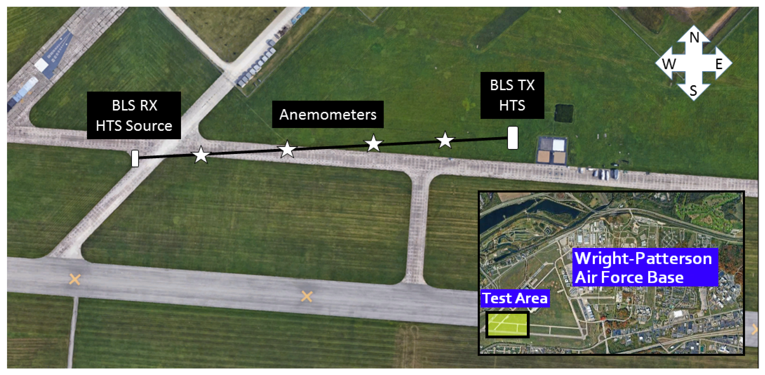
The sensing path chosen for this work is shown in Figure 1. The 511 m path was chosen for its inhomogeneity, with the first half grass and the second half concrete. The data presented in this study was captured on 25 July 2019 from 17:44 to 21:33 EST (UTC-4). The air temperature during testing was 28 °C on with wind speeds less than 5 mph and intermittent cloud coverage, which was captured by a net radiometer. Each set of tilt variance data contains 100 background frames with the laser beacons shut off and 1000 data frames with both lasers active.

The Hartmann Turbulence Sensor (HTS) is a Shack–Hartmann wavefront sensor based on a 16" Meade LX200 telescope. It was designed to provide time-efficient and accurate estimates of statistical parameters such as the Fried coherence length, $r_0$, the refractive index structure parameter, $C_n^2$, and the Greenwood frequency, $f_G$, all of which are key characteristics of optical turbulence [11]. The HTS was mounted on a floating suspension system within a trailer to protect the system from vibrations and weather during operation and transportation. A custom optics bench mounted in the sensor’s backplane contains a 32 × 32 lenslet array, relay optics, and a Vision Research Phantom v7.3 high speed camera capable of capturing up to 8639 frames/s [12].

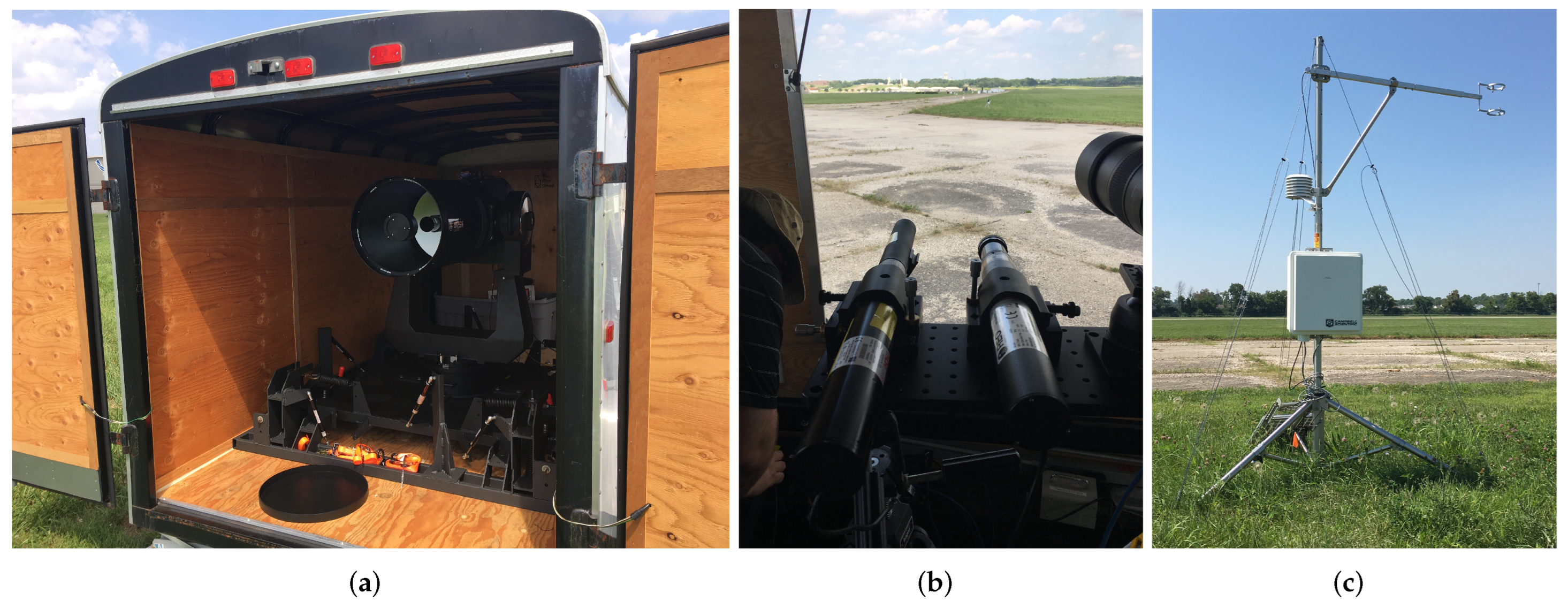
Four SATI/3A non-orthogonal sonic anemometers were mounted 2.64 m above the ground and distributed evenly along the path at points 100 m, 200 m, 300 m, and 400 m from the HTS. The HTS, laser beacon, and sonic anemometer setups are shown in Figure 2. The anemometers calculate point-like estimates of $C_n^2$ over a much smaller volume in space than the HTS technique. The anemometers capture measurements at 10 Hz, which are averaged into 1 min increments for the profile comparisons. The anemometers’ accuracy in sonic temperature measurements is $\pm 0.1$ ${}^{\circ }$C, which suggests measurement error is low relative to the $C_n^2$ estimates. Two of the anemometers measured over grass while the other two measured over concrete to help illustrate the expected local rise in turbulence over the concrete. Past experiments [13] have found a potential relation between the turbulence anisotropy and the wind direction with respect to the sensing path. Since the experimental path was roughly aligned with the prevailing winds, this effect was expected to be minimal. The HTS sensing path was horizontal and 1.5 m above ground level. The sonic anemometers were mounted over a meter higher than the HTS sensing path, and thus, saw weaker turbulence. This height difference was roughly corrected using an $h^{-4/3}$ conversion factor, where h is the height from ground [14]. This height correction is an approximation for turbulence variations with respect to altitude during typical daytime conditions ($C_n^2$ between ${10}^{-14}$ and ${10}^{-13} {\mathrm{m}}^{-2/3}$) when convective forces dominate the surface layer. The prevailing wind during this experiment was from the west and roughly parallel to the sensing path. Therefore, the turbulence that reached the HTS developed for about 250 m above the concrete and then for about 250 m above the grass. This not only emphasized the differences in turbulence strength over both parts, but also made the height correction more applicable over the full path.

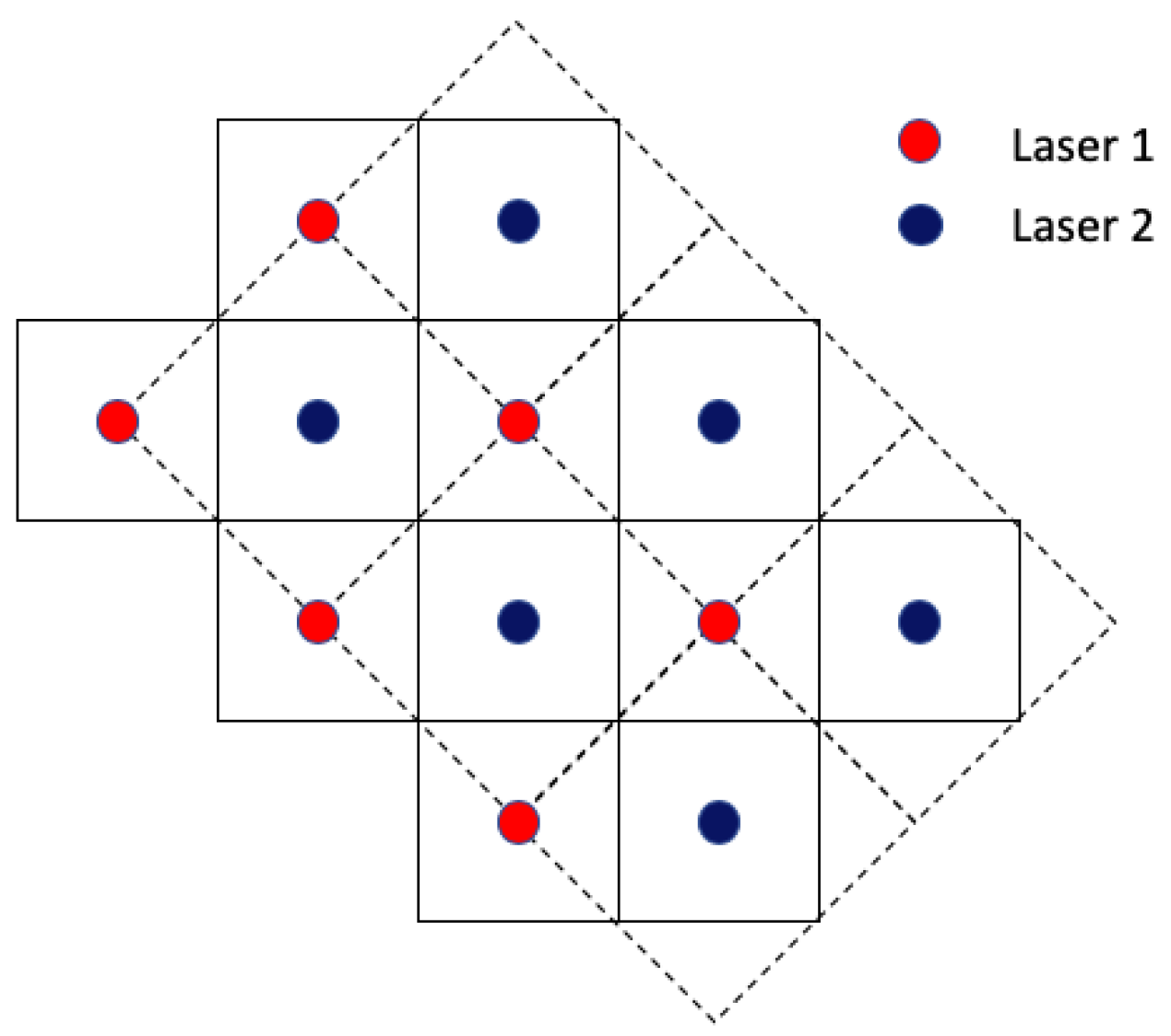
Two 2 mW 632.8 nm helium-neon laser beacons were mounted with an 11 cm separation at the opposite end of the sensing path from the HTS. The 11 cm separation ensured the laser subimages were roughly centered in the subaperture regions. Each laser was fitted with a beam diverger (with 0.5 inch apertures) for complete illumination of the HTS telescope. The beams are treated as spherical waves after exiting the divergers. The Phantom camera’s CCD is typically divided into 18 × 18 pixel subaperture regions when using a single beacon. To maximize the separation between both lasers’ respective subimages, the lenslet array was rotated by 45 degrees, which in turn changed the size of the subaperture regions from 18 × 18 pixels to 12.7 × 12.7 pixels as shown in Figure 3. For simplicity, the telescope magnification was slightly adjusted such that the subimages lie within 13 × 13 pixel boxes. The 11 cm laser separation ensured the subimages formed by the lenslet array were centered within these respective regions. During periods of strong turbulence, the subimages can spill outside of their allocated regions affecting data processing and profile computation. Each lenslet has a 146 $\mathsf{\mu }$m diameter and a 5.2 mm focal length. The lenslet array has a 150 $\mathsf{\mu }$m pitch [12]. The spaces between are masked with chrome to block light not passing through the lenslets [15].

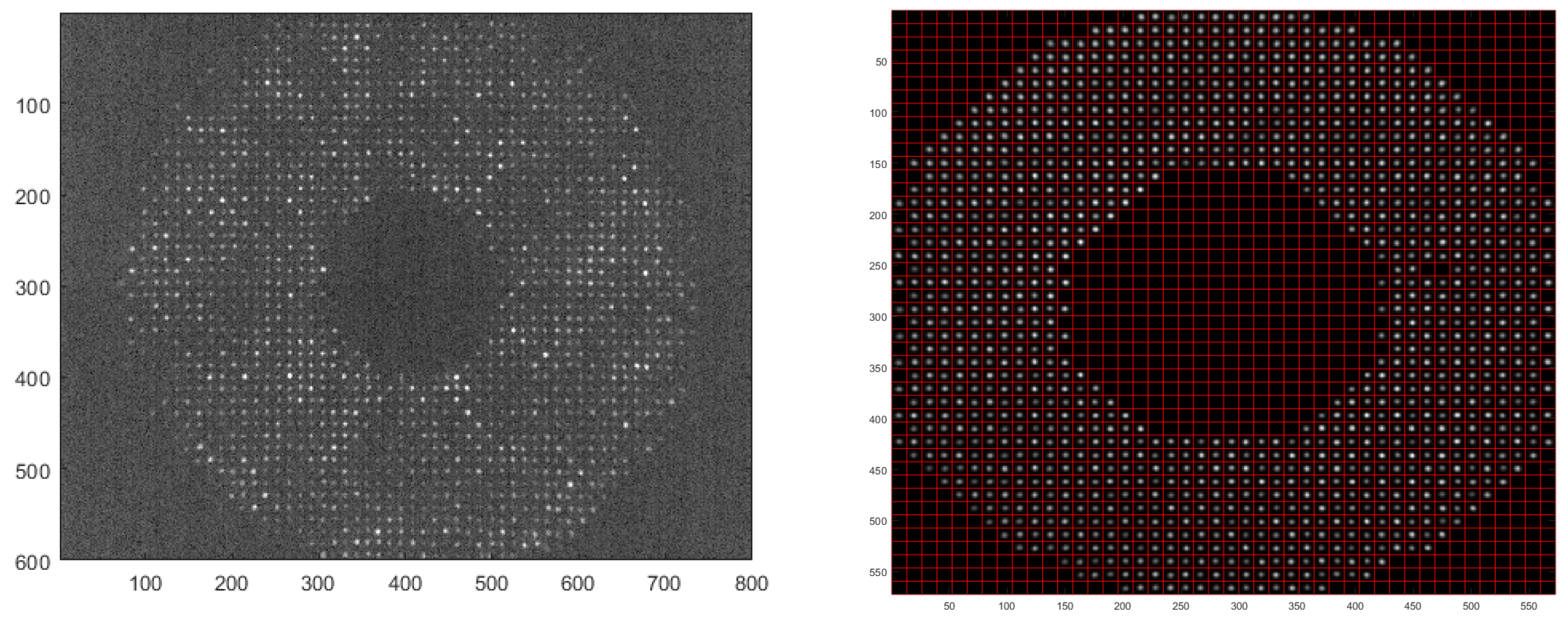
The Phantom camera captures the subimage motion in 600 × 800 pixel frames, which are cropped to 572 × 572 pixels for processing. A mask is then applied to the data frames to cover subapertures that are not fully illuminated due to proximity to the telescope aperture and the central obscuration. Flawed or blurred subapertures are also covered by the mask. This has a negligible effect on the solution due to the large sample size of additional subapertures available for the statistical calculations. Once the mask is applied, an auto-focusing algorithm is used to calculate the centroid of the mean frame of each subimage and then correct the tracking windows to center on the same respective points. This collection of data is used to calculate the differential tilt variances for all crossing and non-crossing sensing paths. A comparison of an initial HTS data frame against a cropped, background subtracted, masked, and auto-focused frame is shown in Figure 4.

2.1. Weighting Functions

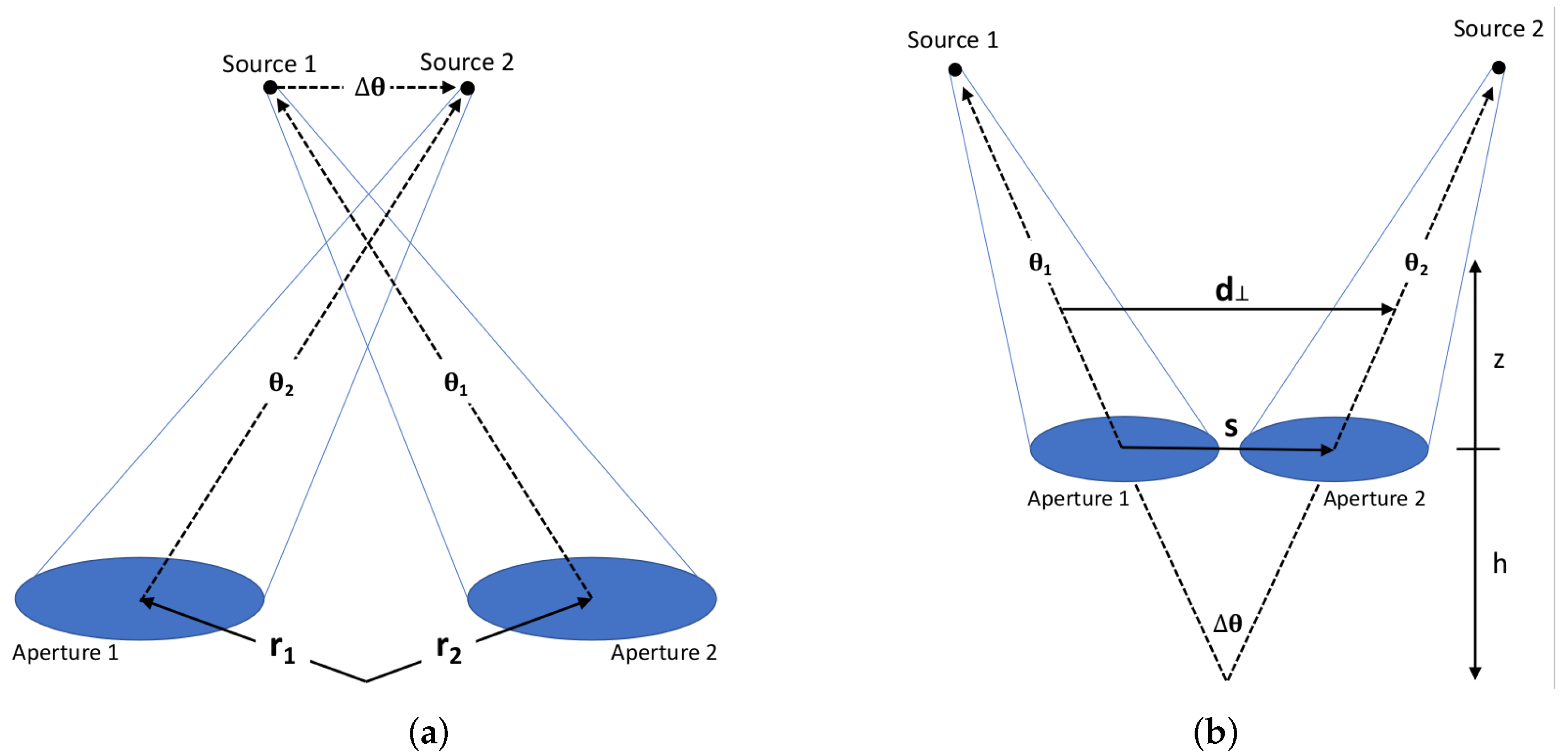
The weighting functions used in this work have been derived in previous papers [16,17]. They were derived through geometric optics approximations and therefore neglect some effects of diffraction. The weighting functions for two sensing paths that cross between the laser beacons and two subapertures as shown in Figure 5a are given by

$$\begin{array}{cc}\hfill f_{dc}\left(z\right)& =-2.91{\left(\frac{16}{\pi }\right)}^2{D}^{-1/3}{\int }_0^{2\pi }d\theta {\int }_0^{1}du\hfill \\ & \left[\left(uco{s}^{-1}u\right)-u^2(3-2u^2)\sqrt{1-u^2}\right]·\{{\left|u\left(1-\frac{z}{L}\right)\right|}^{5/3}\hfill \\ & -\frac{1}{2}{\left[u^2{\left(1-\frac{z}{L}\right)}^2+{\left(\frac{\left|s-z\Delta \theta \right|}{D}\right)}^2+2u\left(1-\frac{z}{L}\right)\left(\frac{\left|s-z\Delta \theta \right|}{D}\right)cos\theta \right]}^{5/6}\hfill \\ & -\frac{1}{2}{\left[u^2{\left(1-\frac{z}{L}\right)}^2+{\left(\frac{\left|s-z\Delta \theta \right|}{D}\right)}^2-2u\left(1-\frac{z}{L}\right)\left(\frac{\left|s-z\Delta \theta \right|}{D}\right)cos\theta \right]}^{5/6}\},\hfill \end{array}$$

(1)

where s is the aperture separations from 0 to 35.09 cm (1.67 cm steps), z is the path distance where $z=0$ is the HTS subaperture plane, L is the full path length, and D is the subaperture diameter. The $s=0$ separation corresponds to the self weighting function, which is produced when both beacons are observed in one aperture. Similarly, the weighting functions for two sensing paths that do not cross between the lasers and two subapertures are derived from the geometry in Figure 5b and given by

$$\begin{array}{cc}\hfill f_{dc}\left(z\right)& =-2.91{\left(\frac{16}{\pi }\right)}^2{D}^{-1/3}{\int }_0^{2\pi }d\theta {\int }_0^{1}du\hfill \\ & \left[\left(uco{s}^{-1}u\right)-u^2(3-2u^2)\sqrt{1-u^2}\right]·\{{\left|u\left(1-\frac{z}{L}\right)\right|}^{5/3}\hfill \\ & -\frac{1}{2}{\left[u^2{\left(1-\frac{z}{L}\right)}^2+{\left(\frac{\left|s+z\Delta \theta \right|}{D}\right)}^2+2u\left(1-\frac{z}{L}\right)\left(\frac{\left|s+z\Delta \theta \right|}{D}\right)cos\theta \right]}^{5/6}\hfill \\ & -\frac{1}{2}{\left[u^2{\left(1-\frac{z}{L}\right)}^2+{\left(\frac{\left|s+z\Delta \theta \right|}{D}\right)}^2-2u\left(1-\frac{z}{L}\right)\left(\frac{\left|s+z\Delta \theta \right|}{D}\right)cos\theta \right]}^{5/6}\},\hfill \end{array}$$

(2)

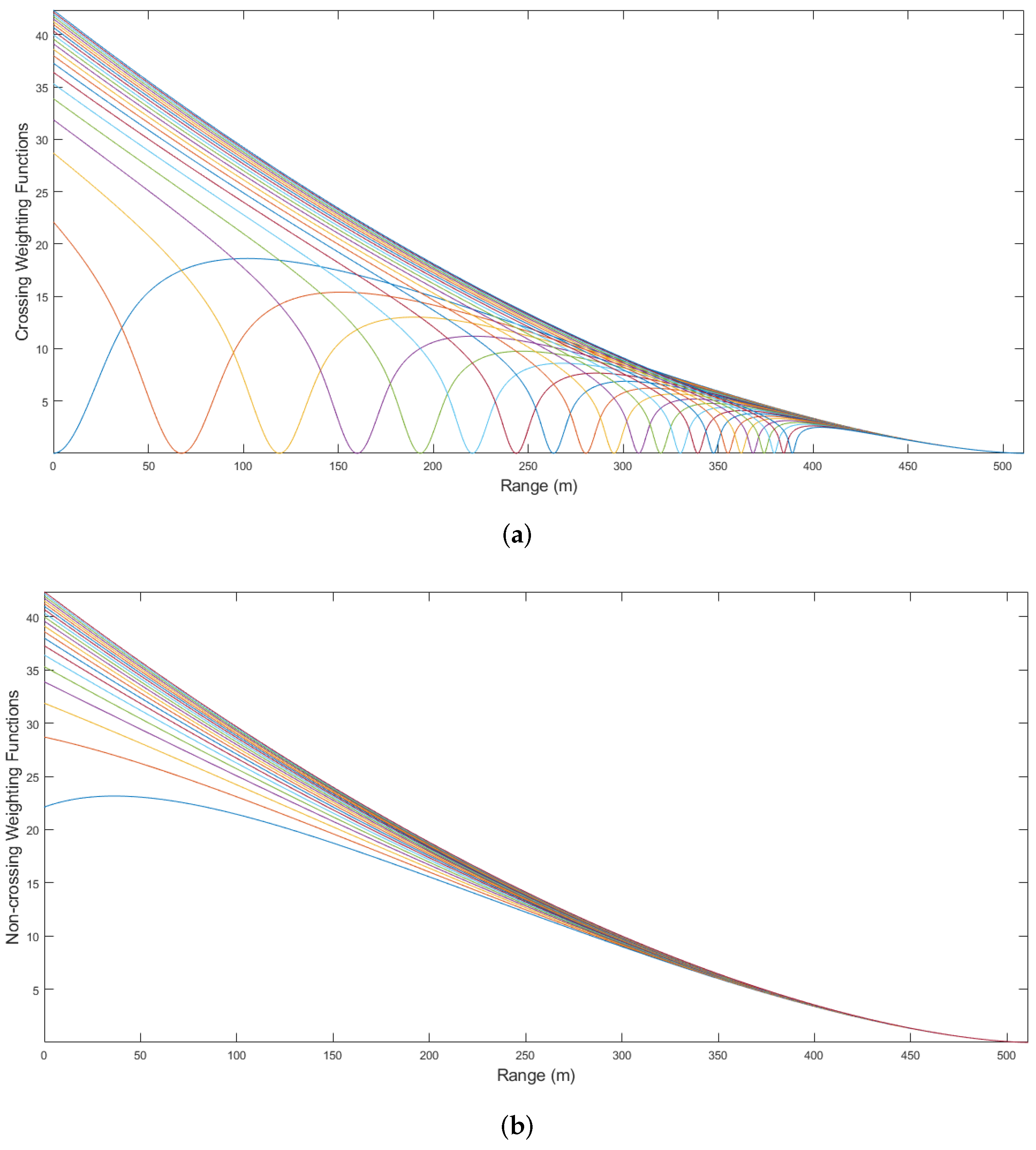
where s is now calculated for every subaperture separation from 1.67 cm to 35.09 cm. Unlike the crossing weighting functions, the lack of overlap along the sensing path in the non-crossing case ensures no points of zero influence. At the intersection points along the crossing paths, the turbulence contributions are equal and therefore do not affect the wavefront tilt measurement. The full set of weighting functions is shown in Figure 6.

Each of the weighting functions drops to zero at the source end of the path ($z=L$), which implies the turbulence near the laser beacons has little to no effect on the measured wavefront tilts [5]. The crossing weighting functions each have a notch along the path where their two sensing paths cross and the tilts cancel.

These 43 weighting functions are combined into a 43 × 1023 matrix, $\mathit{M}$, where each row is a separate weighting function and 1023 is the 511 m path discretized into 0.5 m increments. Given the weighting function matrix, an estimated $C_n^2$ profile over the path can be written as

$${\mathit{C}}_{n,est}^2={\mathit{M}}^{+}\mathit{V},$$

(3)

where ${\mathit{M}}^{+}$ is the Moore–Penrose pseudo-inverse of $\mathit{M}$ and $\mathit{V}$ is the matrix of differential tilt variances, each measured for the same subaperture separation as a corresponding weighting function. The pseudo-inverse calculation is thresholded such that singular values below a threshold are not inverted as another method of noise reduction. The ${\mathit{C}}_{\mathit{n},\mathit{est}}^{\mathit{2}}$ profile represents an estimate of the turbulence at each 0.5 m increment along the path. The chosen set of weighting functions are too similar past roughly 350 m to provide spatially distinct information and thus the profile breaks down past this point. 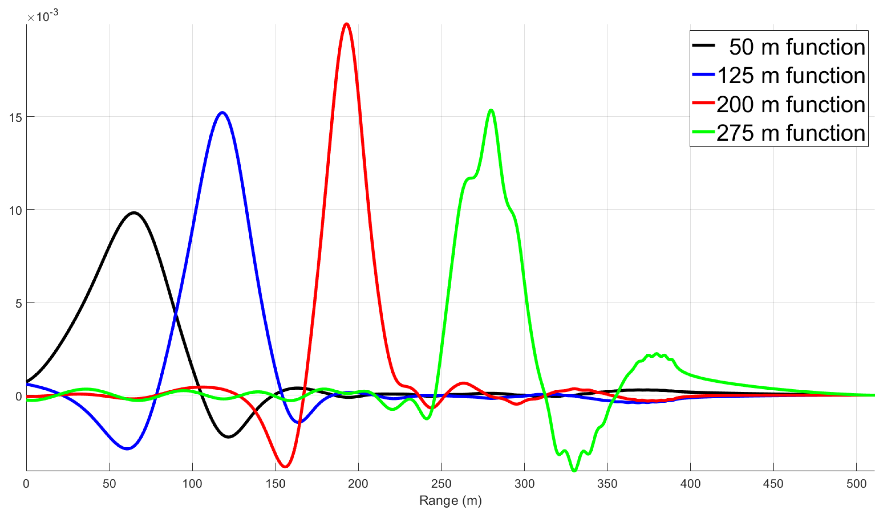The influence function, or impulse response matrix, is defined by ${\mathit{M}}^{+}\mathit{M}$ and describes how the point estimates of $C_n^2$ are affected by the distributed turbulence along the path. The influence functions at four locations are shown in Figure 7. This shows the evolution of the technique’s spatial resolution.

2.2. Tikhonov Regularization

Tikhonov regularization, also known as ridge regression, is a common strategy for solving ill-posed problems, which is the case for the weighting function matrix used here. This method improves the conditioning of the matrix by adding positive elements along its diagonal.

$${\mathit{C}}_{\mathit{n},\mathit{est}}^{\mathit{2}}={({\mathit{M}}^T\mathit{M}+{\mathsf{\Gamma }}^T\mathsf{\Gamma })}^{-1}{\mathit{M}}^T\mathit{V}.$$

(4)

$\mathsf{\Gamma }=\alpha \mathit{L}$ is the Tikhonov matrix, where $\alpha$ is the ridge parameter and $\mathit{L}$ is the identity matrix. Regularization is used as an improvement over the pseudo-inverse to calculate the $C_n^2$ profile. The ill-conditioned nature of the weighting function matrix makes it highly susceptible to measurement noise, which appears as dropouts in the profile (negative and therefore unphysical values of $C_n^2$). The pseudo-inverse is only able to eliminate these dropouts using higher thresholds, which removes the contribution of select weighting functions. Tikhonov regularization can instead be applied to solve the ill-conditioned problem by minimizing the solution and residual norms. The regularized solution, $\mathit{X}$, is determined by

$${\mathit{C}}_{\mathit{n},\mathit{est}}^{\mathit{2}}=argmin\left\{\left|\right|\mathit{M}\mathit{X}-{\mathit{V}\left|\right|}_2+{\alpha \left|\right|\mathit{X}\mathit{L}\left|\right|}_2\right\}.$$

(5)

The MATLAB constrained nonlinear optimizer function fmincon was used to find the minimum of Equation (5). Ridge parameter selection is informed using the L-curve method, which seeks the knee in a log-log plot of the regularized solution against the norm of its residual norm. The parameter nearest to the knee in the L-curve was used as the initial guess, which was then adjusted to eliminate $C_n^2$ dropouts from the profile while not over-regularizing the solution [18]. An example of the ridge parameter’s influence on the turbulence profile is shown in Figure 8.

3. Results

The following profiles are presented in UTC (4 h ahead of local time). The limitations on the weighting functions due to the sensing path geometry greatly reduce the reliability of the $C_n^2$ predictions after roughly 350 m in each profile. A threshold was used during the pseudoinverse calculation to further reduce measurement noise. The threshold value determined the limit such that smaller singular values of $\mathit{M}$ would not be inverted. This reduces the number of dropouts in the profile, where the noise causes the $C_n^2$ estimates to be negative and therefore unphysical. 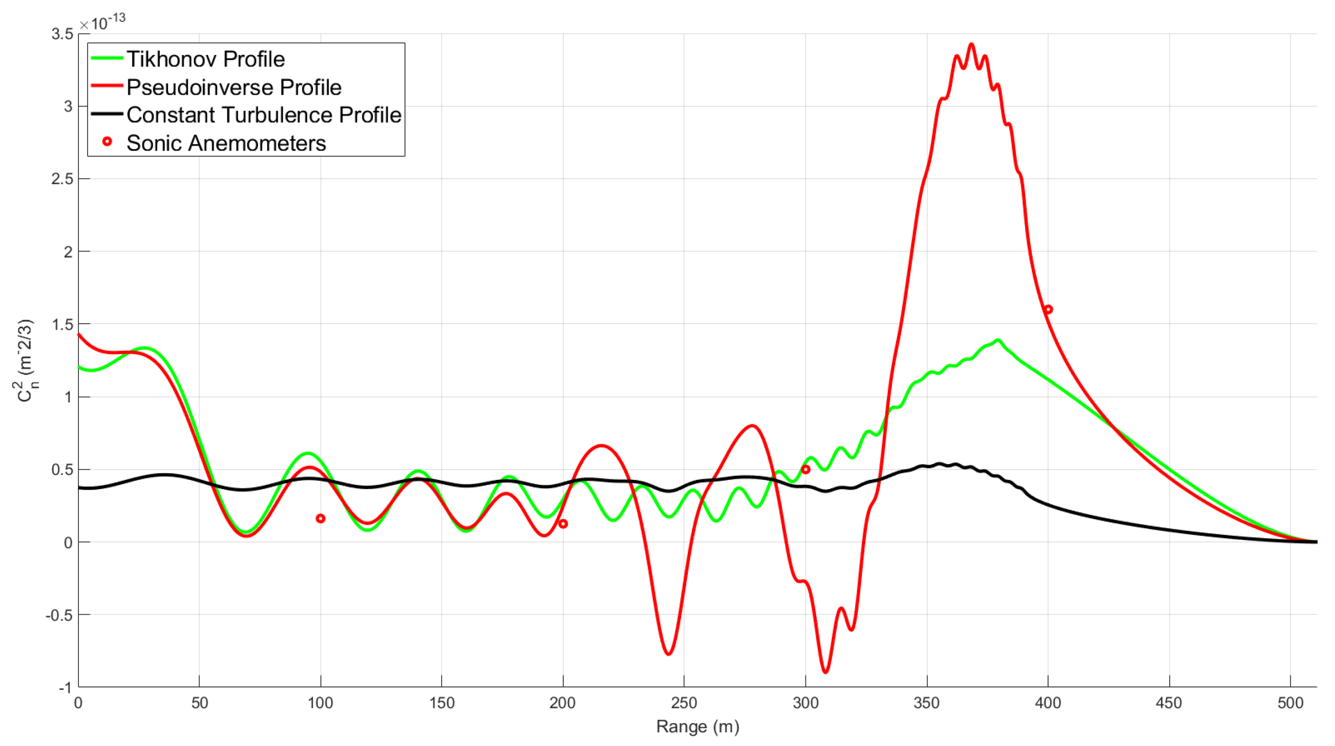Each of the following profiles used a pseudoinverse threshold of 35, which is $2.6\%$ of the largest singular value of the weighting function matrix. The spatial resolution of the results is set by the profiling technique and is not constant along the path. Past the final notch in Figure 6a, there is no spatial resolution. The resolution along the path is shown in Figure 9 by the constant turbulence case calculated by the BLS. The imaginary ripples in the constant $C_n^2$ case are noise due to the reconstruction technique and the limitations of the experimental setup (i.e., the number of available subapertures and their spacing).

4. Discussion

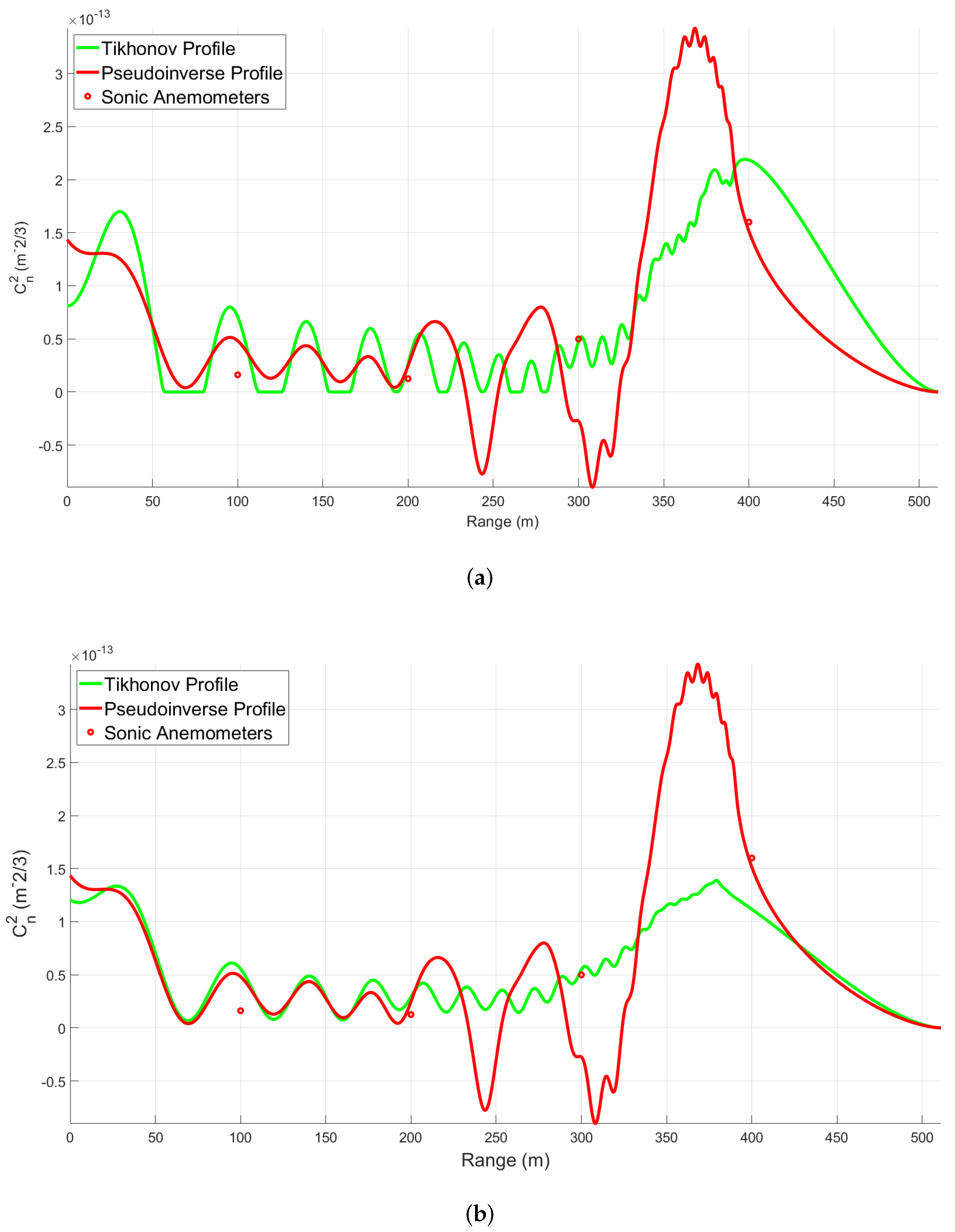
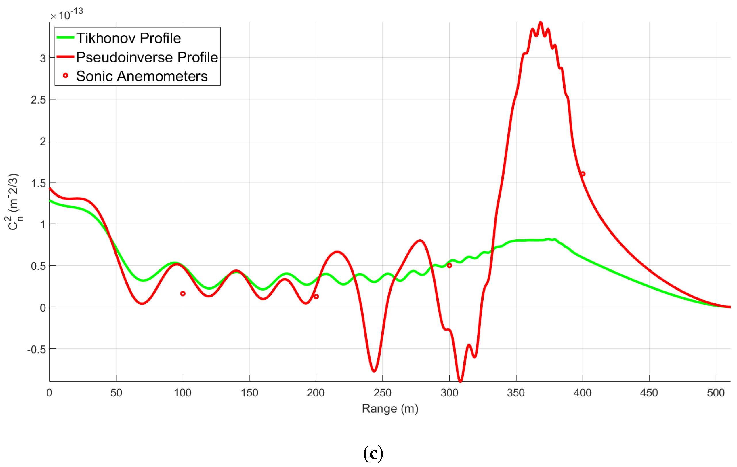
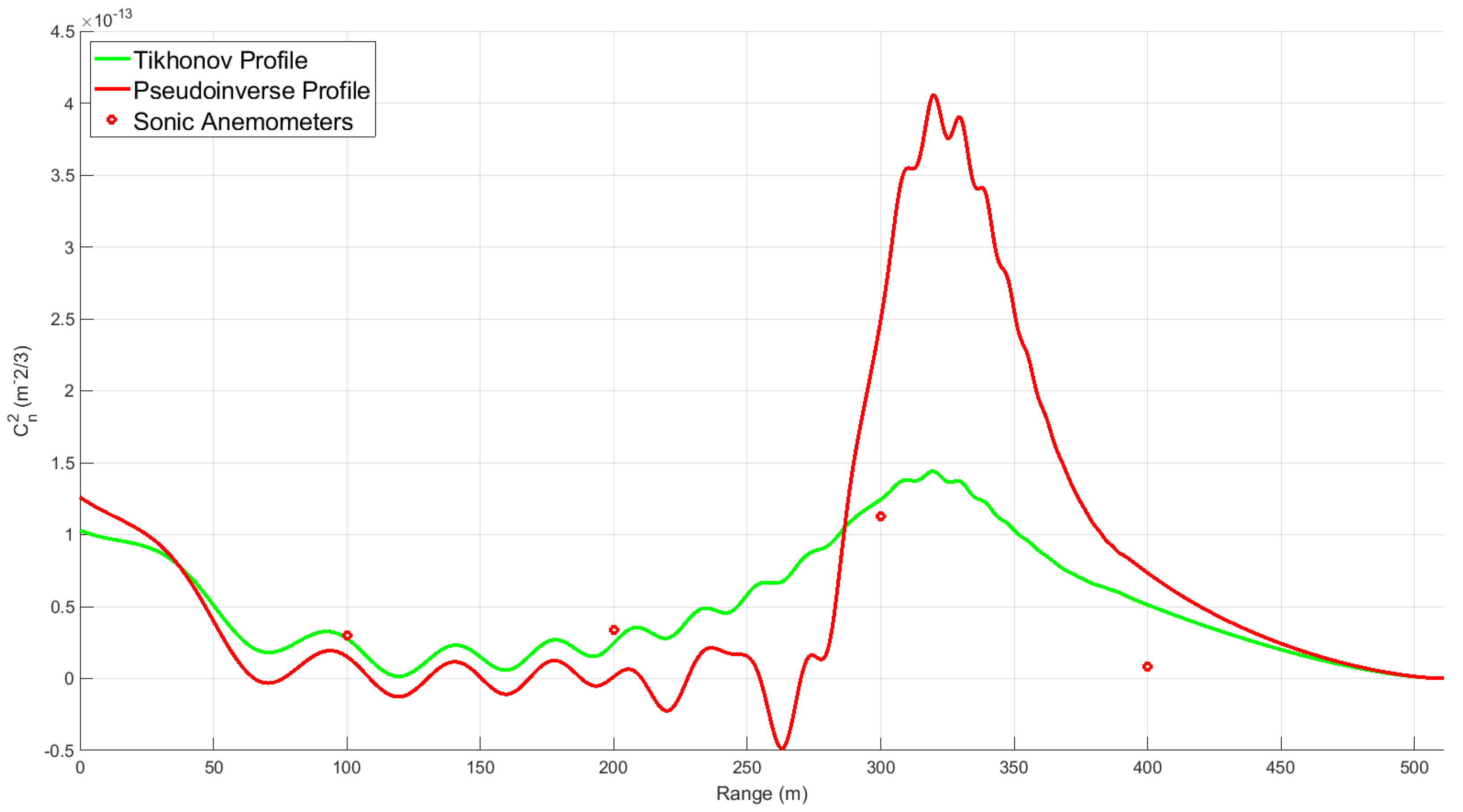
The profiles here show strong correlation between the Tikhonov regularized HTS profiles and the associated scintillometer and anemometer data. The pseudo-inverse profiles still show a significant amount of measurement noise, which causes large fluctuations and drop-outs in the profiles. The Tikhonov regularization is successfully able to reduce this noise and correct the profiles. Over the two days of data collection, values of $C_n^2$ between $9\times {10}^{-15}$ to $6\times {10}^{-13}$ m${}^{-2/3}$ were measured by the BLS. Periods of higher turbulence on the order of ${10}^{-13}$ m${}^{-2/3}$ produced less accurate profiles with greater noise. This may be due to the limitations of the centroid tracking method. The system used for this study tends to produce the best profiles during periods of moderate to weak turbulence around ${10}^{-14}$ m${}^{-2/3}$. The profiles accurately captured the predicted and anemometer measured rise in $C_n^2$ over the concrete portion of the path. In cases where the anemometers measured a drop in turbulence over the second half of the path, such as in Figure 10 past 300 m, the Tikhonov profiles accurately captured the dip. Given that the profiles always break down past 350 m, the anemometer at 400 m was not reliable for the sake of comparison, but was useful for observing the general turbulence trend along the path.

There are several challenges with this technique that affect its ability to generate profiles. Many data sets were unusable due to subimage misalignment, which made it impossible to track the centroid motion. Periods of strong turbulence also caused issues due to the subimages shifting outside of their respective tracking windows, thereby affecting the measurements of neighboring subimages. In these cases, the current auto-focusing algorithm was not able to properly track the centroid motions and could therefore not salvage the tilt variance information. These issues could be addressed in future work by a more advanced auto-focusing algorithm or a different optical design. Future work may also consider varied sensing paths. Elevating either the laser beacons or the HTS could provide $C_n^2$ profiles that give insight into the turbulence distribution as a function of height. The geometry of the sensing paths between the lasers and HTS subapertures cause the turbulence near the source end of the path to have very little effect on the tilt measurements. The impacts of this have not yet been explored, but could be addressed in future work by switching the placement of the lasers and HTS such that $z=0$ is over grass and $z=L$ is over concrete. Profile resolution near the apertures could be improved by decreasing the subaperture separations or increasing the separation of the source beacons. Varying these parameters to observe their effects on the profile is another topic for future work.

5. Conclusions

A method for estimating the turbulence profile over a horizontal path using a Hartmann Turbulence Sensor and two source beacons has been described. This method’s measurement technique is similar to SLODAR, but an entirely different methodology is used for turbulence profile reconstruction. Analytical expressions for the path weighting functions of crossing and non-crossing geometries have been shown to depend on subaperture size and separations, the separation of the source beacons, and the length of the sensing path. Each weighting function is constructed using varying subaperture separations. This gives them their unique shapes, which help with the pseudo-inversion process. The influence functions produced by these weighting functions suggest that the technique’s spatial resolution is highest near the HTS end of the path and steadily declines until the final weighting function notch location as shown in Figure 6a (roughly 350 m for this experimental setup). Past this point, the technique’s spatial resolution is effectively zero due to the lack of weighting function diversity.

This is a phase-based approach that is not prone to the saturation issues faced by irradiance-based techniques [5]. Therefore, this approach may be applied over greater sensing distances than others presuming similar aperture sizes. This methodology and analysis provide a deeper understanding of surface layer turbulence phenomena. This technique may prove to be an effective tool in long range imagery or directed energy through the atmosphere when used in conjunction with a multi-conjugate AO system.