Abstract
Marine pollution, which can cause damage to marine ecosystems, cut fishery production, and even harm human health, has aroused worldwide interest in recent years. Marine pollution reduction operations can stagnate in the case that the source of the pollution is unknown or hidden. In this paper, we present a novel method for marine pollution source localization using a network of mobile sensor nodes, such as autonomous underwater vehicles equipped with chemical sensors. Traditional reactive control methods can respond quickly to the shape dynamics of a chemical plume; however, they can hardly achieve intelligent cooperation unlike deliberative methods. In this study, we present a behavior composition method that attempts to combine the advantages of reactive and deliberative methods. An upwind-customized crossover operation based on the genetic algorithm was formulated as one of the elementary behaviors. The upwind sprint and movement away from the centroid of the sensor nodes were also modeled as another two elementary behaviors. Different sensor nodes are capable of different simultaneous elementary behaviors, enabling behavior composition in the mobile sensor network during plume source localization. The proposed method was evaluated using a widely used filamentous plume simulation platform, which has been used to facilitate field experiments in real marine environments. Simulation results indicate that the proposed method achieved high time-efficiency and localization accuracy during plume source localization in marine environments.
1. Introduction
As the worldwide industries develop rapidly, marine pollution is becoming increasingly serious [1]. Marine pollution can cause heavy damage to marine ecosystems, reduce the production of culture fisheries, and harm human health. One of the most common sources of marine pollution is the chemical sewage discharged by factories and ships into seas and oceans. Locating the sources of chemical contaminants is critical to reducing chemical pollution in marine environments, in which the transport of chemical materials is dominated by turbulences with a high Reynolds number [2]. The continuously released chemical materials in marine environments form meandering plumes with intermittent or patchy chemical distributions [3,4], which poses difficulties for static sensor nodes to detect the chemical pollution in a “wait-and-measure” manner. Furthermore, a network of static chemical sensing platforms/nodes, which is typically used for locating a chemical source in environments with low Reynolds numbers [5,6] or a fixed transportation network [7], cannot sense chemicals transported outside its limited coverage area. In contrast, mobile chemical sensing nodes [3,8,9,10,11], which are equipped with flow-velocity and chemical sensors, can theoretically cover an indefinitely large area if the power supply is guaranteed. This makes mobile sensing nodes more flexible and particularly suitable for locating chemical plume sources in large-scale marine environments. Moreover, multiple mobile sensor nodes (SNs) have higher robustness, stronger spatial sampling ability, and lower cost than a single mobile sensing robot/node, owing to the faculty of cooperation among multiple nodes [12]. Thus, the problem of locating a continuous chemical pollution source in marine environments though cooperation among a network of mobile sensor nodes is the focus in this paper.
To realize cooperation, a mobile sensor network (MSN) is defined as a wireless communication network that provides the infrastructure for sharing information among the SNs, with a designed cooperation scheme to control them. Existing methods for solving the chemical plume source localization (CPSL) problem using multiple SNs can be tentatively classified into deliberative and behavior-based methods. Deliberative methods, which select the best action by inferring, based on an implicit or explicit internal world representation [13], dominate existing multi-SN-based CPSL methods. Some recent typical deliberative and quasi-deliberative multi-SN-based CPSL methods are as follows. Hadi et al. [2] proposed an information theoretic search strategy in which a particle filter representation of the posterior source location belief distribution was employed to determine the robot’s actions. They also proposed a multi-agent collaborative “infotaxis” strategy [14], in which the rate of detecting the presence of a material plume is modeled as Poisson’s distribution. Yan et al. [15] proposed a modified convergence-guaranteed particle swarm optimizer method, in which the memorized particle optima, global optimum, and optimal group can be considered as a customized representation of the plume environment. Zhu [16] proposed a modified artificial potential field method that controls the robots to track the chemical plume based on the constructed source distribution probability model.
Compared with pure reactive methods, which tightly couple sensory inputs and effector outputs, deliberative methods are less sensitive to environmental dynamics [13]. However, pure reactive methods can stagnate in the absence of sensory inputs, which means they lack intelligence based on world representation. Behavior-based systems are best suited for dynamically changing environments, where a fast response and adaptivity, as well as the reasoning ability, are required [13]. In behavior-based methods, different SNs can simultaneously perform different and frequently switched elementary actions, enabling behavior composition [17] in the MSN. In the domain of multi-SN-based CPSL, the spiral-surge (SS) method proposed by Hayes et al. [18] is a typical behavior-composition method. On the one hand, SS controls the SN currently detecting above-threshold concentrations to move upwind. This is a typical reactive control method because the upwind sprint is directly activated when an odor-detection event occurs. On the other hand, SS employs a deterministic outward spiral movement to steer the SNs when the MSN does not detect any valid concentration information. Moreover, SS uses simple explicit binary communication signals to enable cooperation among the SNs [18]. By combining reactive behavior (i.e., upwind sprint), deterministic spiraling movement, and simple binary communication, the SS method achieves remarkable efficiency in cooperative chemical source localization. However, combining reactive behaviors and intelligent deliberative methods in cooperative CPSL processes requires further investigation.
In this paper, we proposed an upwind-adapted genetic algorithm (uGA) that combines the upwind-adapted crossover operator based on the genetic algorithm (GA) [19,20] and the reactive upwind sprint. The GA is an intelligent optimization algorithm that is traditionally used to search for the global maximum of a fitness function. Empirically, there are some lasting but wandering concentration maxima near the chemical-release source. By searching for the concentration maxima, the GA and other optimization algorithms can be used to solve the CPSL problem. However, unlike the direct calculation of fitness values in numerical optimizations, SNs equipped with common chemical sensors should arrive at an objective location to detect the concentration. It is difficult for SNs to obtain essential concentration detection owing to the intermittent and dynamic distribution of chemicals. Moreover, some local concentration maxima exist at significant distances from the plume source [3]. Thus, solving the CPSL problem is not straightforward.
To overcome these difficulties, the uGA attempts to combine the advantages of reactive upwind sprints and an upwind-customized crossover operation based on the GA as follows. First, a customized crossover operator is modeled as the elementary C-behavior. The crossover operator in the GA is customized by restricting the newly generated chromosome to the upwind search area of the chromosome centroid. Second, for an individual SN, the upwind sprint and a deterministic departure from the SN centroid are modeled as elementary U-behavior and D-behavior, respectively. Third, with respect to the different situations in the CPSL process, the three elementary behaviors are combined to form two combinational behaviors. The most commonly used filamentous plume simulation platform (FPSP) [9], which was proposed to assist field experiments by Farrell et al. [21], was employed here to compare the performance of the proposed uGA method and the SS method. It is expected that using uGA in the MSN-based CPSL problem can improve the time-efficiency of the CPSL process, which is significant for reducing the loss caused by the targeted pollution.
2. Combining Upwind Sprint and GA for CPSL
2.1. Original GA
To reveal the adaptations made on the GA, the original form of GA is introduced first. Algorithm 1 shows the pseudocodes of GA. As a population-based algorithm, the population of GA comprises m individuals, which are encoded into strings of binary numbers. In other words, the size of the GA population is denoted as m, i.e., GA maintains a population of m chromosomes [19]. At the initialization stage, the m chromosomes are randomly generated in the whole search space. For traditional function optimization problems, the search space is defined by the argument domains of the fitness function.
| Algorithm 1. Original GA [20]. |
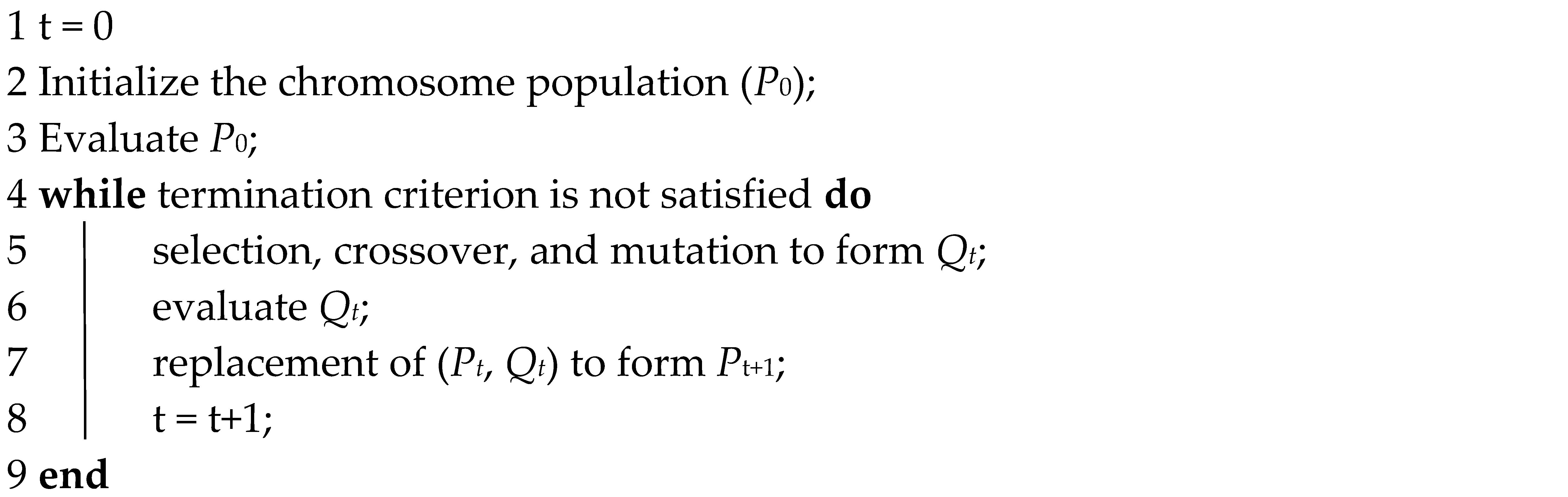 |
After initialization, all solutions are evaluated by substituting them into the fitness function and calculating the corresponding fitness values. The GA then enters an iterative loop, in which every iterative cycle has three typical operators: selection, crossover, and mutation. For the crossover operators, the selection operator selects m × pc chromosomes by following a fitness-based roulette-wheel selection rule. Chromosomes corresponding to larger fitness values during the selection process are more likely to be selected than those with smaller fitness values. To depreciate the chromosomes with small fitness-values, a novel fitness function was proposed for function minimization problems by Xin et al. [22], as follows:
in which y is the objective function; b is the minimum objective value at the t-th cycle; and
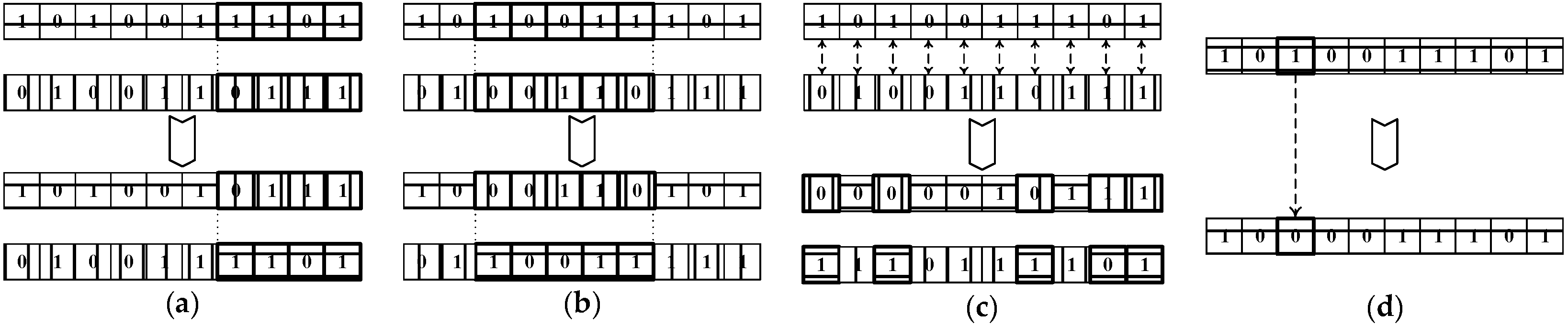
Four typical crossover operators [23] are illustrated in Figure 1, in which alleles in bold squares are changed in the operators. In the uniform crossover, all the alleles are switched at the same probability of 0.5. After the crossover operation, the mutation operation is conducted on the new chromosome. As shown in Figure 1d, one of the alleles in the new chromosome is inverted at a probability of pm [23].

Figure 1.
Typical crossover and mutation operators in the GA. Changed alleles are indicated using bold squares. (a) One-point crossover; (b) two-point crossover; (c) uniform crossover; (d) mutation.
After crossover and mutation, the fitness values of new chromosomes are evaluated by decoding and substituting them into the fitness function. If the fitness value of the new chromosome is higher than that of the old chromosome, it is inserted into the population and replaced by the old one. The termination criterion is verified at each iteration loop. If the termination criterion is not satisfied, the iterative loop is repeated. Typically, when t exceeds a predefined maximum cycle number, GA is terminated.
2.2. Adapting GA for CPSL
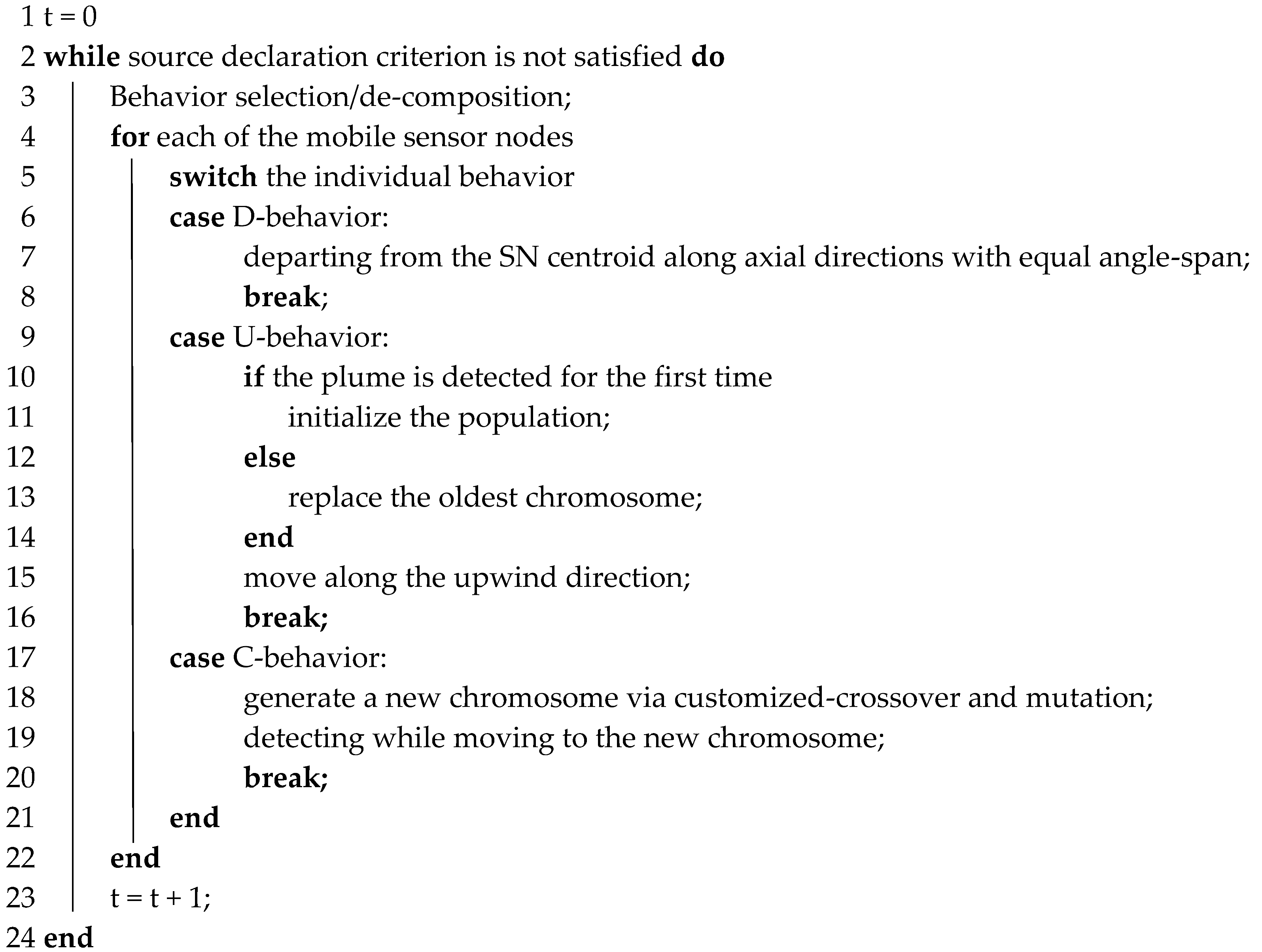
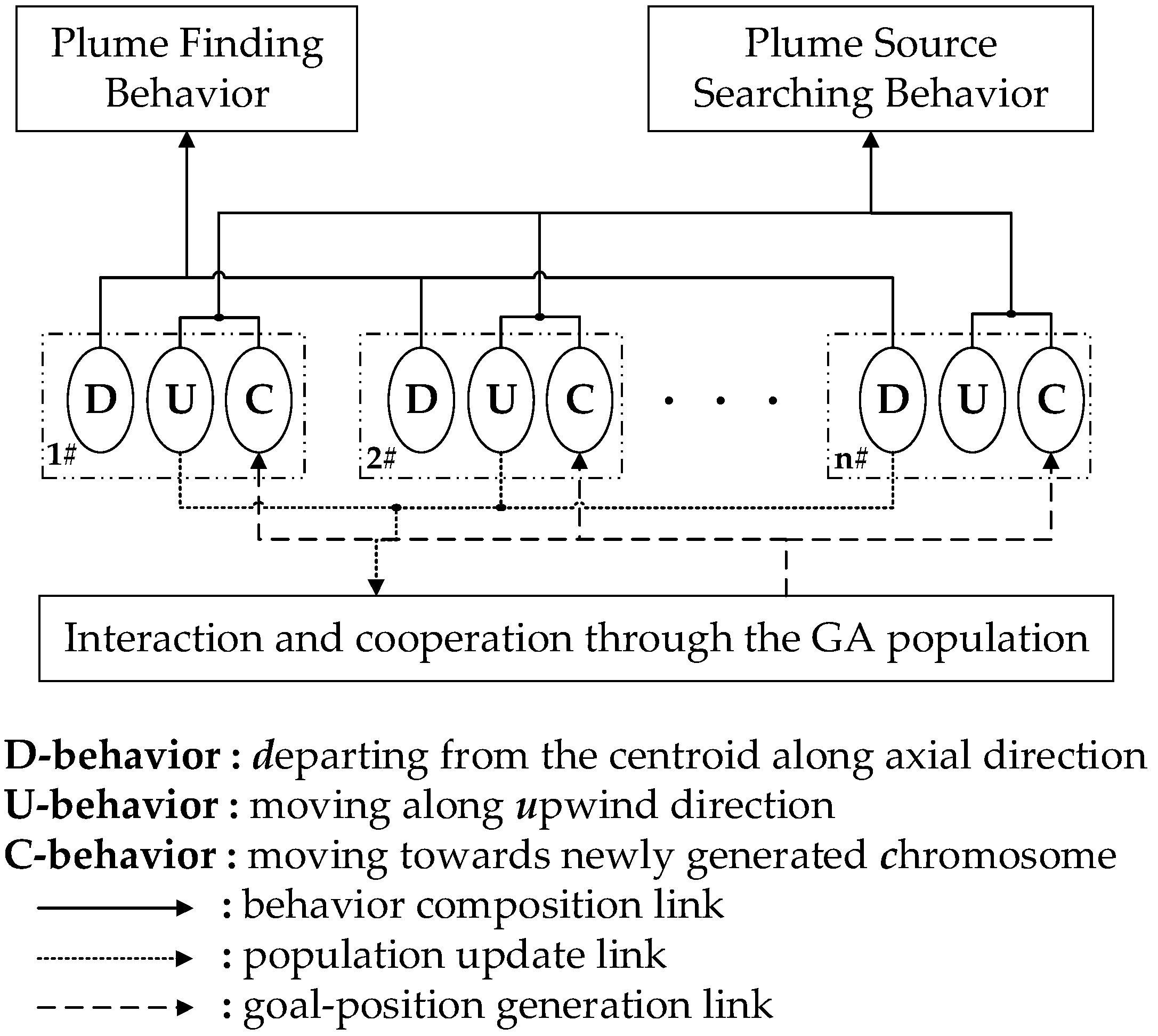
The structure and pseudocodes of the uGA method are shown in Figure 2 and Algorithm 2, respectively. In Figure 2, two compositional behaviors are exhibited in the top layer: plume finding and pollution source searching. The compositional behaviors comprise elementary behaviors in the middle layer, namely D-behavior, U-behavior, and C-behavior, which correspond with the three cases in Algorithm 2.

Figure 2.
Structure of the uGA method.
| Algorithm 2 uGA. |
 |
2.2.1. Behavior Selection Scheme
As depicted in Figure 2, the plume-finding behavior comprises the D-behaviors of all SNs, whereas the pollution source searching behavior comprises U-behaviors and C-behaviors. In other words, all SNs conduct the D-behavior when the plume-finding/re-finding behavior is activated, whereas U-behavior and C-behavior are candidate elementary behaviors for the SNs when pollution source searching behavior is activated.
For behavior selection, two time-cycle thresholds are defined: lldi (where i = 1, 2, …, n) and gld. lldi is the time-cycle duration since the i-th SN obtained an above-threshold concentration measurement until the present. gld is the time-cycle duration since the last above-threshold concentration measurement of the MSN until the present. Thus, the value of gld can be calculated as
Moreover, thl, tha, and thf are three predefined time-cycle thresholds that satisfy thl < tha < thf, where thl is a small number. lldi < thl means the i-th SNs are still moving inside of the plume profile. At the k-th cycle time, the activated compositional behavior and the elementary behavior activated for the i-th SNs are denoted as B and , respectively. The behavior selection scheme of the uGA, which corresponds with line 3 in Algorithm 2, can be represented as follows.
According to Equations (4) and (5), the circumstance of the MSN is classified as gld < thl, thl < gld < tha, and tha ≤ gld < thm and gld equals thm:
- (1)
- gld < thl: At least one SN is currently keeping in contact with the plume. In this circumstance, as a cooperation mechanism, the newly detected plume information can be exploited by the SNs.
- (2)
- thl < gld < tha: All n SNs have lost contact with the plume. However, the previously detected information is still time-efficient and can be exploited to recontact the plume.
- (3)
- tha ≤ gld < thm: All n SNs have lost contact with the plume for a long time. It is necessary to explore the uncovered search space for recontacting the plume.
- (4)
- gld equals thm: The CPSL process is considered as failed.
2.2.2. Elementary Behaviors
Aiming at the above-mentioned circumstance of the MSN, elementary behaviors are designed for individual SNs. Different SNs can simultaneously perform different elementary behaviors.
- D-behavior: The SN moves away from the centroid of the MSN with the perspective of exploring the uncovered space. In the D-behavior, the goal position of the i-th SN with coordinates {xgi, ygi} iswhere xc and yc are the x- and y-coordinates of the MSN centroid, respectively, and n is the number of SNs in the MSN. The goal positions in Equation (6) can guide the SNs to move along radial directions with equal angle-spans.
- U-behavior: The SN moves in the opposite direction to that of the detected fluid-flow to search in the upwind area. The upwind movement direction angle can be denoted as θi = π + βi, where βi is the flow direction angle detected by the i-th SN.
- C-behavior: The SN moves toward the new candidate chromosome generated by the GA to evaluate it. Once the C-behavior is performed, a new chromosome is generated by conducting crossover operation on the GA population.
As underlined in Algorithm 2, the GA-correlated operations in uGA include initialization, population update, candidate chromosome generation and evaluation, and the termination criterion.
- Initialization (line 8 in Algorithm 2).
When the MSN encounters the first contact with the chemical plume, m new chromosomes are randomly initialized in the neighborhood of the position of the first contact. The concentration measured at the first contact is substituted into Equation (7) to calculate the objective value of the initial chromosomes.
in which y and z are the objective value and detected concentration, respectively.
- 2.
- Population update (line 10 in Algorithm 2).
If the SNs detect a new above-threshold concentration in the upwind area of the population centroid, the detection position is encoded to a new chromosome and then inserted into the population. To maintain a fixed population size, which is denoted as m, the oldest chromosome in the population is discarded after the new chromosome is inserted. In other words, the oldest chromosome is replaced by the newest chromosome and the population is updated in a first-in-first-out manner.
- 3.
- Candidate chromosome generation (line 15 in Algorithm 2).
Once C-behavior is activated, only one candidate chromosome is generated by a crossover between the two selected chromosomes. The predefined parameters pc of GA is not used in uGA. To select chromosomes for the subsequent crossover operator, fitness-based roulette wheel selection is conducted based on the fitness function in Equation (1). The fitness value is calculated by substituting the result of Equation (7) into Equation (1), which was originally used for function minimization. Thus, the chromosome correlated with high concentration measurements is more likely to be selected in the roulette wheel selection.
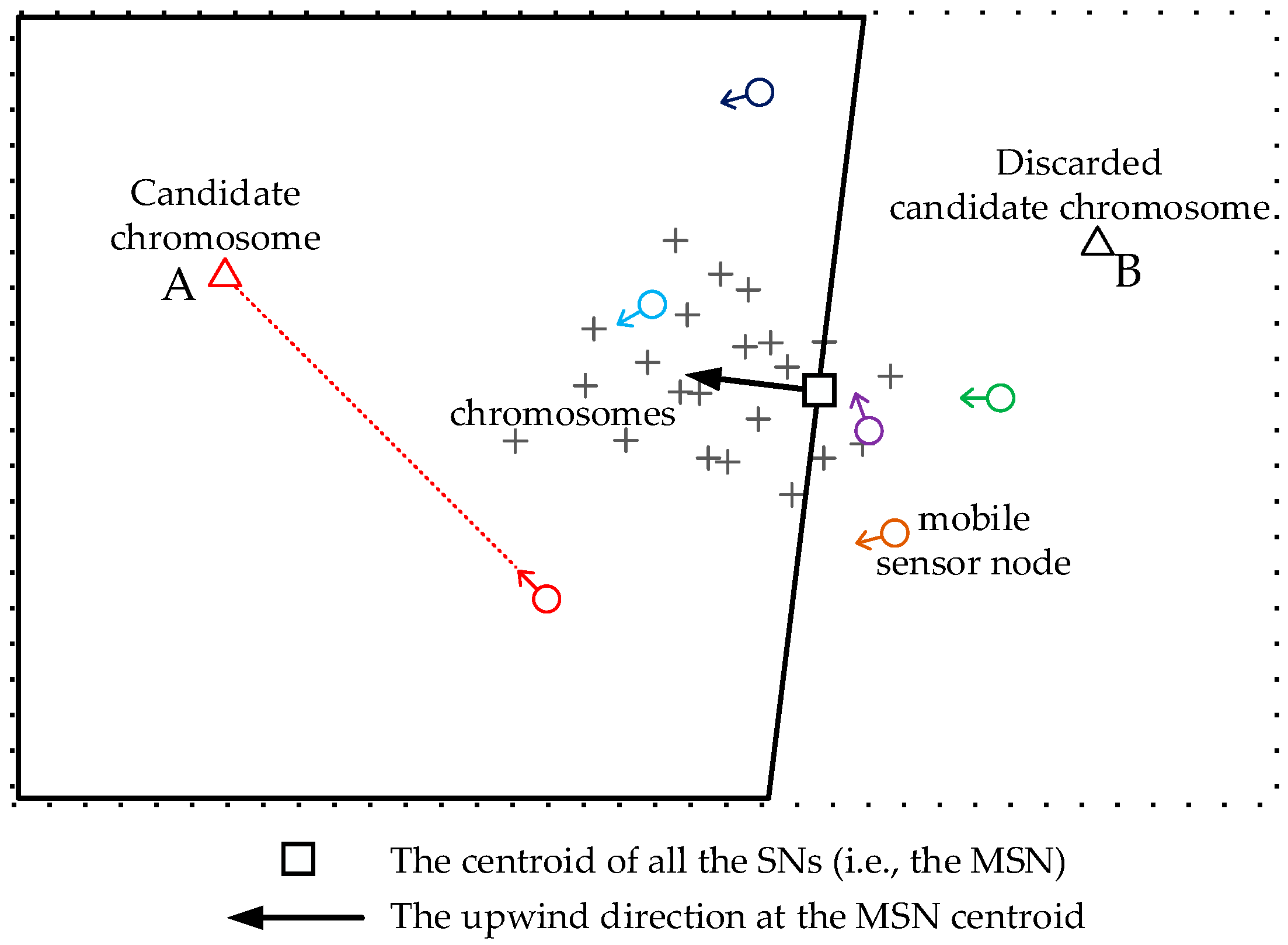
As illustrated in Figure 3, an additional condition is set up to filter the new chromosome. The additional condition is that newly generated chromosomes must be located in the upwind search area of the MSN centroid. If the condition is not satisfied, the selection and crossover processes should be repeated. The improved crossover is called upwind-customized crossover. For example, since position B lies in the subarea on the downwind side of the MSN centroid, the generated chromosome at B should be discarded. If the newly generated candidate chromosome falls inside the subarea on the upwind side of the sensor node centroid, such as position A, it will be retained as the new candidate chromosome for further evaluation. After the upwind-customized crossover operation, the mutation operation is conducted on the new chromosome.
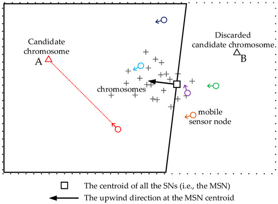
Figure 3.
The illustration of the customized crossover operator. The polygon with solid borderlines and the rectangle with dotted borderlines are the upwind search area and the whole search area, respectively.
- 4.
- Candidate chromosome evaluation (line 16 in Algorithm 2).
To evaluate the newly generated candidate chromosome, an SN conducting C-behavior is steered to approach it. If the SN encounters an above-threshold concentration measurement on its way to the candidate chromosome, the evaluation process is terminated. Subsequently, the U-behavior and population update processes are activated.
- 5.
- Termination criterion (line 2 in Algorithm 2).
The position where the SN loses contact with the plume, denoted as the last contact position (LCP), is used to terminate the localization process. If the distance between successive LCPs does not exceed 1 m for 10 iterations, which means the LCPs converged at the newest LCP, then the uGA is terminated. The newest LCP is considered as the source location of the unknown chemical plume.
The differences between GA and uGA are summarized in Table 1.

Table 1.
Differences between GA and uGA.
3. Simulation Setup
The FPSP proposed by Farrell et al. [21] is used to test the proposed method. In FPSP, a 100 m-by-100 m square search area is simulated. Within the search area, six mobile sensor nodes are moving at a speed of 2 m/s to search for an unknown chemical plume source. From the source, a large number of chemical filaments that contain chemical material normally distributed relative to the filament center are continuously released and dispersed in the search area. Then, the released filaments are horizontally transferred by the dynamic turbulent flow. All released filaments contribute to the instantaneous concentration C(x, t) at x as follows [21]:
where N is the total number of filaments, Q is the amount of chemical substance units in a filament, and Ri(t) and piare the size parameter and position of the i-th filament, respectively. Typical values of Q and Ri(t) can be set as 8.3 × 10⁹ and , respectively [21]. It can be seen that the value of Ci(x,t) is dominated by Ri(t) and pi, which are influenced by the motion of the ith filament.
In the FPSP, the motion speed of the filaments is governed by the surrounding flow’s velocities. The degree of the flow velocity fluctuation, which can be changed by tuning the noise parameters a, b, and G [21], is positively correlated with the degree of variation in the filament’s positions. To complicate the CPSL problem, large-amplitude flow fluctuations [21] are generated by setting the parameters a, b, and G to 0.04, 0.04, and 20, respectively. Moreover, as a further development of FPSP, the time-varying flow velocities are saved to a file in chronological order.
Based on the same flow-velocity file, the SS method [17] is tested as a counterpart method for comparison with the uGA. The similarities and differences between the SS and uGA methods are summarized in Table 2. There are substantial differences between the SS and uGA methods, although both methods employ reactive upwind sprint operation to control the SN node currently in contact with the plume. First, in the plume reacquiring stage, SS and uGA steer the SNs along deterministic spiraling paths and toward the newly generated chromosome, respectively. Second, SS and uGA realize cooperation among the SNs through simple explicit “ATTRACT” communication and customized crossover of the genetic algorithm chromosomes, respectively. Third, as the termination condition, SS compares a predefined constant with the distance from the chemical source to the SNs, while the uGA uses the distances between successive LCPs to judge whether the SN locations converge. Because the plume source location is previously unknown in real CPSL applications, the calculation of the SN–source distance is not applicable.
Table 2.
Similarity and differences between the SS and uGA methods.
To test the uGA and SS methods under identical conditions in all trials, three setups were created, as follows:
- The same flow field was reproduced by periodically reading a file in which time-varying flow velocities were previously saved. This setup can help to avoid the influence of different flow fluctuations on the localization processes and results.
- The same plume-finding scheme was used, in which the MSN starts from the same rendezvous (the top-right corner) and departs from it along prefixed angles. In other words, the initial plume-finding stage, which is strongly influenced by the selection of the starting rendezvous, was not studied in these comparison simulations. Because of this setup, the parameter SpiralGap1 in the plume-finding stage of the original SS is omitted. Only the value of SpiralGap2 should be set in the SS simulations. For testing the FPSP, the value of SpiralGap2 was empirically set to 5 m.
- The same termination criterion was used to terminate the methods. The LCP convergence condition in uGA (i.e., the distance between successive LCPs did not exceed 1 meter for 10 LCPs) was also used to terminate SS.
4. Results and Discussion
4.1. Parameter Selection
There are five parameters in the uGA: population size m; mutation probability pm; and three time-cycle thresholds, thl, tha, and thm that satisfy thl < tha < thm. The values of thl and thm were empirically set as 5 and 5000, respectively. In the cases that gld > 5 and gld > 5000, it is reasonable to declare that the SN has lost contact with the plume and the CPSL process has failed, respectively. Moreover, to investigate the influence of the crossover operation on the performance of uGA, an additional variable is considered in the simulation: the crossover type, denoted as cTy. The cases cTy = 1, 2, and 3 mean that the one-point crossover, two-point crossover, and uniform crossover are employed in uGA, respectively. Therefore, the values of m, pm, tha, and cTy should be selected for subsequent simulations.
To efficiently determine the optimal value combination of m, tha, cTy, and pm, the orthogonal experimental design method [24] was used. The parameters m, tha, cTy, and pm were taken as orthogonal experimental factors, such that m ϵ {10, 20, 30}, tha ϵ {20, 40, 60}, cTy ϵ {1, 2, 3}, and pm ϵ {0.3, 0.5, 0.8}, respectively. There are nine different value combinations in the L9(34) orthogonal experiments. With respect to each value combination, the results of 20 simulation trials were recorded and averaged. Table 3 presents the average results.
Table 3.
Orthogonal experimental results of different m, tha, cTy, and pm in uGA.
The small localization errors in Table 3 indicate that the termination criterion of uGA can successfully declare the chemical source in the FPSP. Empirically, if the distance between the real and localized pollution source positions is smaller than 1 m, the SN can easily find the real pollution source when it arrives at the localization position-result. Moreover, the differences among the localization errors are minor when the values of m, tha, cTy, and pm vary within the 16 different value combinations. This is because the localization result is determined by the termination criterion, which is fixed to the same value for the different simulations in Table 3. Thus, the localization results are hardly influenced by the different parameter values of uGA.
However, the spent cycles, that is, the number of time cycles spent by the MSN from the beginning to termination, are prominently influenced by four orthogonal experimental factors. This is mainly because the values of m, tha, cTy, and pm can influence the degrees of exploitation and exploration in uGA. The value of m defines the length of the memorized detection points that are exploited by the C-behavior. tha and cTy determine the time-span and manner of exploiting memorized information. pm has a positive impact on the exploration ability of uGA. The value combination {m, tha, cTy, pm} = {20, 20, 2, 0.8}, which obtained the minimal averages and standard deviations (std) of the spent cycles in Table 2, is used for the following comparison experiments.
4.2. Results Comparison
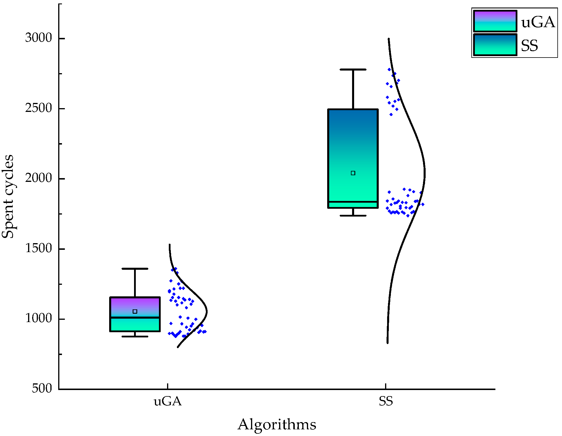
To statistically evaluate the performance of the uGA and SS methods, each of the two methods was tried 50 times. Figure 4 shows box plots of the time cycles spent in the 100 trials. The results in Figure 4 can be summarized as follows:

Figure 4.
Box plots of the time cycles spent by the uGA and SS methods. Each box plot is based on the results of 50 trials.
- (1)
- The average spent time cycles of uGA and SS are 1054 and 2041, respectively.
- (2)
- The spent time cycles of uGA are generally smaller than those of SS.
- (3)
- The distribution of the uGA time cycles is close to the normal distribution, whereas those of SS fall into two separate sectors that are far from each other.
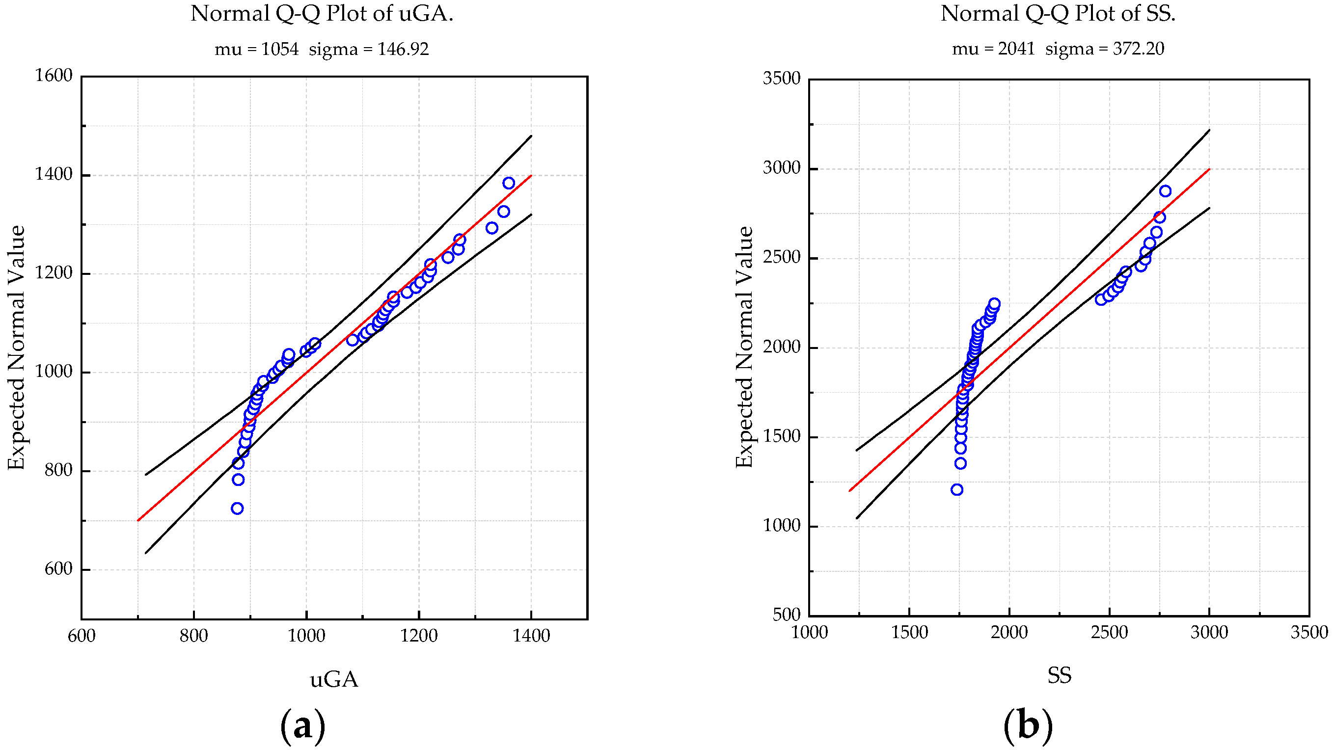
The quantile–quantile (Q–Q) plots in Figure 5 show the distance between the distribution of spent time cycles and the normal distribution. Almost all the points in Figure 5a lie within the area between the upper and lower percentile lines with a confidence level of 95%, which are close to the centerline y = x. In Figure 5b, there are only a few points between the two percentile lines. To some extent, the quasi-normal distribution of the time cycles spent by the uGA verifies that the localization efficiency of the uGA is stable in the dynamic flow field of the FPSP.
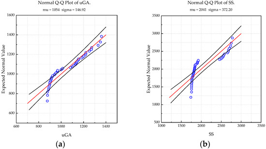
Figure 5.
Quantile–quantile (Q–Q) plots of the time cycles spent by uGA and SS. The thin gray lines are the upper and lower percentile lines with a confidence level of 95%. (a) Normal Q–Q plot of the time cycles spent by uGA; (b) normal Q–Q plot of the time cycles spent by SS.
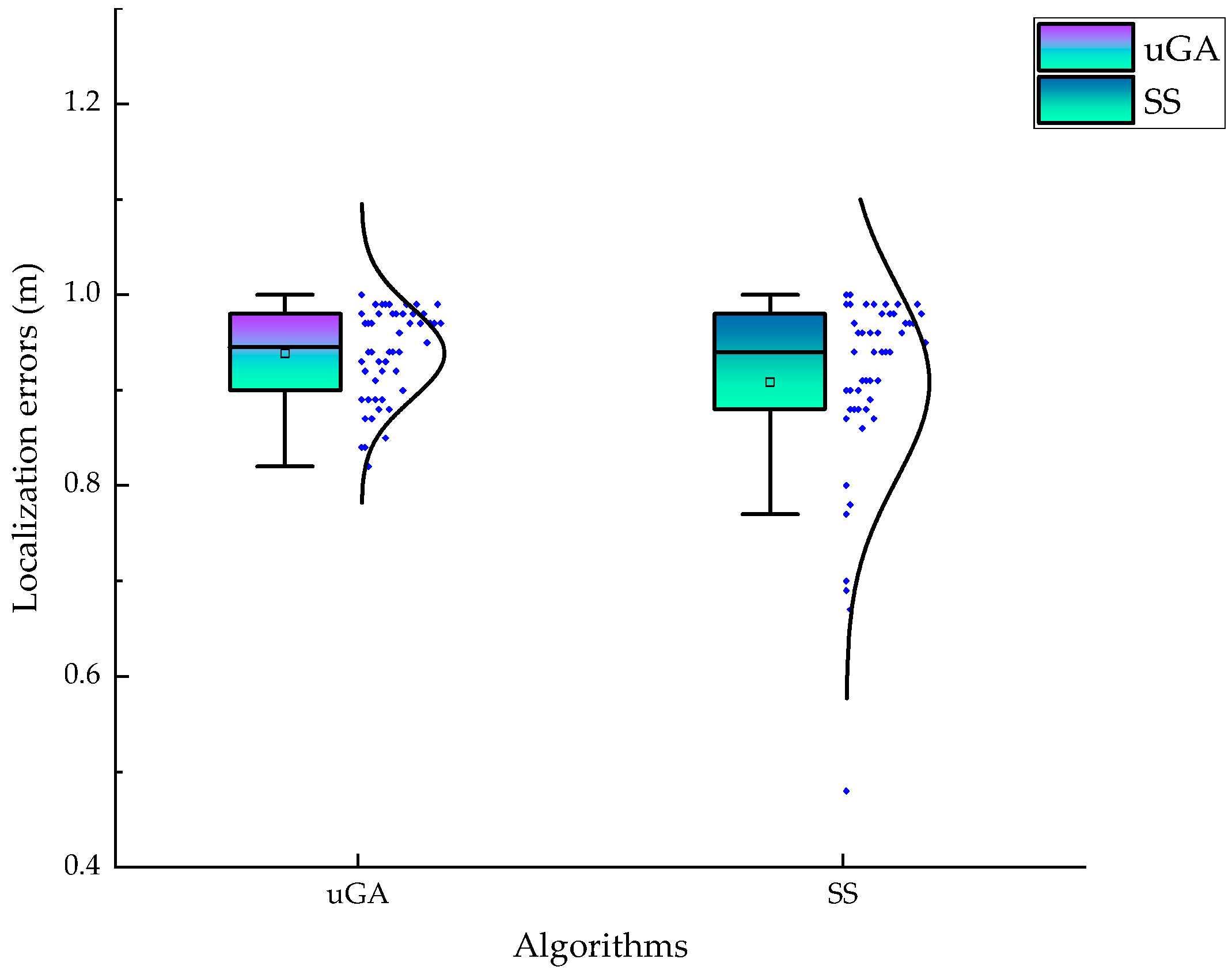
Apart from the localization efficiency, the localization error is another factor that should be considered in CPSL applications. Figure 6 shows box plots of the localization errors obtained using uGA and SS. In Figure 6, all the localization errors are smaller than 1.0 m, which means that it is easy to find the real chemical source within the neighborhood of all convergence locations. To summarize, the localization results verify that the termination criteria in uGA can successfully declare the chemical source in the FPSP.
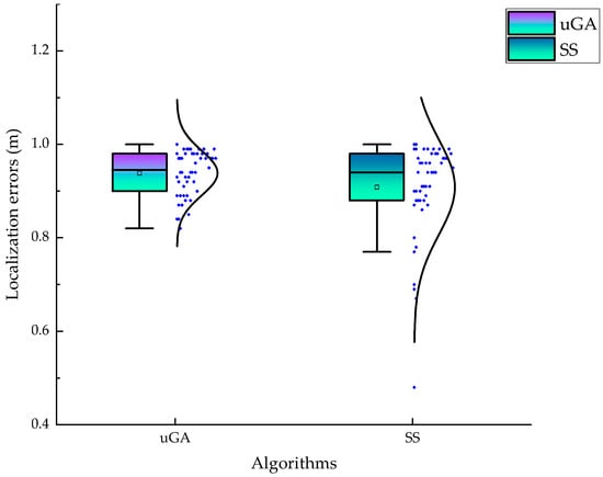
Figure 6.
Box plots of the localization errors obtained by the uGA and SS methods. Each box plot is based on the results of 50 trials.
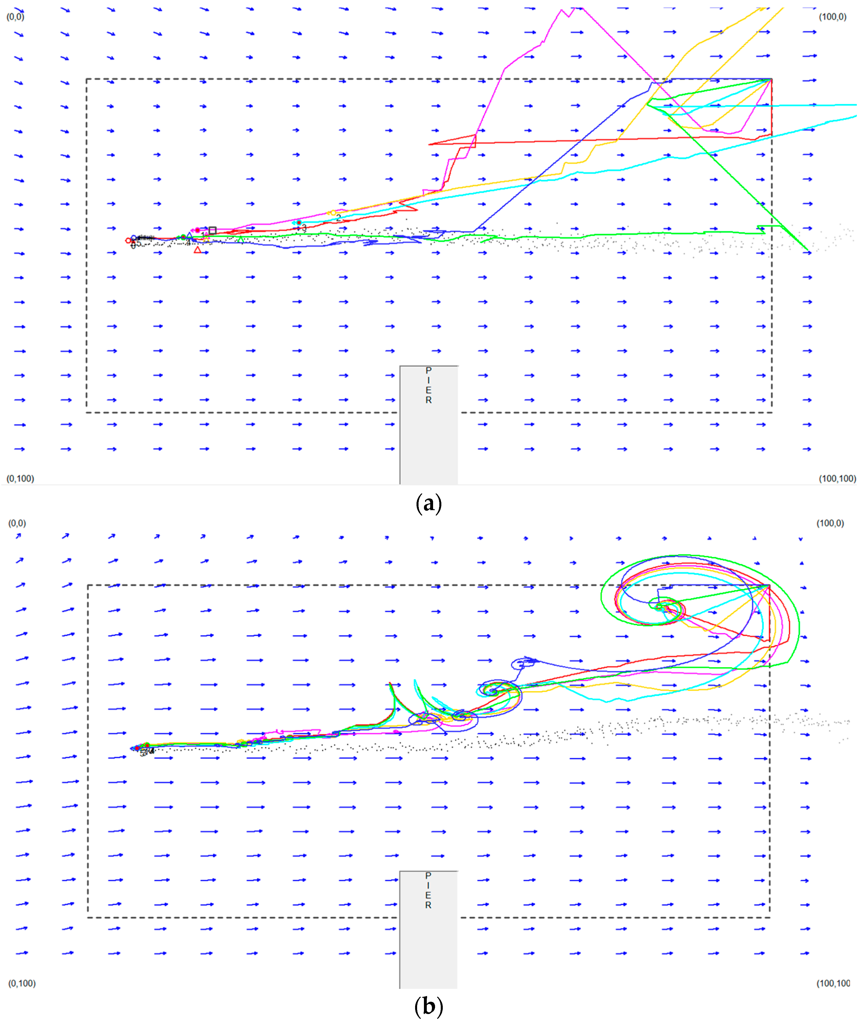
The moving paths of the SNs obtained when SS and uGA were employed are also compared. Figure 7 shows the paths generated in two typical simulation trials. In both trials, the MSN obtained its first contact with the plume at the top-right corner. When the SNs lost contact with the chemical plume, the plume re-finding behavior and spiraling movement were activated in uGA and SS, respectively. The paths in Figure 7 can be summarized as follows:
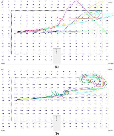
Figure 7.
Typical paths generated by the uGA and SS methods. Paths in different colors belong to different SNs. (a) Typical paths of the uGA method; (b) typical paths of the SS method.
- (1)
- The uGA outputs a set of straight-line paths, whereas the SS outputs revolving-shaped paths.
- (2)
- The interactions within the MSN in uGA were more effective than those in SS.
- (3)
The straight-line paths generated by uGA helped in reducing the path length for reacquiring the plume, since the shortest distance between two points is a straight line. Moreover, the SNs interacted with each other in SS through simple “ATRRACT” communications, whereas uGA enabled interaction within the MSN by the customized crossover operator in the C-behavior. The customized crossover operator is capable of improving the effectiveness by steering the SNs toward the upwind area of the MSN. In comparison, following one of the SNs via the ATTRACT communication in SS can only strengthen the contact between the MSN and the plume. Finally, after the SNs entered the left part of the search space, the diversity of the SN positions was well maintained by the D-behavior of uGA. Maintaining a relatively high SN diversity can help increase the area covered by the SNs and increase the probability of reacquiring the plume.
5. Conclusions
A behavior composition method, namely the uGA method, is proposed to solve the MSN-based CPSL problem. uGA combines the effectiveness of the reactive upwind sprint and the cooperative mechanism of the GA-based deliberative cooperation. Compared with the attraction mechanism used in the SS method, the C-behavior of uGA has two advantages. First, rather than just following the SN closest to the plume source, the new chromosome generated by the C-behavior of uGA is more likely to be closer to the plume source than all the current SN positions. Second, the C-behavior can help maintain the diversity of the SN positions, while the SN diversity is severely reduced when other SNs get close to the SN attracting them. Moreover, the D-behavior can further improve the search efficiency by increasing the diversity of SN positions.
Simulation results show that the proposed uGA method achieved high efficiency during plume source localization in simulated marine environments. Considering CPSL processes are often started after the pollution material is previously encountered, which facilitates the setup of a downwind start position for the MSN, all SNs started from the downwind side of the simulated pollution source. The case that the SNs started at the upwind area of the pollution source may cause the calculation time to increase. Moreover, inaccurate measurements or transmission mistakes may cause the localization accuracy and efficiency to decrease. Further research lines include: (1) designing new behaviors for better maintaining the SN diversity and striking a balance between plume information exploration and exploitation; (2) conducting field experiments using autonomous underwater vehicles in real marine environments.
Author Contributions
Conceptualization, methodology, software, writing—original draft preparation, M.C.; software, H.B.; resources, supervision, X.H. All authors have read and agreed to the published version of the manuscript.
Funding
This research was funded by the National Natural Science Foundation of China (grant no. 61801287).
Institutional Review Board Statement
Not applicable.
Informed Consent Statement
Not applicable.
Data Availability Statement
The simulation result data used to support the findings of this study have been deposited in the Github repository (https://github.com/aoxfrank/SimulationDat.git, last accessed at 4 June 2022).
Acknowledgments
The authors would like to thank Professor Jay Farrell from the University of California, Riverside, USA, for sharing the codes of the FPSP.
Conflicts of Interest
The authors declare no conflict of interest.
References
- Willis, K.A.; Serra-Gonçalves, C.; Richardson, K.; Schuyler, Q.A.; Pedersen, H.; Anderson, K.; Stark, J.S.; Vince, J.; Hardesty, B.D.; Wilcox, C.; et al. Cleaner seas: Reducing marine pollution. Rev. Fish Biol. Fish. 2021, 32, 145–160. [Google Scholar] [CrossRef] [PubMed]
- Hajieghrary, H.; Mox, D.; Hsieh, M.A. Information Theoretic Source Seeking Strategies for Multiagent Plume Tracking in Turbulent Fields. J. Mar. Sci. Eng. 2017, 5, 3. [Google Scholar] [CrossRef]
- Farrell, J.; Pang, S.; Li, W. Chemical Plume Tracing via an Autonomous Underwater Vehicle. IEEE J. Ocean. Eng. 2005, 30, 428–442. [Google Scholar] [CrossRef]
- Celani, A.; Villermaux, E.; Vergassola, M. Odor Landscapes in Turbulent Environments. Phys. Rev. X 2014, 4, 041015. [Google Scholar] [CrossRef] [Green Version]
- Cao, M.-L.; Meng, Q.-H.; Jing, Y.-Q.; Wang, J.-Y.; Zeng, M. Distributed Sequential Location Estimation of a Gas Source via Convex Combination in WSNs. IEEE Trans. Instrum. Meas. 2016, 65, 1484–1494. [Google Scholar] [CrossRef]
- Ma, J.; Meng, F.; Zhou, Y.; Wang, Y.; Shi, P. Distributed Water Pollution Source Localization with Mobile UV-Visible Spectrometer Probes in Wireless Sensor Networks. Sensors 2018, 18, 606. [Google Scholar] [CrossRef] [PubMed] [Green Version]
- Yan, X.; Gong, J.; Wu, Q. Pollution source intelligent location algorithm in water quality sensor networks. Neural Comput. Appl. 2020, 33, 209–222. [Google Scholar] [CrossRef]
- Ishida, H.; Nakamoto, T.; Moriizumi, T.; Kikas, T.; Janata, J. Plume-Tracking Robots: A New Application of Chemical Sensors. Biol. Bull. 2001, 200, 222–226. [Google Scholar] [CrossRef] [PubMed] [Green Version]
- Ishida, H.; Wada, Y.; Matsukura, H. Chemical Sensing in Robotic Applications: A Review. IEEE Sens. J. 2012, 12, 3163–3173. [Google Scholar] [CrossRef]
- Cao, M.-L.; Meng, Q.-H.; Wang, J.-Y.; Luo, B.; Jing, Y.-Q.; Ma, S.-G. Learning to Rapidly Re-Contact the Lost Plume in Chemical Plume Tracing. Sensors 2015, 15, 7512–7536. [Google Scholar] [CrossRef] [PubMed] [Green Version]
- Li, J.-G.; Cao, M.-L.; Meng, Q.-H. Chemical Source Searching by Controlling a Wheeled Mobile Robot to Follow an Online Planned Route in Outdoor Field Environments. Sensors 2019, 19, 426. [Google Scholar] [CrossRef] [PubMed] [Green Version]
- Cao, Y.U.; Fukunaga, A.S.; Kahng, A. Cooperative Mobile Robotics: Antecedents and Directions. Auton. Robot. 1997, 4, 7–27. [Google Scholar] [CrossRef]
- Siciliano, B.; Khatib, O. Behavior-based systems. In Springer Handbook of Robotics; Springer: Berlin/Heidelberg, Germany, 2008; pp. 187–208. [Google Scholar]
- Hajieghrary, H.; Hsieh, M.A.; Schwartz, I.B. Multi-agent search for source localization in a turbulent medium. Phys. Lett. A 2016, 380, 1698–1705. [Google Scholar] [CrossRef] [Green Version]
- Yan, Y.; Zhang, R.; Wang, J.; Li, J. Modified PSO algorithms with “Request and Reset” for leak source localization using multiple robots. Neurocomputing 2018, 292, 82–90. [Google Scholar] [CrossRef]
- Zhu, K. Tracking and positioning technology of chemical plumes by underwater robots based on source distribution model. Chem. Eng. Trans. 2018, 71, 451–456. [Google Scholar]
- Rossi, F.; Bandyopadhyay, S.; Wolf, M.; Pavone, M. Review of Multi-Agent Algorithms for Collective Behavior: A Structural Taxonomy. IFAC-PapersOnLine 2018, 51, 112–117. [Google Scholar] [CrossRef]
- Hayes, A.T.; Martinoli, A.; Goodman, R.M. Distributed odor source localization. IEEE Sens. J. 2002, 2, 260–271. [Google Scholar] [CrossRef] [Green Version]
- Brindle, A. Genetic Algorithms for Function Optimization. Ph.D. Thesis, University of Alberta, Edmonton, AL, Canada, 1981. [Google Scholar]
- Harada, T.; Alba, E. Parallel Genetic Algorithms: A Useful Survey. ACM Comput. Surv. 2020, 53, 86. [Google Scholar] [CrossRef]
- Farrell, J.A.; Murlis, J.; Long, X.; Li, W.; Cardé, R.T. Filament-Based Atmospheric Dispersion Model to Achieve Short Time-Scale Structure of Odor Plumes. Environ. Fluid Mech. 2002, 2, 143–169. [Google Scholar] [CrossRef]
- Xin, F.; Zhu, A. Research on fitness function in genetic algorithm. J. Syst. Eng. Electron. 1998, 20, 58–62. [Google Scholar]
- Potts, J.; Giddens, T.; Yadav, S. The development and evaluation of an improved genetic algorithm based on migration and artificial selection. IEEE Trans. Syst. Man Cybern. 1994, 24, 73–86. [Google Scholar] [CrossRef]
- Box, G.E.P.; Hunter, S.; Hunter, W.G. Statistics for Experiments: Design, Innovation and Discovery, 2nd ed.; Wiley: Hoboken, NJ, USA, 2005. [Google Scholar]
Publisher’s Note: MDPI stays neutral with regard to jurisdictional claims in published maps and institutional affiliations. |
© 2022 by the authors. Licensee MDPI, Basel, Switzerland. This article is an open access article distributed under the terms and conditions of the Creative Commons Attribution (CC BY) license (https://creativecommons.org/licenses/by/4.0/).