
Pavement Distress Detection Using Three-Dimension Ground Penetrating Radar and Deep Learning


Abstract
:1. Introduction
2. Proposed Approaches
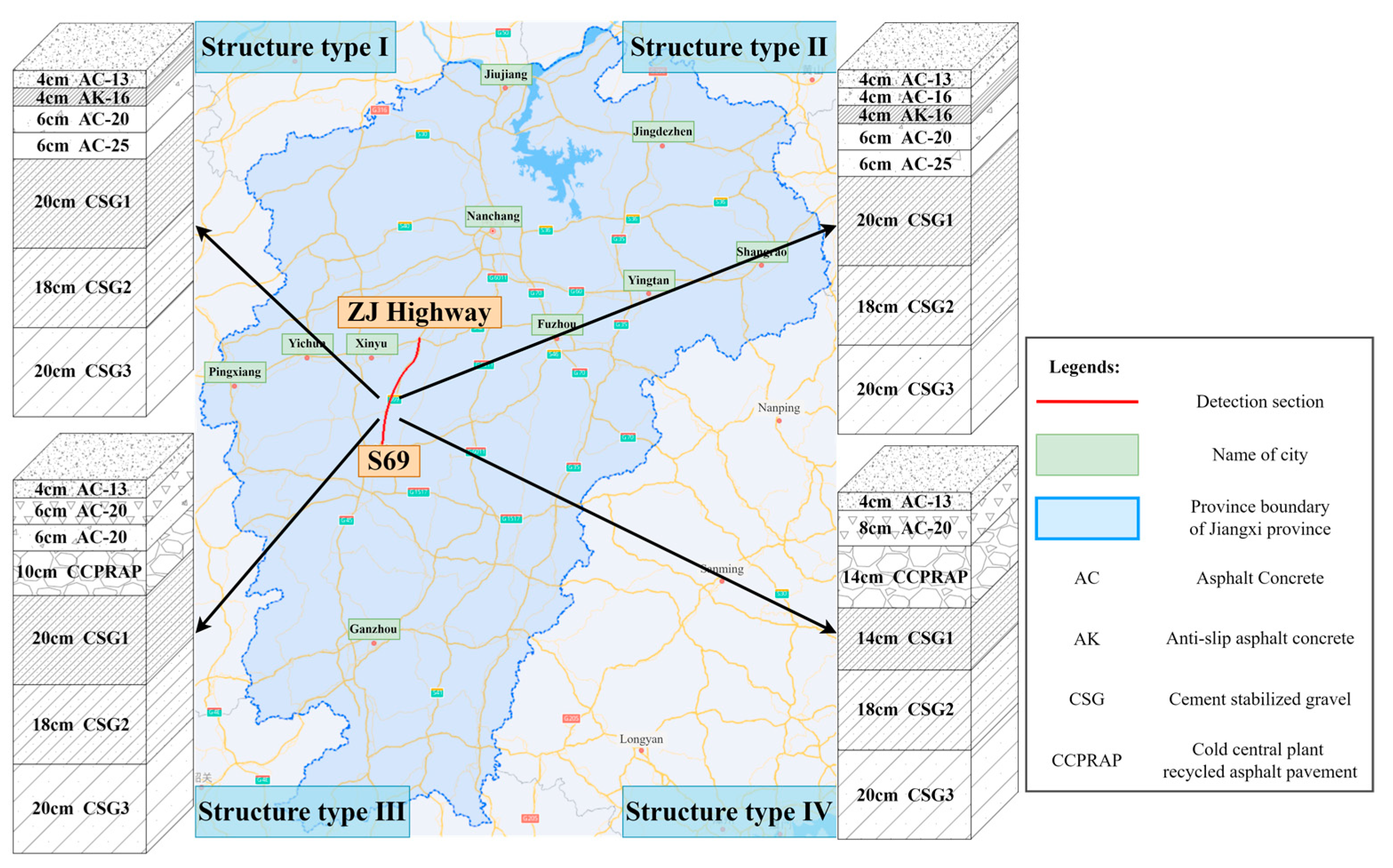
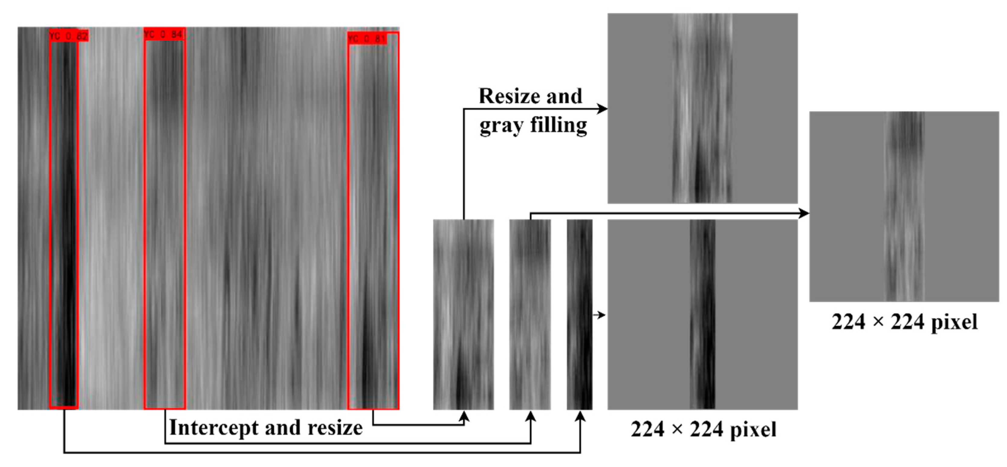
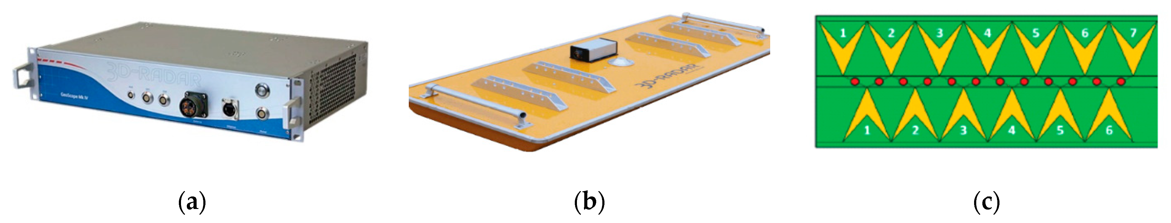
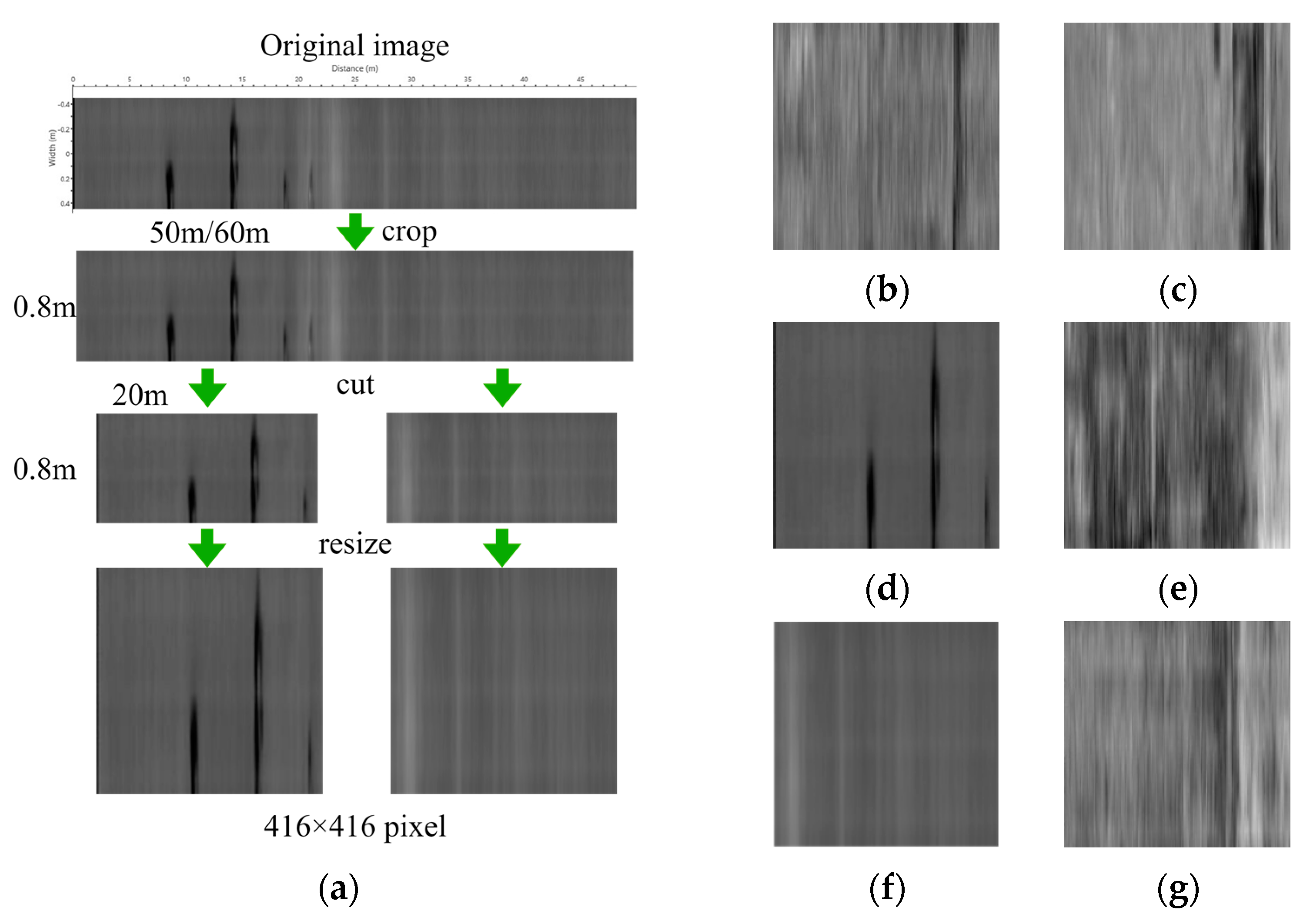
2.1. Acquisition and Pre-Processing GPR Images
2.2. Proposed Localization Model
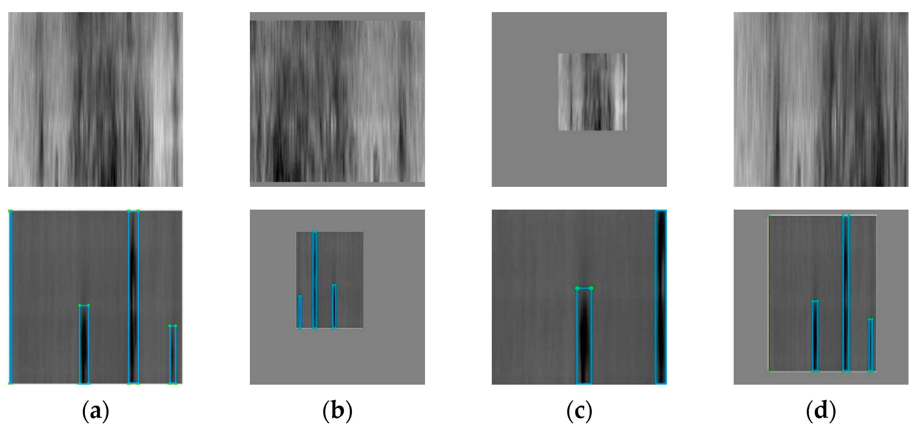
2.2.1. Distress Localization Dataset
- (1)
- Randomly crop an image;
- (2)
- Randomly resize an image in terms of its length and width;
- (3)
- Randomly distort the color gamut of an image.
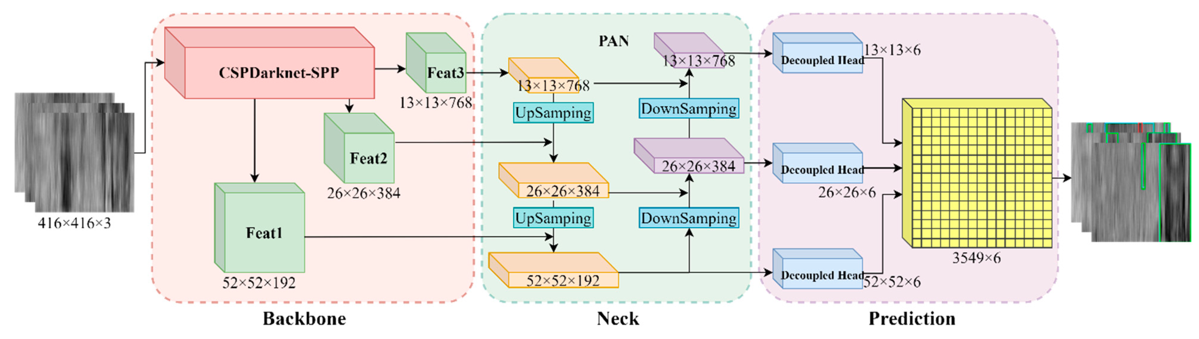
2.2.2. Structure of CP-YOLOX
- (1)
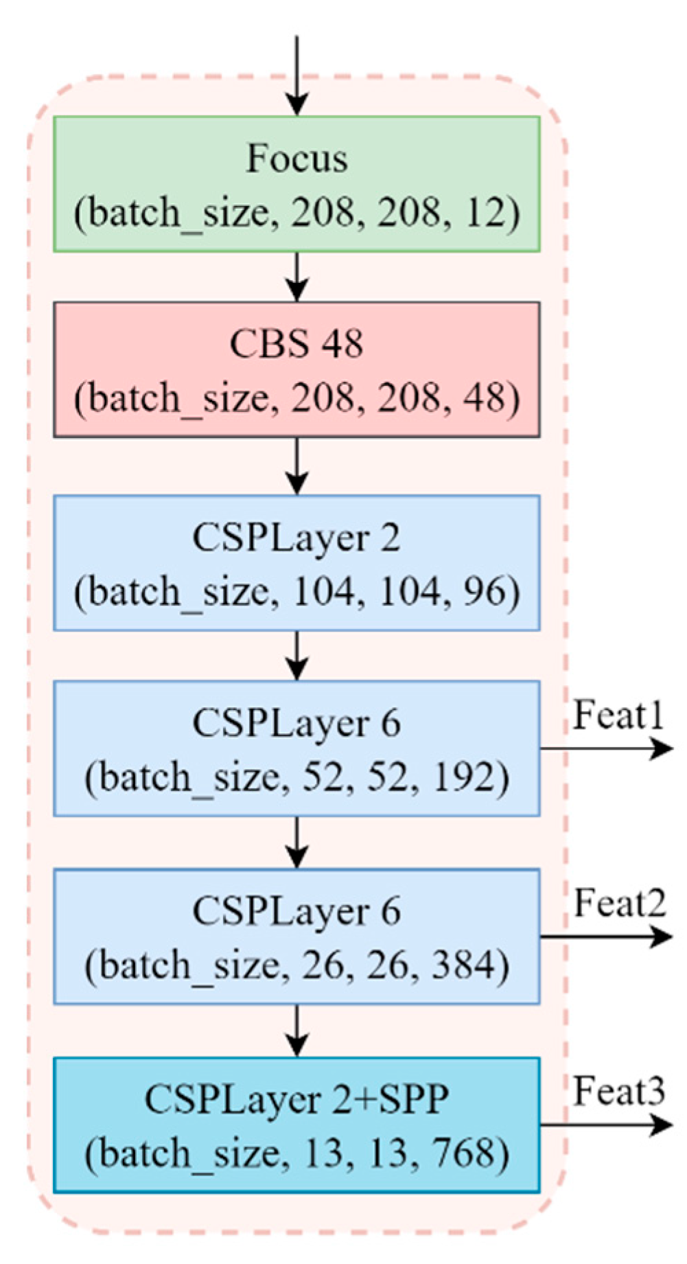
- Backbone
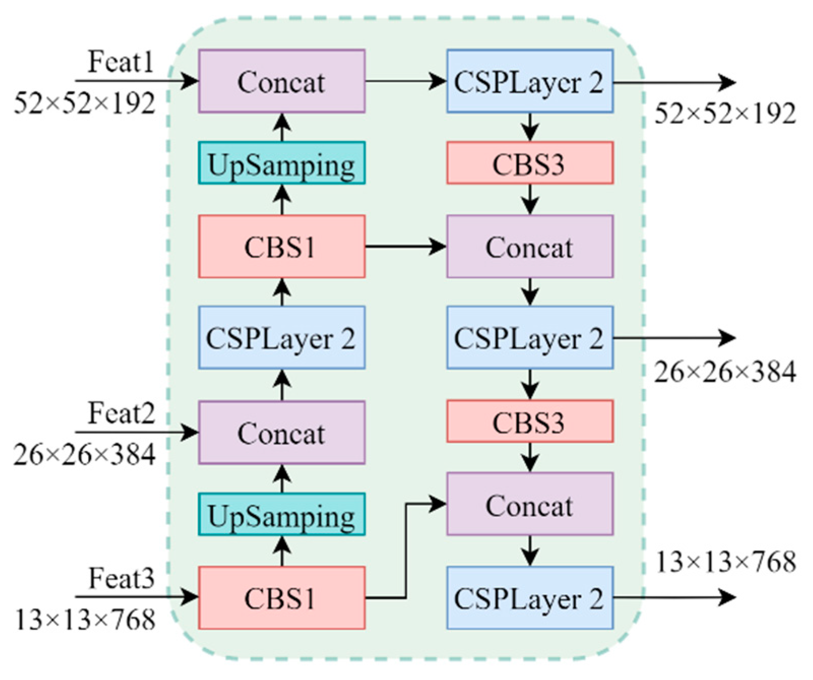
- (2)
- Neck
- (3)
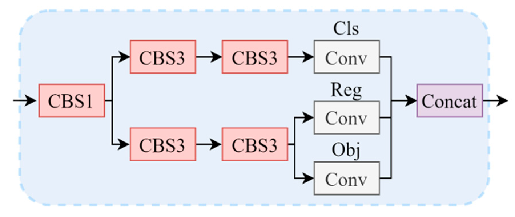
- Prediction
2.3. Proposed Classification Model
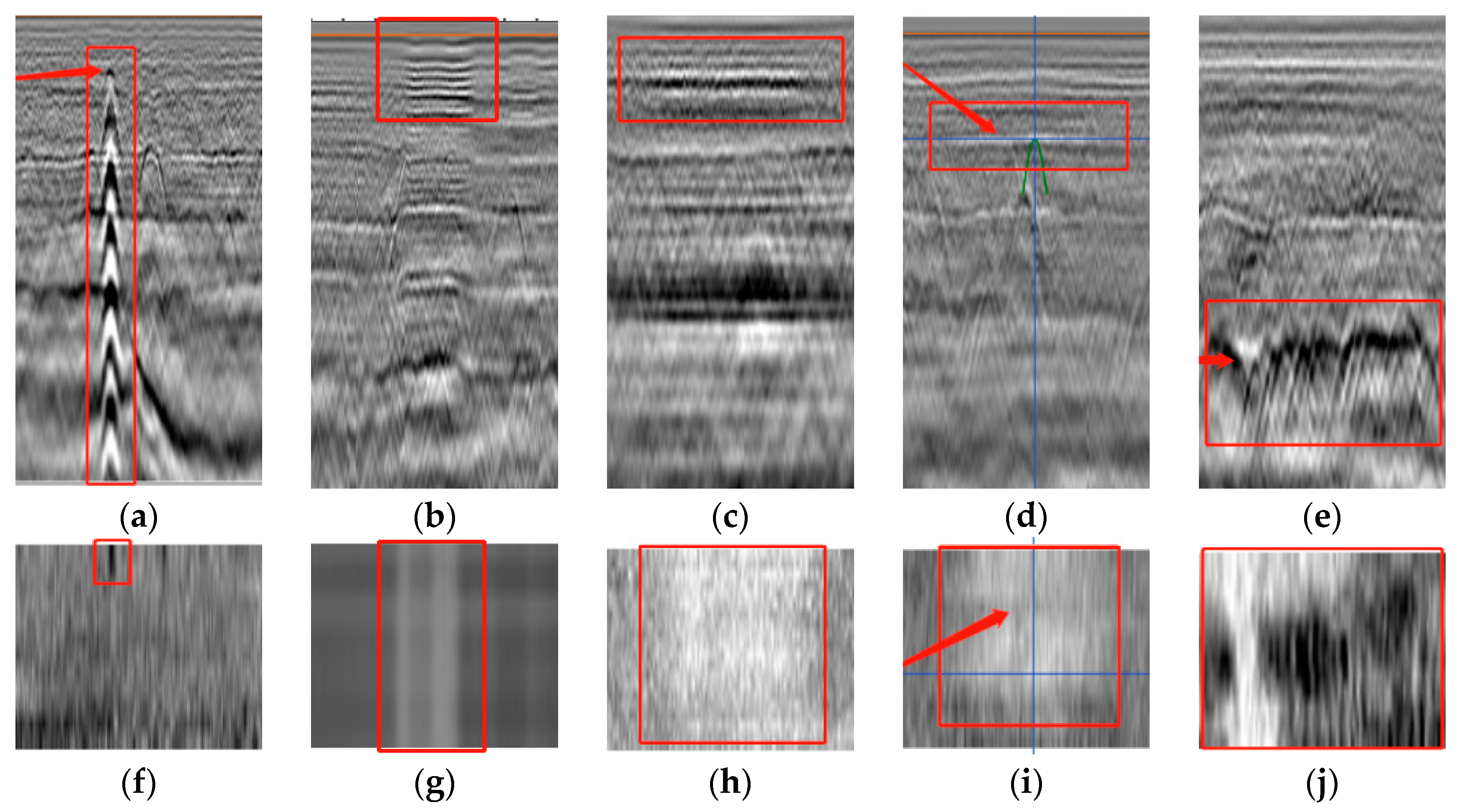
2.3.1. Distress Classification Dataset
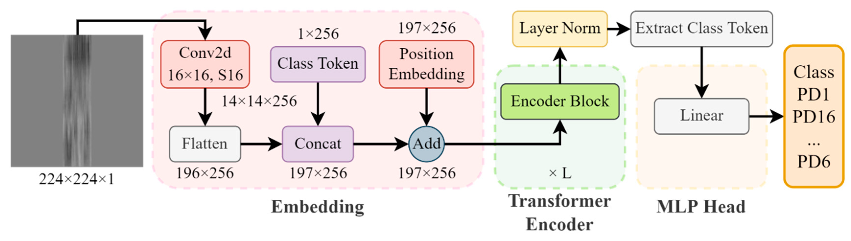
2.3.2. Structure of SViT
- (1)
- Embedding
- (2)
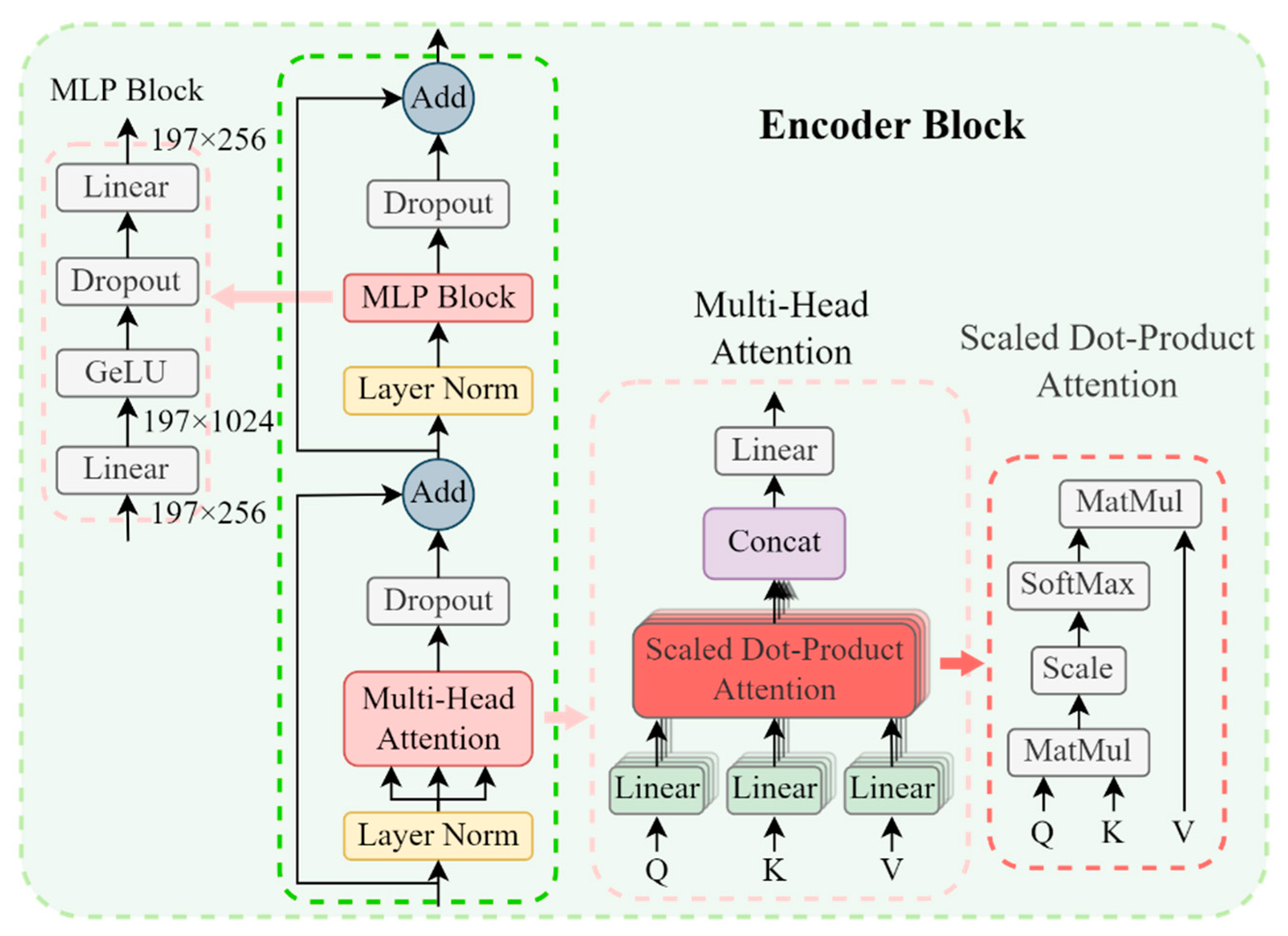
- Transformer Encoder
- (3)
- MLP Head
2.4. Learning Strategy
- (1)
- Overall
- (2)
- Training of CP-YOLOX
- (3)
- Training of SViT
3. Results and Discussion
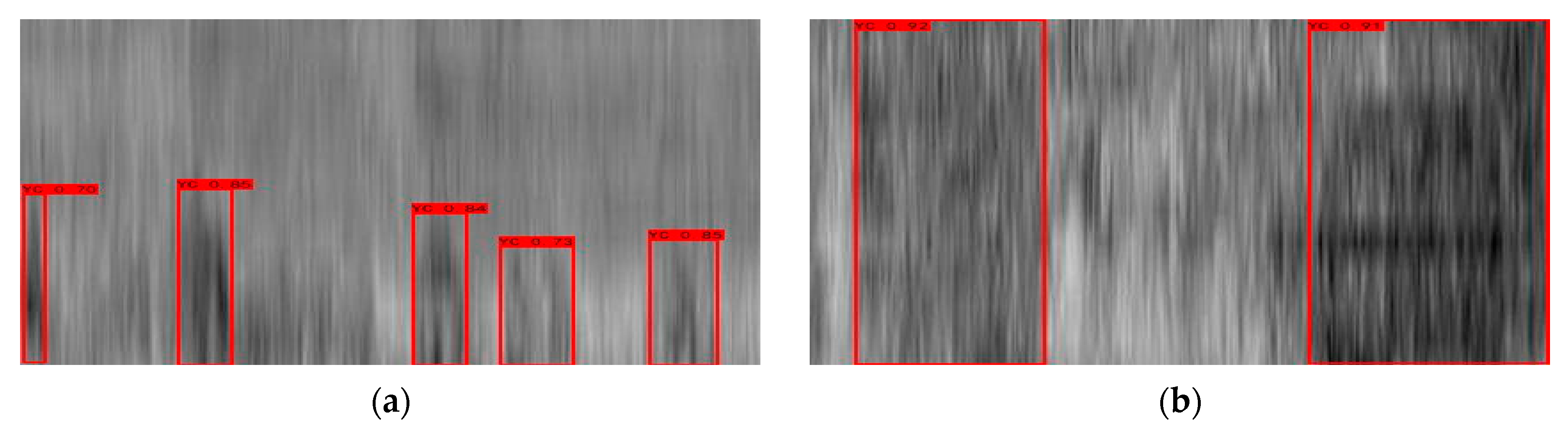
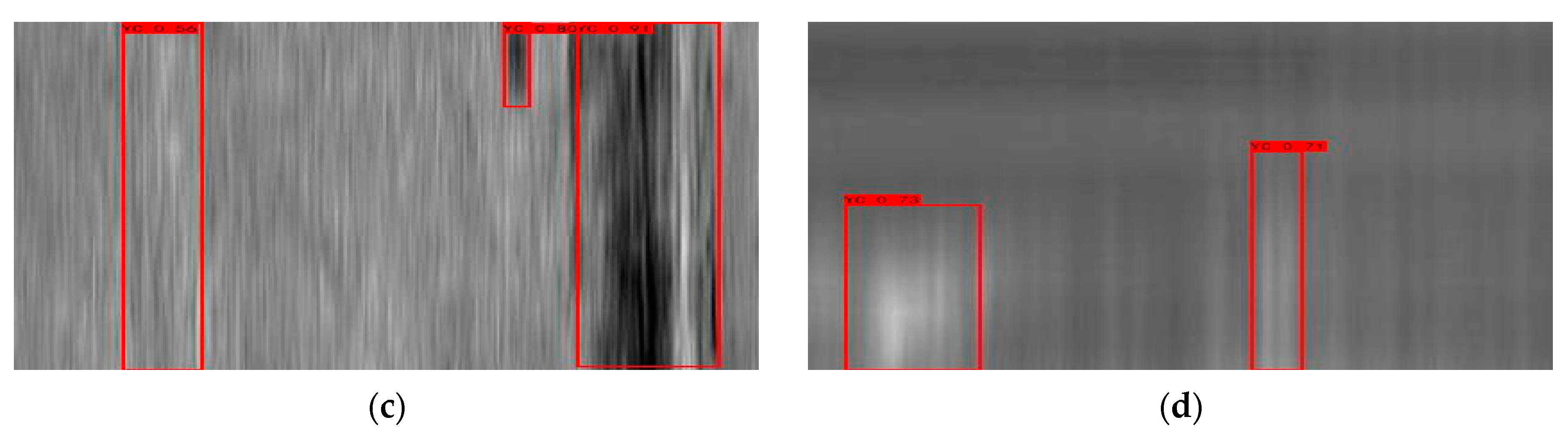
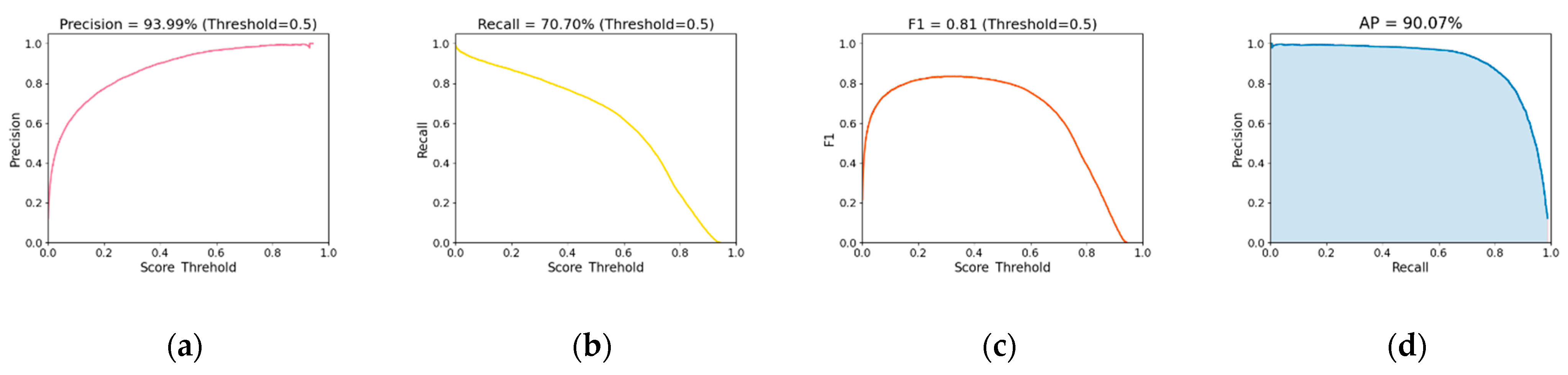
3.1. Analysis of Localization Results
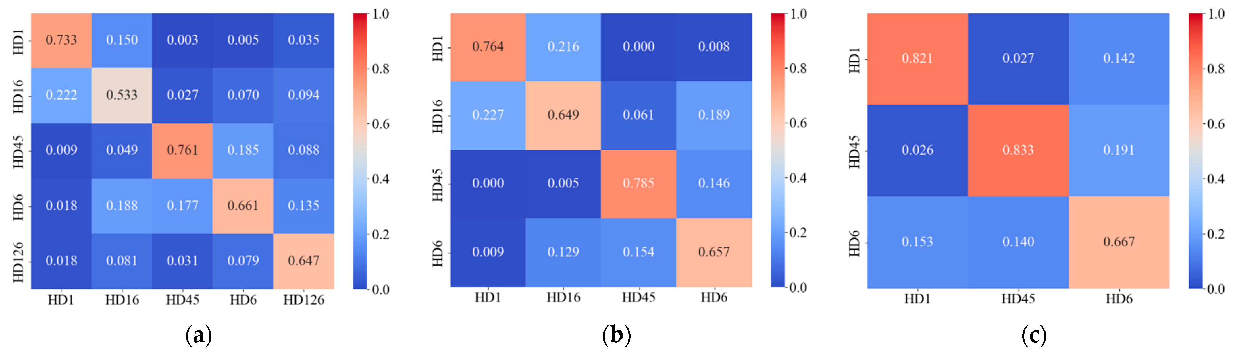
3.2. Analysis of Classification Results
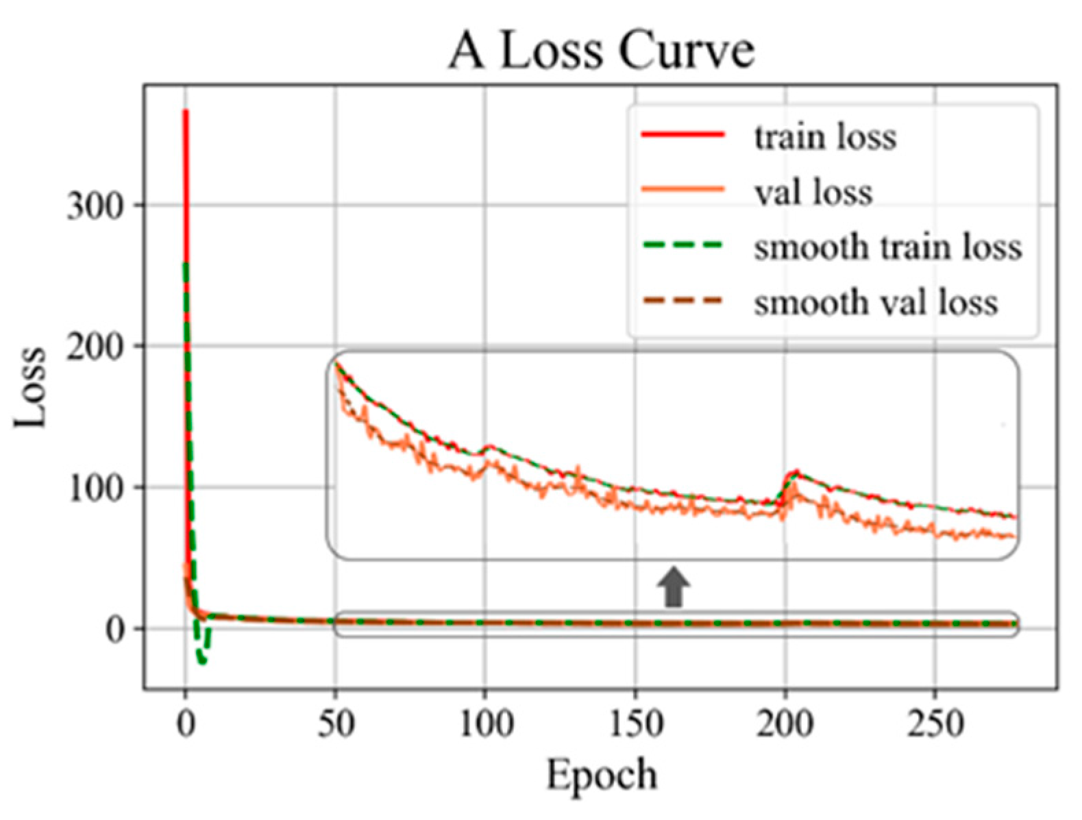
3.2.1. Results of Training and Testing
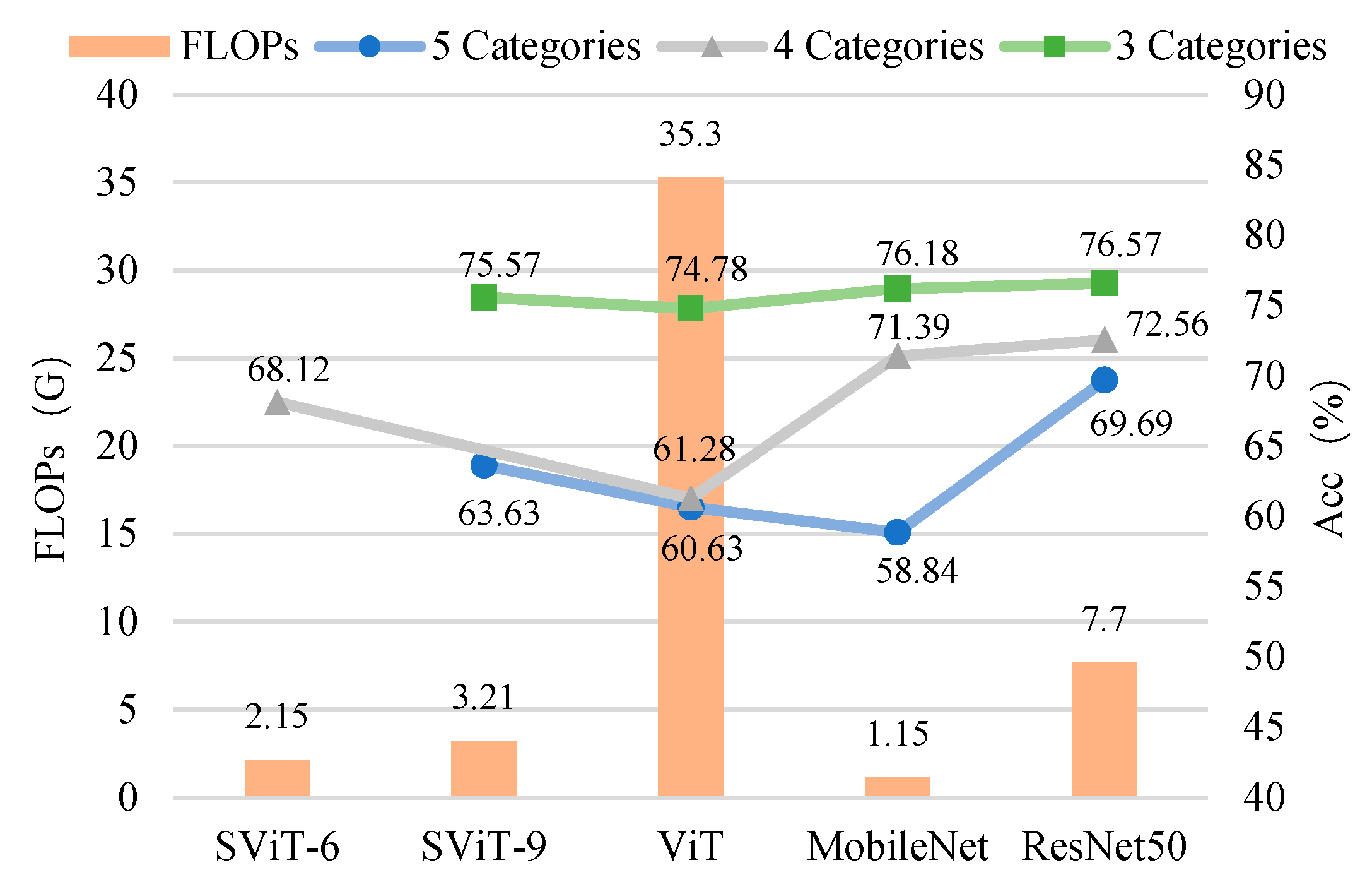
3.2.2. Prediction Results of Different Models
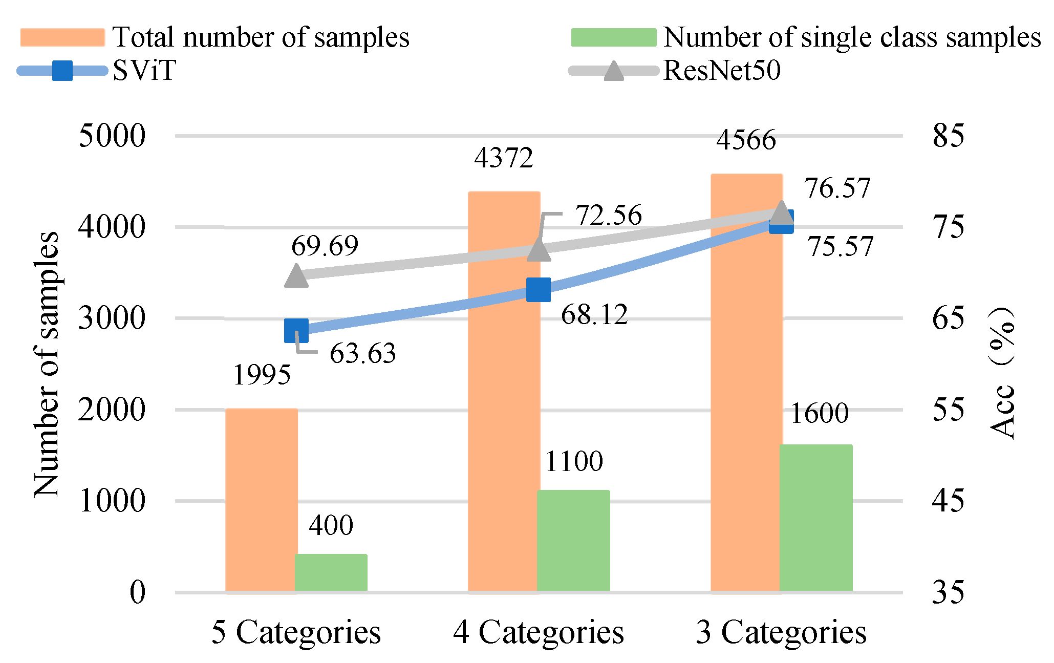
3.2.3. The Influence of Number of Samples on the Model
4. Conclusions
- (1)
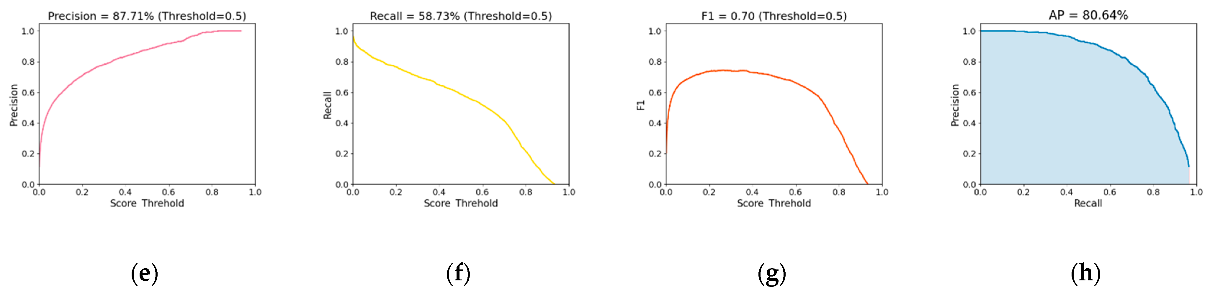
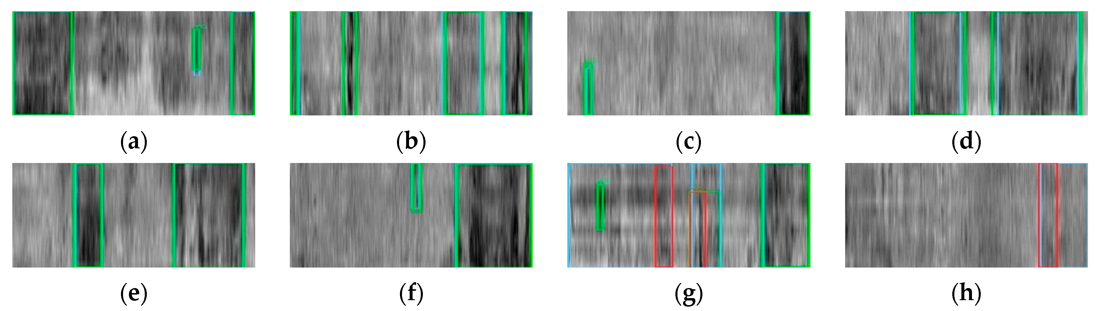
- The proposed CP-YOLOX model could localize anomalous waveforms caused by pavement distresses. With a confidence threshold of 0.5, the CP-YOLOX model localized anomalous waveforms with mAP of 80.64%, Precision of 87.71%, and Recall of 58.73%. The model processed radar images with a speed of 33.57 images/s.
- (2)
- The proposed SViT model was capable of detecting cracks, poor interlayer bonding, and mixture segregation distress in horizontal radar images. For the category without background noise, the model had a high prediction accuracy. Future studies should focus on how to suppress the noise waveform and on more detailed analysis of the disturbance waveform.
- (3)
- The proposed SViT model had fewer parameters and FLOPs, ensuring a high level of accuracy, which enables it to perform distress classification quickly. With the increase in GPR images, the gap between SViT and ResNet50 shrunk from 6.06% to 1%, indicating that more data samples had the potential to improve the performance of SViT. This demonstrated the superiority of the proposed model on the pavement distress classification.
- (4)
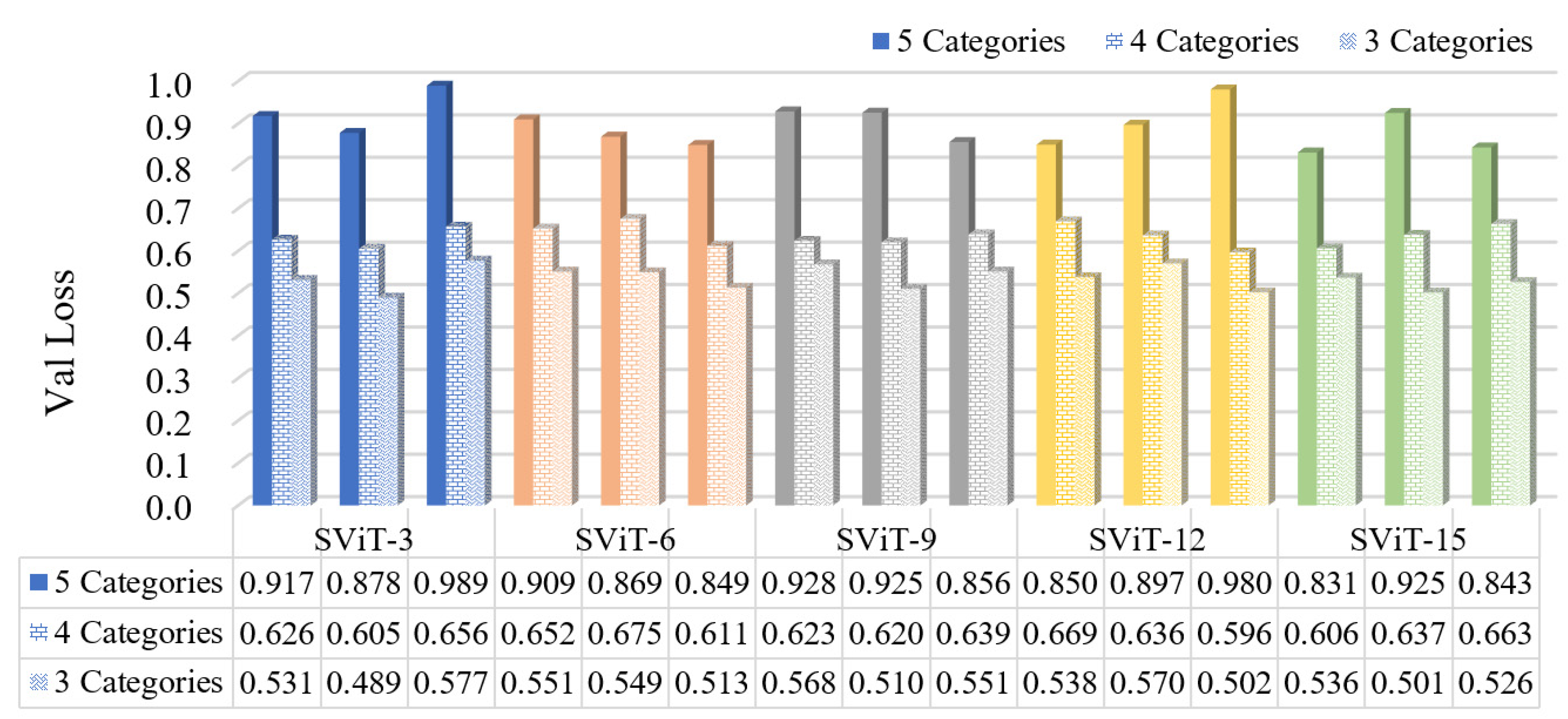
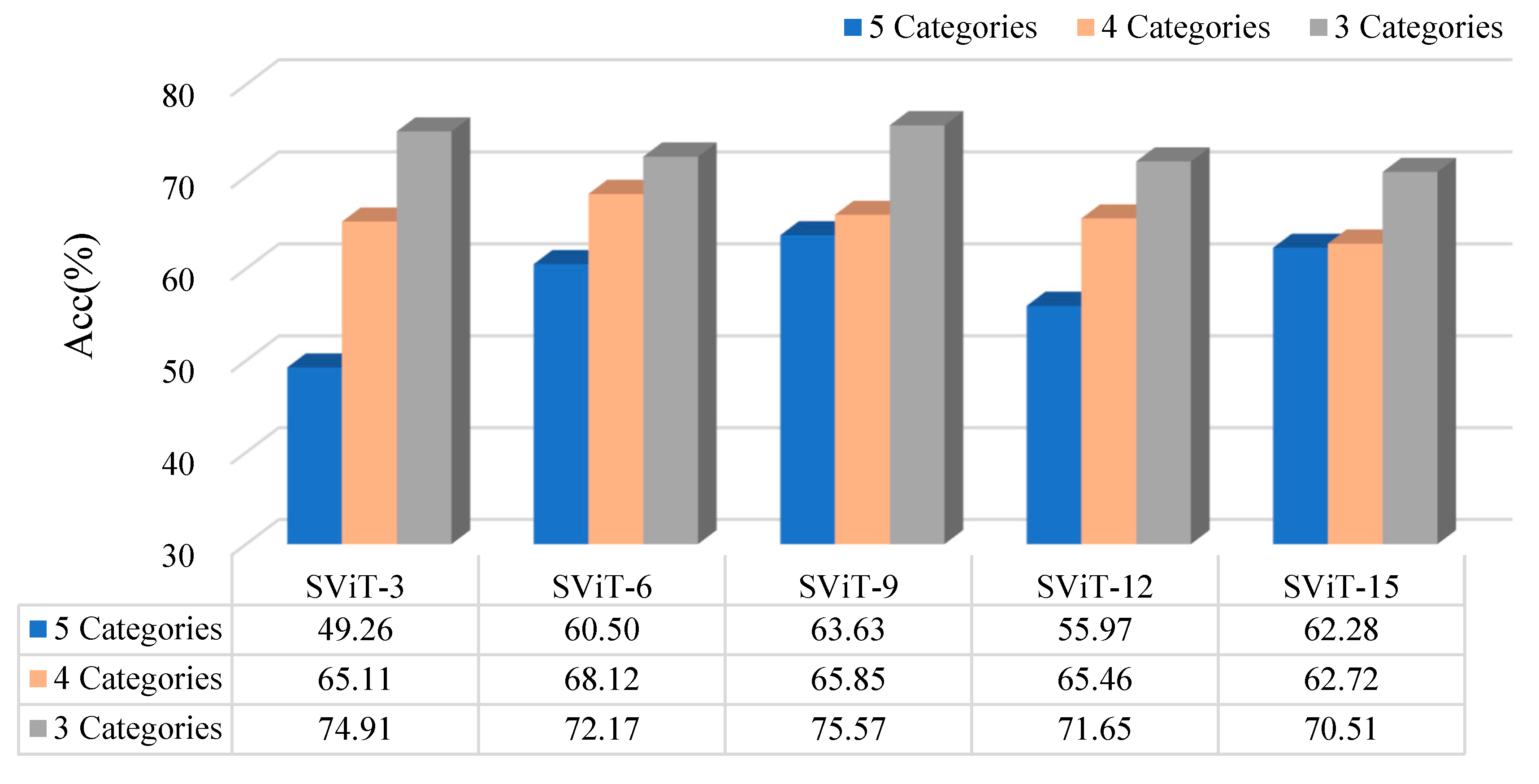
- In the three classification datasets, the 3-categories dataset had the highest accuracy, followed by the 4-categories dataset, and the 5-categories dataset had the lowest accuracy. However, the model trained based on the 5-categories dataset provided the most detailed basis for distress classification. Subsequently, we need to combine the horizontal detection results with the longitudinal radar images to determine the best classification method using 3D GPR.
Author Contributions
Funding
Institutional Review Board Statement
Informed Consent Statement
Data Availability Statement
Conflicts of Interest
Abbreviations
| Abbreviations | Full Name |
| 3D GPR | Three-dimensional ground penetrating radar |
| DL | Deep Learning |
| CNN | Convolutional Neural Network |
| ViT | Vision Transformer |
| SViT | Simplify Vision Transformers |
| YOLOX | You Only Look Once X |
| CP-YOLOX | CSP PAN YOLOX |
| CSP | Cross Stage Partial |
| SPP | Spatial Pyramid Pooling |
| CBS | Convolutional Batch normalization SiLU |
| PAN | Path Aggregation Network |
| SimOTA | Simplify Optimal Transport Assignment |
| HD | Horizontal Distress |
| MLP | Multi-Layer Perceptron |
| BP | Backward Propagation |
| mAP | mean average precision |
| NMS | Non-Max Suppression |
| FLOPs | floating-point operations |
References
- Benedetto, A.; Tosti, F.; Ciampoli, L.B.; D’Amico, F. An overview of ground-penetrating radar signal processing techniques for road inspections. Signal Process. 2017, 132, 201–209. [Google Scholar] [CrossRef]
- Zajícová, K.; Chuman, T. Application of ground penetrating radar methods in soil studies: A review. Geoderma 2019, 343, 116–129. [Google Scholar] [CrossRef]
- Tong, Z. Research on Pavement Distress Inspection Based on Deep Learning and Ground Penetrating Radar; Chang’an University: Xi’an, China, 2018; pp. 1–12. [Google Scholar]
- Cai, J.; Song, C.; Gong, X.; Zhang, J.; Pei, J.; Chen, Z. Gradation of limestone-aggregate-based porous asphalt concrete under dynamic crushing test: Composition, fragmentation and stability. Constr. Build. Mater. 2022, 323, 126532. [Google Scholar] [CrossRef]
- Klewe, T.; Strangfeld, C.; Kruschwitz, S. Review of moisture measurements in civil engineering with ground penetrating radar —Applied methods and signal features. Constr. Build. Mater. 2021, 278, 122250. [Google Scholar] [CrossRef]
- Luo, C.X. Research on the Application of Road Nondestructive Testing Technology Based on Three-Dimensional Ground Penetrating Radar; South China University of Technology: Guangzhou, China, 2018; pp. 55–69. [Google Scholar]
- Travassos, X.L.; Avila, S.L.; Ida, N. Artificial Neural Networks and Machine Learning techniques applied to Ground Penetrating Radar: A review. Appl. Comput. Inform. 2018, 17, 296–308. [Google Scholar] [CrossRef]
- Williams, R.M.; Ray, L.; Lever, J.H.; Burzynski, A.M. Crevasse Detection in Ice Sheets Using Ground Penetrating Radar and Machine Learning. IEEE J. Sel. Top. Appl. Earth Obs. Remote Sens. 2014, 7, 4836–4848. [Google Scholar] [CrossRef]
- Zhou, H.; Feng, X.; Zhang, Y.; Nilot, E.; Zhang, M.; Dong, Z.; Qi, J. Combination of Support Vector Machine and H-Alpha Decomposition for Subsurface Target Classification of GPR. In Proceedings of the 17th International Conference on Ground Penetrating Radar (GPR), Rapperswil, Switzerland, 18–21 June 2018; pp. 635–638. [Google Scholar]
- Kwon, H.; Kim, Y. BlindNet backdoor: Attack on deep neural network using blind watermark. Multimedia Tools Appl. 2022, 81, 6217–6234. [Google Scholar] [CrossRef]
- Kwon, H. MedicalGuard: U-Net Model Robust against Adversarially Perturbed Images. Secur. Commun. Netw. 2021, 2021, 1–8. [Google Scholar] [CrossRef]
- Kwon, H.; Yoon, H.; Choi, D. Data Correction For Enhancing Classification Accuracy By Unknown Deep Neural Network Classifiers. KSII Trans. Internet Inform. Syst. 2021, 15, 3243–3257. [Google Scholar] [CrossRef]
- Lecun, Y.; Bottou, L.; Bengio, Y.; Haffner, P. Gradient-based learning applied to document recognition. Proc. IEEE 1998, 86, 2278–2324. [Google Scholar] [CrossRef] [Green Version]
- LeCun, Y.; Bengio, Y.; Hinton, G. Deep learning. Nature 2015, 521, 436–444. [Google Scholar] [CrossRef]
- Vaswani, A.; Shazeer, N.; Parmar, N. Attention is all you need. In Proceedings of the 31st Conference on Neural Information Processing Systems (NIPS 2017), Long Beach, CA, USA, 4–9 December 2017. [Google Scholar]
- Dosovitskiy, A.; Beyer, L.; Kolesnikov, A. An image is worth 16x16 words: Transformers for image recognition at scale. arXiv 2020, arXiv:2010.11929. [Google Scholar]
- Tong, Z.; Gao, J.; Yuan, D. Advances of deep learning applications in ground-penetrating radar: A survey. Constr. Build. Mater. 2020, 258, 120371. [Google Scholar] [CrossRef]
- Liu, H.; Lin, C.; Cui, J.; Fan, L.; Xie, X.; Spencer, B.F. Detection and localization of rebar in concrete by deep learning using ground penetrating radar. Autom. Constr. 2020, 118, 103279. [Google Scholar] [CrossRef]
- Li, S.; Gu, X.; Xu, X.; Xu, D.; Zhang, T.; Liu, Z.; Dong, Q. Detection of concealed cracks from ground penetrating radar images based on deep learning algorithm. Constr. Build. Mater. 2020, 273, 121949. [Google Scholar] [CrossRef]
- Liu, Z.; Wu, W.; Gu, X.; Li, S.; Wang, L.; Zhang, T. Application of Combining YOLO Models and 3D GPR Images in Road Detection and Maintenance. Remote Sens. 2021, 13, 1081. [Google Scholar] [CrossRef]
- Sha, A.M.; Tong, Z.; Gao, J. Recognition and Measurement of Pavement Disasters Based on Convolutional Neural Networks. China J. Highway Trans. 2018, 31, 1–10. [Google Scholar]
- Hou, Y.; Chen, Y.H.; Gu, X.Y.; Mao, Q.; Cao, D.D. Automatic Identification of Pavement Objects and Cracks Using the Convolutional Auto-encoder. China J. Highway Transp. 2020, 33, 288–303. [Google Scholar]
- Yan, B.F.; Xu, Y.G.; Luan, J.; Lin, D.; Deng, L. Pavement Distress Detection Based on Faster R-CNN and Morphological Operations. China J. Highway Transp. 2021, 34, 181–193. [Google Scholar]
- Sha, A.M.; Cai, R.N.; Gao, J.; Tong, Z.; Li, S. Subgrade distresses recognition based on convolutional neural network. J. Chang’an Univ. (Nat. Sci. Ed.) 2019, 39, 1–9. [Google Scholar]
- Tong, Z.; Gao, J.; Zhang, H. Recognition, location, measurement, and 3D reconstruction of concealed cracks using convolutional neural networks. Constr. Build. Mater. 2017, 146, 775–787. [Google Scholar] [CrossRef]
- Gao, J.; Yuan, D.; Tong, Z.; Yang, J.; Yu, D. Autonomous pavement distress detection using ground penetrating radar and region-based deep learning. Measurement 2020, 164, 108077. [Google Scholar] [CrossRef]
- Tong, Z.; Yuan, D.; Gao, J.; Wei, Y.; Dou, H. Pavement-distress detection using ground-penetrating radar and network in networks. Constr. Build. Mater. 2019, 233, 117352. [Google Scholar] [CrossRef]
- Long, Z.J. Reverse-Time Migration Applied to Ground Penetrating Rader and Intelligent Recognition of Subsurface Targets; Xiamen University: Xiamen, China, 2018; pp. 1–4. [Google Scholar]
- Wang, H.; Ou, Y.S.; Liao, K.F.; Jin, L.N. GPR B-SCAN Image Hyperbola Detection Method Based on Deep Learning. Acta Electr. Sinica 2021, 49, 953–963. [Google Scholar]
- Kim, N.; Kim, S.; An, Y.-K.; Lee, J.-J. Triplanar Imaging of 3-D GPR Data for Deep-Learning-Based Underground Object Detection. IEEE J. Sel. Top. Appl. Earth Obs. Remote Sens. 2019, 12, 4446–4456. [Google Scholar] [CrossRef]
- Omwenga, M.M.; Wu, D.; Liang, Y.; Yang, L.; Huston, D.; Xia, T. Cognitive GPR for Subsurface Object Detection Based on Deep Reinforcement Learning. IEEE Internet Things J. 2021, 8, 11594–11606. [Google Scholar] [CrossRef]
- Ge, Z.; Liu, S.; Wang, F.; Li, Z.; Sun, J. Yolox: Exceeding yolo series in 2021. arXiv 2021, arXiv:2107.08430. [Google Scholar]
- Wang, C.Y.; Liao, H.Y.M.; Wu, Y.H.; Chen, P.Y.; Hsieh, J.W.; Yeh, I.H. CSPNet: A new backbone that can enhance learning capability of CNN. In Proceedings of the IEEE/CVF Conference on Computer Vision and Pattern Recognition Workshops, Seattle, WA, USA, 14–19 June 2020; pp. 390–391. [Google Scholar]
- Liu, S.; Qi, L.; Qin, H.; Shi, J.; Jia, J. Path aggregation network for instance segmentation. In Proceedings of the IEEE Conference on Computer Vision and Pattern Recognition, Salt Lake City, UT, USA, 18–23 June 2018; pp. 8759–8768. [Google Scholar]
- He, K.; Zhang, X.; Ren, S.; Sun, J. Spatial Pyramid Pooling in Deep Convolutional Networks for Visual Recognition. IEEE Trans. Pattern Anal. Mach. Intell. 2015, 37, 1904–1916. [Google Scholar] [CrossRef] [PubMed] [Green Version]
- Ioffe, S.; Szegedy, C. Batch normalization: Accelerating deep network training by reducing internal covariate shift. In Proceedings of the International Conference on Machine Learning, Lille, France, 6–11 July 2015; pp. 448–456. [Google Scholar]
- Ge, Z.; Liu, S.; Li, Z.; Yoshie, O.; Sun, J. Ota: Optimal transport assignment for object detection. In Proceedings of the IEEE/CVF Conference on Computer Vision and Pattern Recognition, Nashville, TN, USA, 20–25 June 2021; pp. 303–312. [Google Scholar]
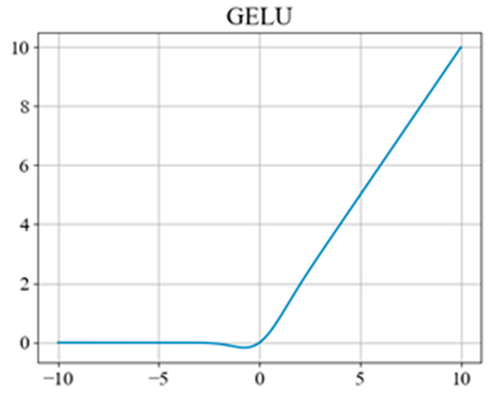
- Hendrycks, D.; Gimpel, K. Gaussian error linear units (gelus). arXiv 2016, arXiv:1606.08415. [Google Scholar]
- Zheng, Z.; Wang, P.; Liu, W.; Li, J.; Ye, R.; Ren, D. Distance-IoU loss: Faster and better learning for bounding box regression. In Proceedings of the AAAI Conference on Artificial Intelligence, New York, NY, USA, 7–12 February 2020; Volume 34, pp. 12993–13000. [Google Scholar]
- Kingma, D.P.; Ba, J. Adam: A method for stochastic optimization. arXiv 2014, arXiv:1412.6980. [Google Scholar]
- Li, Y.; Huang, H.; Xie, Q.; Yao, L.; Chen, Q. Research on a surface defect detection algorithm based on MobileNet-SSD. Appl. Sci. 2018, 8, 1678. [Google Scholar] [CrossRef] [Green Version]
- He, K.; Zhang, X.; Ren, S.; Sun, J. Deep residual learning for image recognition. In Proceedings of the IEEE Conference on Computer Vision and Pattern Recognition, Las Vegas, NV, USA, 27–30 June 2016; pp. 770–778. [Google Scholar]


| Type | Training and Validation Samples | Test Samples | ||
|---|---|---|---|---|
| Number of Objects | Number of Images | Number of Objects | Number of Images | |
| Anomalous waveform | 7453 | 3088 | 1592 | 600 |
| Layers | Kernel Size and Number | Input Size | Output Size | Stride | ||
|---|---|---|---|---|---|---|
| Focus | 3 × 4 = 12 | 416 × 416 | 208 × 208 | - | ||
| CBS3 | 3 × 3, 48 | 208 × 208 | 208 × 208 | 1 | ||
| CSPLayer 2 | CBS3 | 3 × 3, 96 | 208 × 208 | 104 × 104 | 2 | |
| CBS1 | 1 × 1, 48 | 1 × 1, 48 | 104 × 104 | 104 × 104 | 1 | |
| Res unit | - | 104 × 104 | 104 × 104 | 1 | ||
| CBS1 | 1 × 1, 96 | 104 × 104 | 104 × 104 | 1 | ||
| CSPLayer 6 | CBS3 | 3 × 3, 192 | 104 × 104 | 52 × 52 | 2 | |
| CBS1 | 1 × 1, 96 | 1 × 1, 96 | 52 × 52 | 52 × 52 | 1 | |
| Res unit | - | 52 × 52 | 52 × 52 | 1 | ||
| CBS1 | 1 × 1, 192 | 52 × 52 | 52 × 52 | 1 | ||
| CSPLayer 6 | CBS3 | 3 × 3, 384 | 52 × 52 | 26 × 26 | 2 | |
| CBS1 | 1 × 1, 192 | 1 × 1, 192 | 26 × 26 | 26 × 26 | 1 | |
| Res unit | - | 26 × 26 | 26 × 26 | 1 | ||
| CBS1 | 1 × 1, 384 | 26 × 26 | 26 × 26 | 1 | ||
| CSPLayer 2 + SPP | CBS3 | 3 × 3, 768 | 26 × 26 | 13 × 13 | 2 | |
| SPP | 1 × 1, 384 1 × 1, 5 × 5, 9 × 9, 13 × 13, 384 1 × 1, 768 | 13 × 13 | 13 × 13 | 1 | ||
| CBS1 | 1 × 1, 384 | 1 × 1, 384 | 13 × 13 | 13 × 13 | 1 | |
| Res unit | - | 13 × 13 | 13 × 13 | 1 | ||
| CBS1 | 1 × 1, 768 | 13 × 13 | 13 × 13 | 1 | ||
| Layers | Kernel Size | Channel | Input Size | Output Size | Stride |
|---|---|---|---|---|---|
| CBS1 | 1 × 1 | 384 | 13 × 13 | 13 × 13 | 1 |
| UpSamping | - | 384 | 13 × 13 | 26 × 26 | - |
| Concat | - | 768 | 26 × 26 | 26 × 26 | - |
| CSPLayer 2 | (1 × 1, 3 × 3) × 2 | 384 | 26 × 26 | 26 × 26 | 1 |
| CBS1 | 1 × 1 | 192 | 26 × 26 | 26 × 26 | 1 |
| UpSamping | - | 192 | 26 × 26 | 52 × 52 | - |
| Concat | - | 384 | 52 × 52 | 52 × 52 | - |
| CSPLayer 2 | (1 × 1, 3 × 3) × 2 | 192 | 52 × 52 | 52 × 52 | 1 |
| CBS3 | 3 × 3 | 192 | 52 × 52 | 26 × 26 | 2 |
| Concat | - | 384 | 26 × 26 | 26 × 26 | - |
| CSPLayer 2 | (1 × 1, 3 × 3) ×2 | 384 | 26 × 26 | 26 × 26 | 1 |
| CBS3 | 3 × 3 | 384 | 26 × 26 | 13 × 13 | 2 |
| Concat | - | 768 | 13 × 13 | 13 × 13 | - |
| CSPLayer 2 | (1 × 1, 3 × 3) ×2 | 768 | 13 × 13 | 13 × 13 | 1 |
| Classification Method | Category | Category Number | ||||
|---|---|---|---|---|---|---|
| 1 | HD1 | HD16 | HD45 | HD6 | HD126 | 5 |
| 2 | HD1 | HD16 | HD45 | HD6 | 4 | |
| 3 | HD1 | HD45 | HD6 | 3 | ||
| Category | HD1 | HD16 | HD45 | HD6 | HD126 | |
|---|---|---|---|---|---|---|
| 5 Categories |  |  |  |  |  | |
| Training | Samples | 1072 | 2172 | 1366 | 2448 | 395 |
| Data set | 400 | 400 | 400 | 400 | 395 | |
| Testing | Data set | 178 | 467 | 120 | 748 | 79 |
| Category | HD1 | HD16 | HD45 | HD6 | ||
| 4 Categories |  |  |  |  | ||
| Training | Samples | 1072 | 2172 | 1366 | 2843 | |
| Data set | 1072 | 1100 | 1100 | 1100 | ||
| Testing | Data set | 178 | 467 | 120 | 827 | |
| Category | HD1 | HD45 | HD6 | |||
| 3 Categories |  | 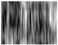 | 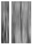 | |||
| Training | Samples | 3244 | 1366 | 2843 | ||
| Data set | 1600 | 1366 | 1600 | |||
| Testing | Data set | 645 | 120 | 827 | ||
| Model | Patch Pixel | Layer | Hidden Size | MLP Size | Heads | Params | FLOPs |
|---|---|---|---|---|---|---|---|
| SViT-3 | 16 × 16 | 3 | 256 | 1024 | 4 | 2.49 M | 1.09 G |
| SViT-6 | 16 × 16 | 6 | 256 | 1024 | 4 | 4.86 M | 2.15 G |
| SViT-9 | 16 × 16 | 9 | 256 | 1024 | 4 | 7.23 M | 3.21 G |
| SViT-12 | 16 × 16 | 12 | 256 | 1024 | 4 | 9.6 M | 4.27 G |
| SViT-15 | 16 × 16 | 15 | 256 | 1024 | 4 | 11.96 M | 5.33 G |
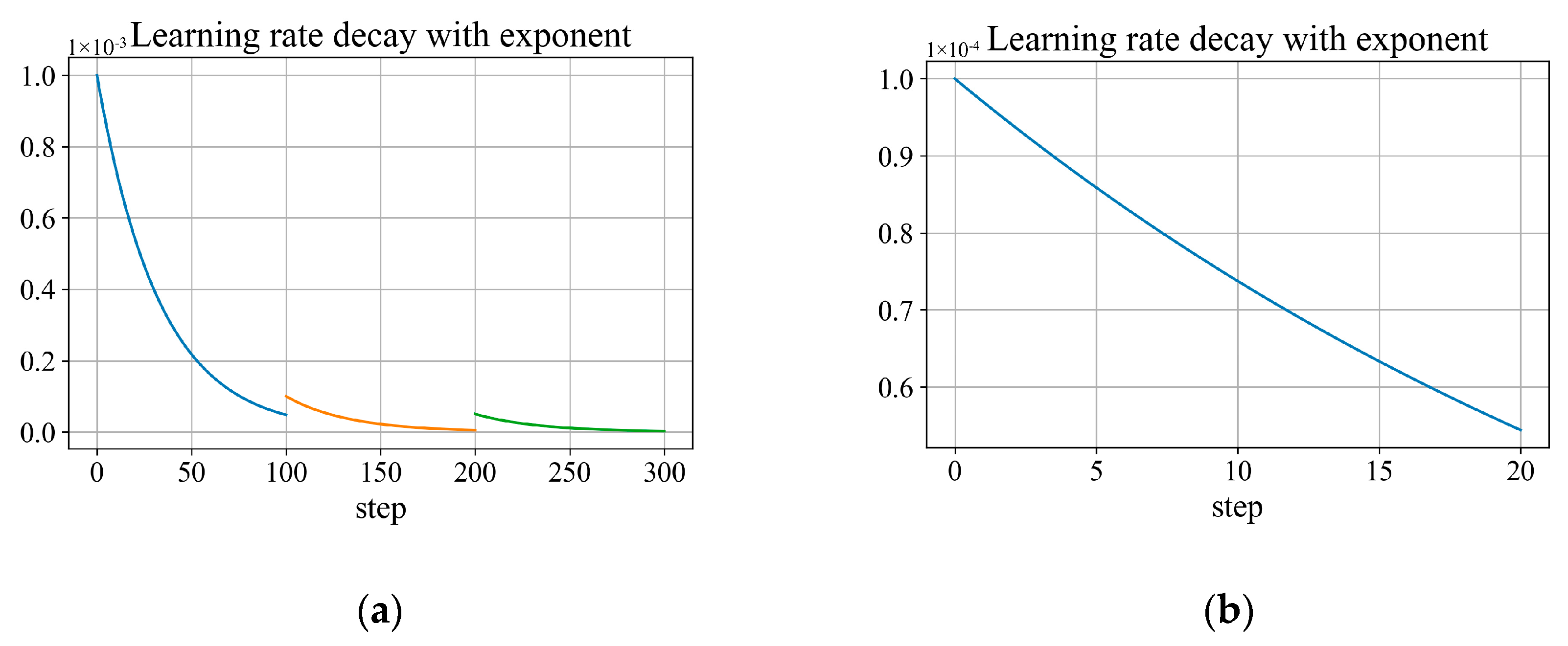
| Model | Learning Rate Decay Coefficient | Batch Size | Epoch | Base Learning Rate | Optimizer |
|---|---|---|---|---|---|
| CP-YOLOX | γ = 0.97 | 16 | 100 | 1 × 10⁻³ | Adam |
| 100 | 1 × 10⁻⁴ | ||||
| 100 | 5 × 10⁻⁵ | ||||
| SViT | γ = 0.97 | 32 | 20 | 1 × 10⁻⁴ | Adam |
| Model | Size (Pixels) | Precision (%) | Recall (%) | F1 Score | mAP (%) | FPS (Images/s) | Inference Time (ms) |
|---|---|---|---|---|---|---|---|
| CP-YOLOX | 416 × 416 | 87.71 | 58.73 | 0.70 | 80.64 | 33.57 | 29.8 |
| Model | 5 Categories Dataset | 4 Categories Dataset | 3 Categories Dataset |
|---|---|---|---|
| SViT-3 | 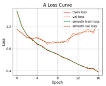 |  | 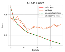 |
| SViT-6 |  |  |  |
| SViT-9 |  |  |  |
| SViT-12 |  |  |  |
| SViT-15 |  |  |  |
| Model | Acc (%) | Params | FLOPs | ||
|---|---|---|---|---|---|
| 5 Categories | 4 Categories | 3 Categories | |||
| SViT-6 | — | 68.12 | — | 4.86 M | 2.15 G |
| SViT-9 | 63.63 | — | 75.57 | 7.23 M | 3.21 G |
| ViT | 60.63 | 61.28 | 74.78 | 85.8 M | 35.3 G |
| MobileNet | 58.84 | 71.39 | 76.18 | 3.23 M | 1.15 G |
| ResNet50 | 69.69 | 72.56 | 76.57 | 23.6 M | 7.7 G |
Publisher’s Note: MDPI stays neutral with regard to jurisdictional claims in published maps and institutional affiliations. |
© 2022 by the authors. Licensee MDPI, Basel, Switzerland. This article is an open access article distributed under the terms and conditions of the Creative Commons Attribution (CC BY) license (https://creativecommons.org/licenses/by/4.0/).
Share and Cite
Yang, J.; Ruan, K.; Gao, J.; Yang, S.; Zhang, L. Pavement Distress Detection Using Three-Dimension Ground Penetrating Radar and Deep Learning. Appl. Sci. 2022, 12, 5738. https://doi.org/10.3390/app12115738
Yang J, Ruan K, Gao J, Yang S, Zhang L. Pavement Distress Detection Using Three-Dimension Ground Penetrating Radar and Deep Learning. Applied Sciences. 2022; 12(11):5738. https://doi.org/10.3390/app12115738
Chicago/Turabian StyleYang, Jiangang, Kaiguo Ruan, Jie Gao, Shenggang Yang, and Lichao Zhang. 2022. "Pavement Distress Detection Using Three-Dimension Ground Penetrating Radar and Deep Learning" Applied Sciences 12, no. 11: 5738. https://doi.org/10.3390/app12115738
APA StyleYang, J., Ruan, K., Gao, J., Yang, S., & Zhang, L. (2022). Pavement Distress Detection Using Three-Dimension Ground Penetrating Radar and Deep Learning. Applied Sciences, 12(11), 5738. https://doi.org/10.3390/app12115738