Development of a Multilayer Perceptron Neural Network for Optimal Predictive Modeling in Urban Microcellular Radio Environments

Abstract

Modern cellular communication networks are already being perturbed by large and steadily increasing mobile subscribers in high demand for better service quality. To constantly and reliably deploy and optimally manage such mobile cellular networks, the radio signal attenuation loss between the path lengths of a base transmitter and the mobile station receiver must be appropriately estimated. Although many log-distance-based linear models for path loss prediction in wireless cellular networks exist, radio frequency planning requires advanced non-linear models for more accurate predictive path loss estimation, particularly for complex microcellular environments. The precision of the conventional models on path loss prediction has been reported in several works, generally ranging from 8–12 dB in terms of Root Mean Square Error (RMSE), which is too high compared to the acceptable error limit between 0 and 6 dB. Toward this end, the need for near-precise machine learning-based path loss prediction models becomes imperative. This work develops a distinctive multi-layer perception (MLP) neural network-based path loss model with well-structured implementation network architecture, empowered with the grid search-based hyperparameter tuning method. The proposed model is designed for optimal path loss approximation between mobile station and base station. The hyperparameters examined include the neuron number, learning rate and hidden layers number. In detail, the developed MLP model prediction accuracy level using different learning and training algorithms with the tuned best values of the hyperparameters have been applied for extensive path loss experimental datasets. The experimental path loss data is acquired via a field drive test conducted over an operational 4G LTE network in an urban microcellular environment. The results were assessed using several first-order statistical performance indicators. The results show that prediction errors of the proposed MLP model compared favourably with measured data and were better than those obtained using conventional log-distance-based path loss models.

1. Introduction

Path loss models are unique prediction models employed by telecom network engineers to estimate the signal coverage area being served by a given transmitter during networking and management [1,2,3]. However, developing these signal path loss models with the optimal accuracy it deserves is a complex and significant problem in the planning of telecommunication networks. The conventional log-distance-based statistical models available in the literature, such as the cluster factor model, COST 234 Hata Model, free space model, Hata model and Lee models, lack accuracy for realistic path loss prediction applications in cellular mobile networks environments [4,5,6,7,8,9,10,11]. The aforementioned fundamental limitation of the conventional models is usually very pronounced when the respective models have been applied in cellular radio environments other than the developed and designed environment [12,13]. This scenario is mainly due to dissimilarities and variations in environmental formations (hilly, mountainous or quasi-plain), weather conditions, soil electrical properties and terrain type (open, rural, suburban or urban) that exist in different radio propagation locations, cities and countries [14,15,16,17,18,19,20,21,22,23]. For example, the Hata loss model was developed based on extensive practical measurements carried out in Japan at transmission frequency ranges of 150 to 1920 MHz and macrocellular communication distances of 1 to 100 km, with the mobile station and base station antenna heights of 2 to 3 and 30 to 1000 m, respectively [24]. This model, including other aforementioned conventional ones, is also generally limited in capturing the non-linear relationship between the independent variable (e.g., path loss) and dependent variable (e.g., distance) [25]. The precision of these conventional models on path loss prediction has been reported in many previous works to generally range from 8–12 dB in terms of Root Mean Square Error (RMSE), which is exceptionally higher than the acceptable values [9,14,15].

Recently, an Artificial Neural Network (ANN), a unique artificial intelligence soft computing and modelling technique, has been acknowledged and proven to solve function approximation and pattern classification problems [26]. Some ANN models exist in the literature; the key ones are Radial Basis Function models, Multilayer Perception Models, Generalized Neural Network models, etc. Among these models, the MLP ANN models have stood out most recently because they are very robust and popular for learning, function approximation, and pattern classification [27,28,29,30]. The MLP ANN possess many robust algorithms that can be explored to carry out more proficient adaptive nonlinear statistical modelling over the classical logistic regression methods [14,15,16,17,18,19,20,21,22,23] that are frequently engaged in developing predictive models. This robustness can be ascribed to their acknowledged special ability to learn, predict, and classify non-linear data using experience and preceding samples introduced to the network model. Huang [31] also noted that the MLP is characteristically good for input-output data mapping. Generally, a clear-cut underlining capability of ANN-based models over the conventional log-distance-based models is their large degrees of freedom structure which provides means for fitting many datasets with non-linear or linear correlation patterns. The concept of intelligent-based ANN models for optimal and adaptive prognostic estimations of path losses was introduced to surmount the limitations of existing empirically and deterministically developed log-distance models [32,33]. In the paper, the availability of manifold resourceful training algorithms and hypermeters of MLP ANN that can be tuned to further boost its extrapolative data analysis is worth exploring in this paper for optimal predictive modelling. Hence, the “Development of a Multilayer Perception Neural Network for Optimal Predictive Modeling in Urban Microcellular Radio Environments is self-evident.” Other key robust advantages of the general ANNs are highlighted in Section 2.3.

Though several ANN models exist in the literature, a critical, challenging task remains in developing and using them appropriately through the correct selection of its network structural design with the required input elements and hyperparameters to solve peculiar predictive mapping and functional problems. The quest to address this issue is the leading motivation for this research paper. However, one primary challenge in using the MLP model is correctly selecting its network architecture with the required input elements (hyperparameters) to solve a particular mapping problem [34]. Another critical challenge with neural network models is the problem of determining the input data variables that must correlate with the target variables [35,36].

This paper develops a distinctive MLP-based path loss model with well-structured implementation network architecture, empowered with the grid search-based hyperparameter tuning method for optimal path loss approximation between mobile-station and base-station path lengths. The hyperparameters include the neuron number, learning rate and hidden layers number. In detail, the developed MLP model prediction accuracy level using different learning and training algorithms with the tuned best values of the hyperparameters have been applied for extensive path loss experimental datasets. The datasets were acquired via field drive tests conducted in Long Term Evolution (LTE) in urban microcellular radio networks. For the development and implementation of the MLP-ANNs model, we utilized version 2018a of the MATLAB neural networks toolbox. The toolbox provides the required user interface, algorithm and platform to train, test, validate, visualize and simulate networks with the desired number of layers, neurons and activation functions.

In particular, the contributions of this paper are summarized as follows:

• ▪ A distinctive MLP neural network-based path loss model with well-structured implementation network architecture, embedded with the precise transfer function, neuron number, learning algorithm and hidden layers, is developed for optimal path loss approximation between mobile-station and base-station path lengths.
• ▪ The developed MLP neural network model was tested and validated for realistic path loss prediction using extensive experimental signal attenuation loss datasets acquired via field drive test conducted over LTE networks in urban microcellular radio environments and tested using first-order statistical performance indicators.
• ▪ Optimization of the projected model via hyperparameter tuning leveraging the grid search algorithm analyses of the experimental path loss data.
• ▪ Optimal prediction efficacy of the developed MLP neural network model compared with well-structured implementation architecture over standard log-distance models using several first-order statistical performance indicators.

The remainder of this work is structured in the following manner. Section 2 outlines the background information, such as radio propagation mechanisms, log-distance-based path loss prediction models, and the basis of artificial neural networks (ANN). Section 3 presents the methodology detailing the neural network implementation for predictive modelling. Section 4 provides the results, analysis, evaluation of the introduced neural network model at different study locations, comparison of the developed neural network model with log-distance models, and discussions. Finally, the conclusion is given in Section 5.

2. Theoretical Background

The theoretical background covers the radio propagation mechanism, log-distance-based path loss prediction models and artificial neural network systems.

2.1. Radio Propagation Mechanism

When radio signals travel, which are a form of electromagnetic waves, they interact with the media and objects they travel through. In the sequence of their interaction, the radio signals become weaker owing to refraction, reflection, diffraction, absorption and other propagation phenomena. The resultant effect of all the phenomena on propagated signals is signal propagation loss. The characteristics of the pathway or medium through which the radio signals travel determine the amount of propagation loss and the quality of the received signal that is attainable at the receiving terminal. Radio propagation loss is also governed by other sundry elements, particularly the transmitter power, receiver sensitivity and general antenna parameters such as antenna gain, antenna height and receiver location [1,2,37,38].

The prominent factors that influence the number of signal path losses in a medium include diffraction, reflection, refraction, scattering and absorption, to mention a few. For example, diffraction arises when radio waves collide with huge obstacles compared to the propagating signal wavelengths. Moreover, diffraction occurs when radio signals bend around objects, especially those with sharp edges. This alteration often empowers the received radio signal energy to spread around the boundaries of the obstructing object [39,40]. Diffraction is also influenced by the phase, amplitude, pathway and frequency of the transmitted waves.

The environment in which the radio frequency signals travel (or are propagated) will undoubtedly negatively impact the signal. For example, radio wave signals and propagation loss vary extensively in correspondence to the terrain landscape, building structures and population density. Marshy, damp and sandy terrain also attenuate radio signals, primarily propagated low-frequency signals. In other words, signals travel faster over conducive terrain than in sandy and marshy or damp terrains.

2.2. Log-Distance-Based Path Loss Prediction Models

Generally, path loss models are a set of mathematical models, expressions, resources and algorithms used for signal attenuation loss prediction between the paths of a base transmitter and the mobile station receiver. These models are helpful planning tools that assist the radio network designers of cellular telecommunication systems in optimally positioning base station transmitters to meet the desired signal coverage level and service quality requirements of the networks.

The predictive performance of any path loss model is determined by the resultant prediction accuracy with actual field measured loss data.

The log-distance-based path loss models are models whose average power loss logarithmically depends on distance (transmission path length) intertwined with a propagation exponent modelling parameter. The propagation exponent is usually employed to account for a specific radio propagation environment. They can also be described as simplified models that attempt to model variations, fluctuations and attenuations in the received signal power. Examples of log-distance-based models include the Walficsh–Ikegami, Walficsh Bertoni, cluster factor, COST 234 Hata, Hata Okumura, SUI model, Lee model, Egli Model and others [41]. Though these models have varying frequency validity thresholds, different correction factors have been applied to ease their applicability at the tested frequency band. Detailed descriptions of these models are contained in [14,17,42].

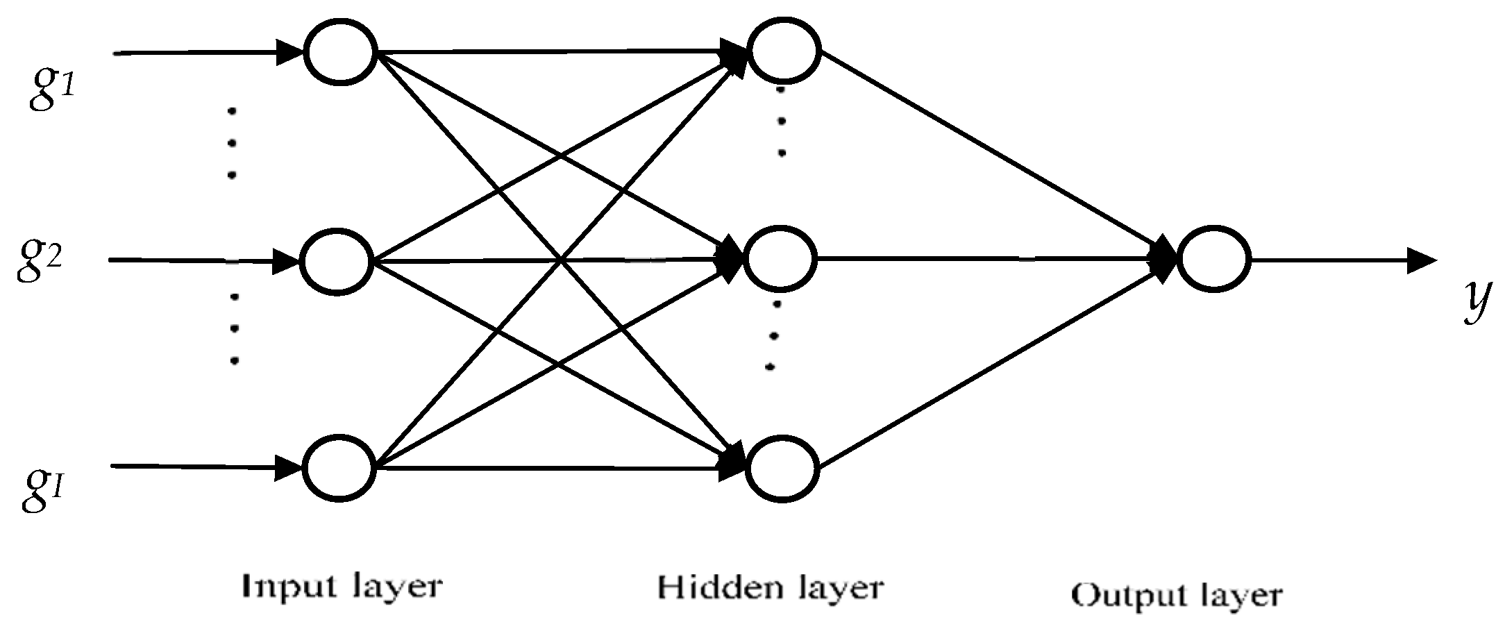
2.3. Artificial Neural Networks (ANNs)

ANNs, also popularly referred to as artificial neural systems, are efficient computing systems or relatively simple computational models founded on the neural organization of the brain with functional changing parameters to process information effectively. ANNs are distinctive and robust non-linear statistical data modeling networks wherein reasonably simple connections between inputs and outputs nodes alignments are established. According to Robert Hecht-Nielsen, the first inventor of the neurocomputer, a neural network can be defined as “a computing system made up of several simple, highly interconnected processing elements, which process information by their dynamic state response external inputs”. The processing elements are called neurons. The neuron is the special mathematical function that captures and organizes information according to the neural network architecture.

Some of the essential features or advantages of ANNs are [31,34,35,36].

• High-speed computation adeptness
• Global interconnection of network processing elements
• Robust distributed and asynchronous parallel processing
• High adaptability to non-linear input-data mapping
• Robust noise tolerance
• High fault tolerance utilizing Redundant Information Coding
• Robust in providing real-time operations
• High potential for hardware application
• Capable of deriving meaning from the imprecise or complicated dataset
• High capacity to learn, recall and generalize input data training pattern

3. Methodology

As mentioned earlier, the ANN model possesses many robust training algorithms and hyperparameters that can be explored to conduct proficient adaptive nonlinear statistical modelling over the classical logistic regression methods. This section contains the materials and method explored to develop the proposed MLPANN-based model with well-structured implementation network architecture, empowered with the right hyperparameter tuning algorithm for optimal predictive analysis of practical path loss data. The stepwise exploratory method explored to develop the proposed MLPANN-based model is highlighted as follows:

• Acquire the path loss datasets
• Preprocessing the dataset and splitting
• Obtain the MLP neural network model.
• Identify the adaptive learning algorithms for MLP neural network model training and testing
• Identify the modelling hyperparameters
• Select a hyperparameter tuning algorithm for the model (e.g., Bayesian optimization search, grid search, etc.).
• Obtain a set of the tuned best hyperparameter values.
• Train the model to obtain the best hyperparameter values combination.
• Appraise and validate the accuracy of the training process.
• Repeat the process to optimal configuration and best-desired results for the model.
• Engage the model with well-structured implementation network architecture, learning algorithm and set of the tuned best hyperparameter values to conductive predictive path loss modelling.

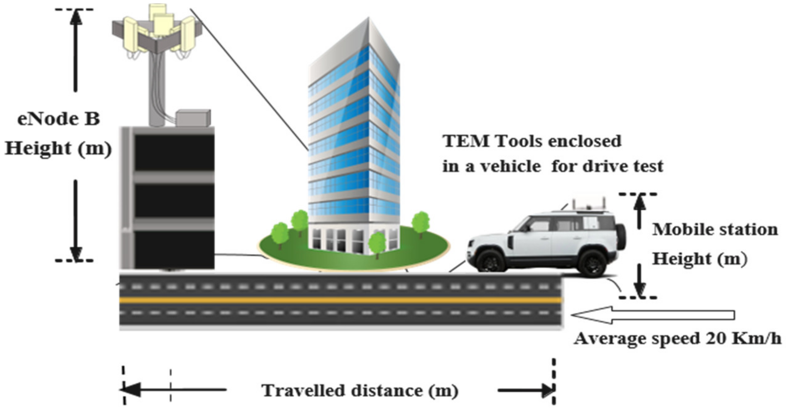
3.1. Data Collection

The field measurement was conducted to acquire live signal data around three Long Term Evolution (LTE) transceiver base station antennas for one year (i.e., 12 months). The measurement took one year to cater to the study locations’ seasonal variations and three LTE transceiver base station antennas operating at 2600 MHz with 10 MHz bandwidth [43]. The transceiver base station antennas (called NodeBs) are sectorized with 17.5 dBi gain and 43 dBm transmit power. The LTE network belongs to one of the major GSM/WCDMA/HSPA/LTE telecom service providers operating across major towns, villages and cities in Nigeria. The measurements were performed with field test tools with TEMS application tools for radio spectrum analysis. The test tools, some of which are displayed in Figure 1, include a Rover car, scanner, two Samsung mobile phones, and an HP lap, were explored to assess the performance of eNode B over the LTE radio air interface by connecting mobile phones directly to the Node B transmitters. To obtain the eNode B locations and delineate measurement data locations/information, the Global Positioning System (GPS) equipment was employed. The path loss data to be predicted are related to the acquired radio signal data by the measured path loss data where $P{L}_{mea}(\mathrm{dB})$, values have been obtained from the measured signal, RSRP (dBm) by Equation (1):

$$P{L}_{mea}(\mathrm{dB})=EIRP+G_A-RSR{P}_{meas}$$

(1)

With EIRP calculated as Equation (2):

EIRP = P_TX + G_TX − CL_TX

(2)

where G_TX and $G_A$ are the base station (BS) transmit antenna gain and receiver (MS) antenna gain, respectively, P_TX is the transmitted power, and CL_TX, denotes transmission cable loss, all in dB.

Table 1. Measurement Path Loss Computation Parameters.

Parameters	Site 1	Site 2	Site 3
BS Operation Transmitting Frequency (MHz)	2600	2600	2600
BS Antenna Height (m)	28	30	45
MS Antenna Height (m)	1.5	1.5	1.5
BS antenna gain (dBi)	17.5	17.5	17.5
MS antenna gain (dBi)	0	0	0
MS Transmit power (dB)	30	30	30
BS Transmit power (dB)	43	43	43
Transmitter cable loss (dB)	0.5	0.5	0.5
Feeder Loss (dB)	3	3	3

reveals some of the key BS antenna site parameters acquired during the field drive test for calculation.

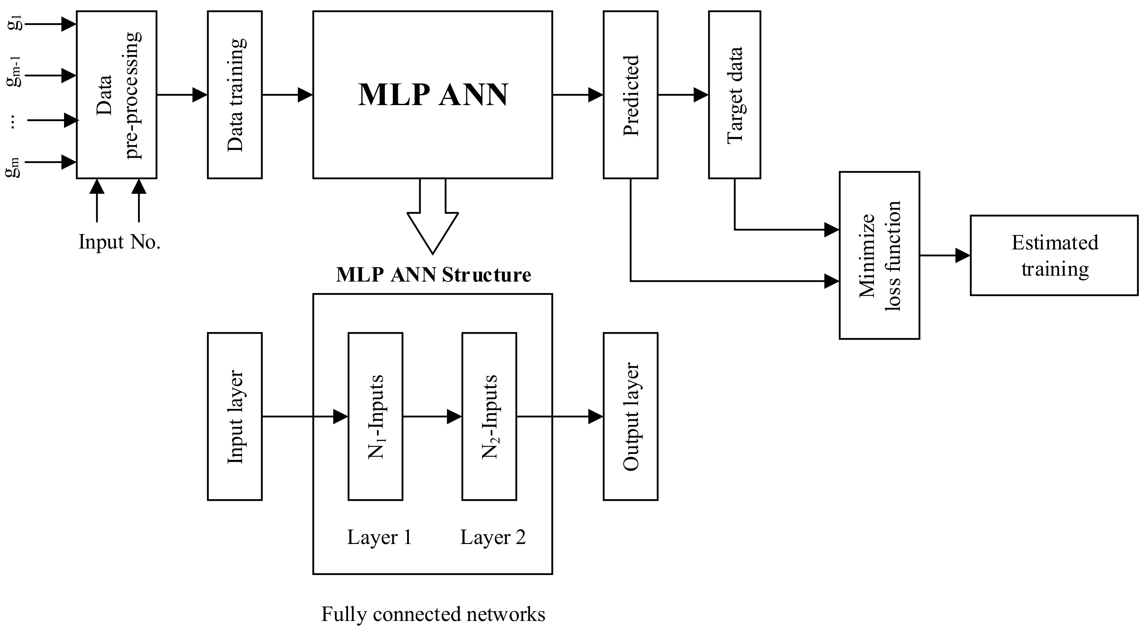
3.2. The MLP Neural Network Model

The first step towards effectively engaging neural networks for predictive modelling is to know the exact type you want to use and determine network architecture. This paper considers the most robust and special type of neural network: the multi-layer perceptrons (MLP). A single perceptron (LP) has limitations in terms of input-desired output mapping capability. This limitation is because it only contains a single neuron per adaptable synaptic weights and bias; thus, it is only proficient in catering to ridge-like function, notwithstanding the type activation function explored [42]. The above limitation can be catered to using an MLP neural network with more source nodes with data input and output layers sandwiched with hidden layers nodes. Multiple layers of neurons in the MLP network provide enhanced input-desired output mapping capability.

Figure 2 displays a structure of a classic feedforward MLP network model composed of $g_1^{}$,$g_2$,… $g_I$, inputs, and predicted output, ($y_1,y_2,\dots ,y_N)$ with k_h hidden nodes, h number. The respective weights connecting the input and hidden layer, as well as the weights connecting the hidden layer and the output layer, are designated by $w_{ij}^1$ and $w_{jn}^2$, while $C_j^{}$ indicates the hidden nodes thresholds. The network learns the correlation between input datasets and predicted output feedback by varying weight and bias values. Accordingly, the MLP network predicted output in correspondence to jth neurons with the kth node could be articulated as (3):

$${\widehat{y}}_n\left(t\right)={\displaystyle {\sum }_{j=1}^{k_h}{w}_j^2}{F}_{}\left({\displaystyle \sum _{}^{}{w}_{ij}^1{g}_i(t)+c_j}\right)$$

(3)

for $1\le n\prec m$, $1\le j\prec k_h$, $\left(w_j,j=0,1,\dots ,k_h\right)$, $\left(w_{ij},i=0,1,\dots ,m;j=0,1,\dots ,k_h\right)$

where:

m, h and k_h indicate the input node number, hidden node and hidden node number, respectively; i designate input to j hidden layer neuron.

The F (·) in Equation (1) denotes the sigmoid activation function, an import function usually utilized in the MLP network. It can be defined by Equation (4):

$$F(a)=\frac{1}{1+e^{-a}}$$

(4)

where F(x) is at all times in the range [−1, 1], with F(a) being a set of real numbers.

The weights $w_{ij}^1$ and $w_{jn}^2$, including the threshold $C_j^{}$, are unknown and thus can be chosen to update and reduce the error during prediction. The prediction error can be expressed by employing the expression (5):

$${\epsilon }_n=\frac{1}{2}{\displaystyle {\sum }_{n=1}{\left(y_n-{\widehat{y}}_n^{}\right)}^2}$$

(5)

where,

$y_n$ and ${\widehat{y}}_n$ represent the target (i.e., actual) data and their predicted output; and n = 1…, N, with N indicating the actual data sample number.

In MLP training, the error verve for assessing the network learning improvement related to convergence speed is the generalized aggregate error values. It is often computed using mean square error (MSE). The MSE can be obtained from the least square formation of Equation (6).

$$MSE=\frac{1}{N}{{\displaystyle \sum _{n=1}^N\left(y_n-{\widehat{y}}_n^{}\right)}}^2$$

(6)

In this work, the feedforward MLP network model explored for path loss predictive modelling is displayed in Figure 3.

3.3. MLP Modelling Parameters and Search Space

Hyperparameters are a special set of regulating parameters that the NN model utilizes for the adaptive learning process in data training and testing. The special parameters may be categorical, continuous or integer variables whose values range are usually lower and upper bounded. Thus, there exists several MLPs directly impacting the predictive modelling. They include the hidden layers number, neurons number in the hidden layer, transfer function, etc. A summarised description of the transfer function is given in the following subsection.

3.3.1. The Hidden Layers

Deciding the number of the hidden layers is one of the most important issues while investigating the neural network architecture for predictive modelling and data mining. Using too many hidden layers can result in poor generalization and complex neural network training. According to authors in [44,45,46,47], two hidden layers, combined with m output neurons, are adequate for a neural network to learn N data samples and produce negligibly minor errors.

Previous studies have examined the suitability of several machine models for path loss predictions as contained in [48,49,50]. The need to overcome the problems of empirical models when used for path loss predictions led to an artificial neural network [49]. ANN path loss prediction models were also more efficient and easier to deploy than deterministic models [51]. In [52,53], analyses of empirical models with different propagation features were performed, and the model with the lowest RMSE value was then compared with the prediction from ANN. The ANN-based path loss prediction model produced a much lower value of MSE upon validation. In [54], a multi-layer perceptron neural network was introduced for path loss prediction. The MLP network was then trained with a backpropagation algorithm. The MLP-based prediction was compared with predictions from analytical models, and the results indicated the former to be efficient for radio network planning and optimization.

ANN was also used for path loss prediction in urban areas [55]. The work explored the effect of the various input parameters and the environmental terrains on the robustness of the path loss prediction. One key finding from the study is that the accuracy of the signal prediction model increases with more input parameters: the greater the number of features, the greater the system’s accuracy. This trend is because machine learning algorithms thrive well with the availability of large datasets. The model is trained with the help of the data and, in this case, the input features. An ANN-based path loss model at 800 MHz and 1800 MHz introduced in [47,48] were input for longitude, latitude, distance, elevation, clutter height and elevation. The ANN method in [56] outperforms the Support Vector Machine (SVM)- and the Random Forest (RF)-based predictions.

In [57], an artificial neural network was used for path loss prediction in a smart campus environment at 1800 MHz. There were two hidden layers for this network, and the performance of the network outperforms the prediction made by using RF. Moreover, in [58,59,60], several machine learning-based prediction models were introduced for signal predictions for wireless sensor networks. The machine learning-based prediction model in [61,62] also produced the lowest values of RMSE when compared to the other analytical models in a wireless sensor network.

3.3.2. Neurons Number in the Hidden Layers

Determining the neurons number in the hidden layers remains an integral part of the inclusive neural network architecture. An inadequate neurons number in the hidden layers can lead to an underfitting problem. Underfitting arises once there are insufficient neurons number in the hidden layers to learn or detect the signals satisfactorily, especially in a multifaceted dataset.

On the other hand, using too many neurons can lead to overfitting problems. Overfitting occurs once the neural network contains too much information processing capacity problem. It can also result in excessive time increase during neural network training. The amount of training time can increase to the point that it is impossible to train the neural network adequately. It is evident that some give and take must be grasped between too few and too many neurons number in the hidden layers.

3.3.3. Transfer Function

The transfer function is a singular, monotonically increasing and differentiable function used for translating the input data signals to produce the final output signals of a neuron. The transfer function is fundamental to the concrete concept of neural networks mainly for two key reasons. First, without activation functions, the entire organization of the neural network will be similar to a typical linear function that cannot learn non-linear relationships. Second, transfer function styles and graces the main computation accomplished by neural networks.

3.3.4. Learning Rate

The learning rate is another vital hyperparameter that regulates or fine tunes the weights of NN in relation to the loss gradient. Its value must be cautiously chosen to support both optimization and generalization robustly. A too-large learning rate value can cause the entire learning process to jump over minima. Similarly, a too-small learning rate value can make the entire learning process too long to converge, resulting in it being trapped in negative and spurious local minima.

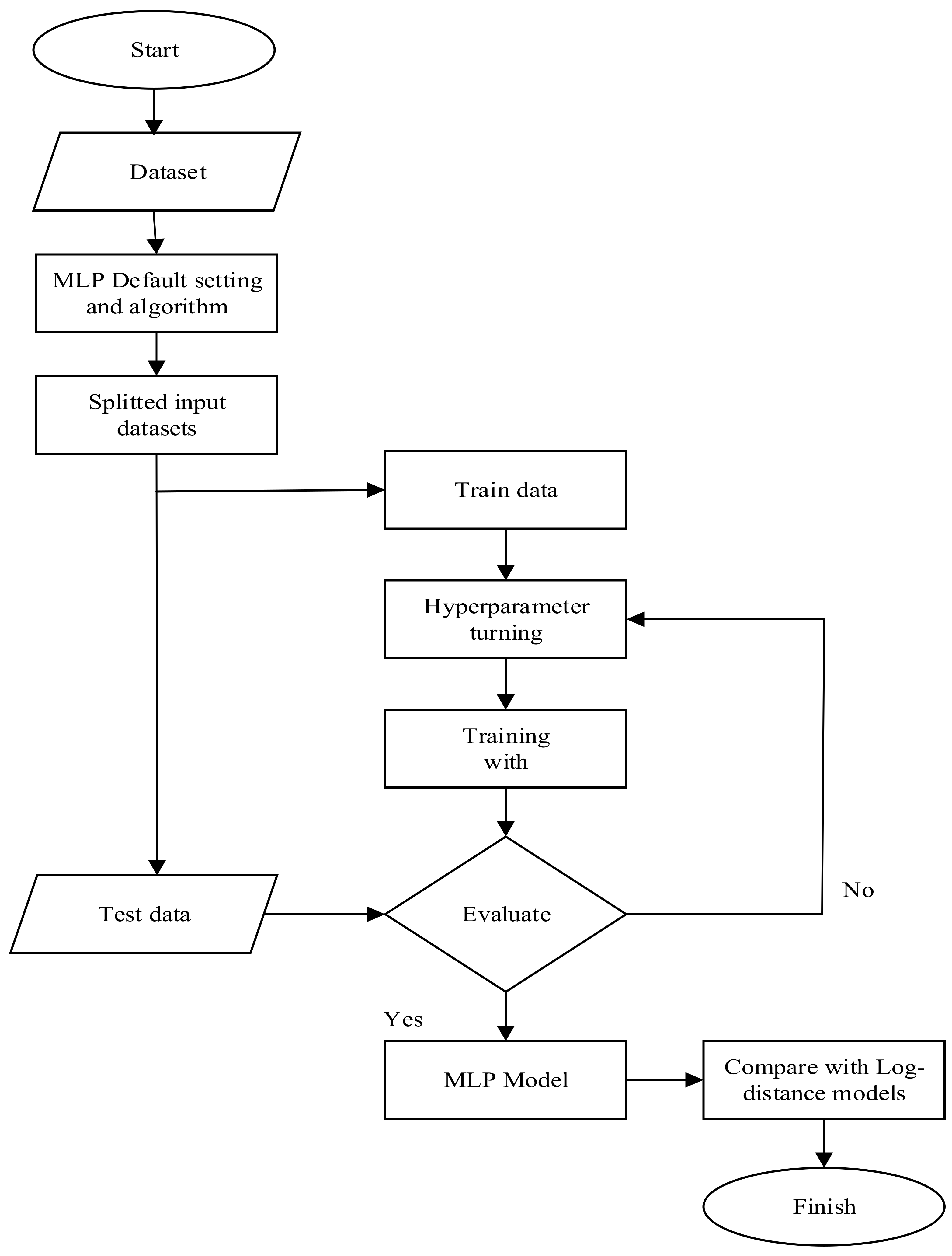
3.4. Hyperparameter Tuning

Hyperparameter tuning or optimization expresses the robust procedure of identifying and finding the best feasible values of hyperparameters for a machine learning model to attain the desired resultant modeling outcome. Popular hyperparameter tuning algorithms in the literature include random search, grid search and Bayesian optimization search. In this paper, the last two methods are considered. Grid search is a standard hyperparameter optimization technique wherein a list of critical parameters is selected with attached feasible values for each parameter, followed by training the model for every single blend and then choosing the values that yield the most desired resultant outcome. The Bayesian optimization method is a special sequential model-based optimization (also known as Bayesian optimization), utilizing the ‘Bayes Theorem’ to conduct an automatic hyperparameter search. Particularly, the Bayesian optimization search algorithm utilizes the upshot from the preceding iteration to select the next hyperparameter values.

3.5. MLP Learning Algorithms

The training algorithm used for a neural network system to learn and solve a problem is essential. The correct training algorithm from the available sundry types depends on diverse factors, including data sample size, task type, training time constraints, precision/accuracy requirements, etc. It is demanding to find out which training algorithm will produce the most satisfactory results. For example, suppose it is a predictive modelling task with function approximation. In that case, the dominant or most common ones are backpropagation training algorithms, which involve carrying out computations backwards over the network to fine-tune the weights and minimize performance error.

3.6. MLP Network Model Implementation Process

MATLAB is a distinctive programming language with a multi-exemplar numerical computing environment and a user interface. It provides easy matrix manipulation, graphical multi-domain simulation, figurative computing, creative functions plotting, excellent data mining, easy algorithms implementation, etc. MATLAB allows access to optional toolbox uses. The neural network toolbox has special tools for model-based design, implementation, visualization and simulation of neural networks. MATLAB is employed to encode the script files for the MLP network model predictive training, testing and quantitative evaluation in this work. The program code for conventional path loss calculation and assessment is also explored. The proposed MLP neural model consists of five input nodes and one output node. Flowchart for executing proposed predictive modelling with ANN while training and testing are shown in Figure 4.

As mentioned earlier, for practical and optimal application of MLP network for predictive modelling purposes, the right choice of the learning algorithm, and selection of the network processing elements such as the number of neurons, number of network layers and transfer functions, are crucial. For example, a network with insufficient neurons number in a hidden layer may fail to capture complex links between target output and input variables. Conversely, if the number of neurons allotted in the network hidden layer is too many, the network would likely follow the latent noise in the dataset owing to over-parameterization, and this, in turn, can lead to awkward generalization and poor predictive modelling of the original data [63,64]. Therefore, the determination of the hidden layers number and their number of neurons is performed by trial and random selection. However, for conciseness and the need to attain optimal neural network training and testing, the search for the required number of neurons and hidden layers in the network layers were narrowed down to 2–50 and 1–3, respectively.

Generally, if a particular algorithm performs well during the dataset training but flops in the aspect of generalization, we refer to it as overfitting. To improve generalization (or prevent overfitting) during the path loss data training with each of the NN algorithms, we employed input/target transformations and early stopping techniques. Thus, the inputs and targets datasets were scaled to reside in the range [−1, 1] to enhance training and testing speed. Moreover, the early stopping measures were engaged for training and testing to avoid overtraining, eliminate contemptuous impact stimulated by the initial values, and develop robust adaptive predictive ability. Although many learning algorithms are available for MLP neural network training and testing in MATLAB software, it is demanding to identify which algorithm works best for a given predictive modelling problem concerning convergence speed and accuracy [16]. Therefore, an exhaustive search is employed in this study to accelerate the convergence and evaluate the impact of all the available learning algorithms during network training. The respective learning algorithms assessed to develop an optimal MLP network predictive model and their weight adaptation techniques are listed in

Table 2. Respective MLP Network Learning Algorithm.

Learning Algorithm	Weight Adaptation	Training Acronym
Levenberg–Marquardt (lm)	The weight of the lm algorithm is updated via: $w_{q+1}=\hspace{0.17em}{w}_q-{(H^{’}+\eta I)}^{-1}\nabla {\epsilon }_q$ where the Hessian matrix, $H^{’}=J^{T}J$.	trainlm
Bayesian Regularization (br)	The br approach involves the modification of the performance function, ${\epsilon }_q$ plus regularisation term $F_{}(w)=\beta {\epsilon }_q^{}+\alpha {\epsilon }_w$ where $\beta$ & $\alpha$ are special function parameters and a regularisation term, ${\epsilon }_w={‖w‖}^2$	trainbr
Polak–Ribiere Conjugate Gradient (cgp)	The weight of cgp algorithm is updated by: $w_{q+1}=w_q+a_q{p}_q$ With $p_q$ = $-g_q+b_q{p}_{q-1}$ and $b_q=\frac{∆g_{{}_{q-1}}^T{g}_q^{}}{g_{q-1}^T{g}_{q-1}^{}}$	traincgp
Fletcher-Powell Conjugate Gradient (cgf)	The weight of scg algorithm is updated by: $w_{q+1}=w_q+a_q{p}_q$ With $p_q$ = $-g_q+b_q{p}_{q-1}$ and $b_q=\frac{g_{{}_{q-1}}^T{g}_q^{}}{g_{q-1}^T{g}_{q-1}^{}}$	traincgf
Scaled Conjugate Gradient (scg)	The weight of scg algorithm is updated by: $w_{q+1}=w_q+a_q{p}_q$	trainscg
Resilient Backpropagation (rp)	With RP algorithm, weight update is by $w_{q+1}=\hspace{0.17em}{w}_q-sign\left(\frac{∆{\epsilon }_q}{∆w_q}\right).∆(q)$ where $∆(q)$ = individual step size for weight adaptation	trainrp
BFGS Quasi-Newton (bfg)	bfg weight update is accomplished via $w_{q+1}=w_q-H^{-1}{g}_q$ where $H_q^{-1}$ indicates the Hessian matrix inversion on iteration q.	trainbfg
Conjugate gradient with Powell/Beale Restarts (cgb)	The cgb employs update search direction by: $g_{q-1}{g}_q=0.2{‖g_q‖}^2$	traincgb
Gradient Descent with Adaptive Learning Rate (gda)	gda weight update is accomplish via $w_{q+1}=\hspace{0.17em}{w}_q+{\frac{∆\epsilon }{{\eta }_{q+1}∆w}}_q$ where $\alpha$ indicates the user-defined momentum factor and it ranges from 0 to 1	taingda
Gradient Descent Variable Learning Rate (gdx)	With gdx algorithm, weight update is by $w_{q+1}=\hspace{0.17em}{w}_q{\eta }_{q+1}-sign\left(\frac{∆{\epsilon }_q}{∆w_q}\right).∆(q)$ where $∆(q)$ = individual step size for weight adaptation and ${\eta }_q$ = variable learning rate	traingdx
One Step Secant (oss)	With oss algorithm, weight update is by $w_{q+1}=\hspace{0.17em}{w}_q-H_q^{-1}{g}_q$ where $H_q$ = Hessian matrix (2nd derivatives)	trainoss
Gradient Descent with Momentum (gdm)	gdm weight update is accomplish via $w_{q+1}=\hspace{0.17em}{w}_q-\eta g_q+\alpha {\frac{∆\epsilon }{∆w}}_{q-1}$ where $\alpha$ indicates the user-defined momentum factor and it ranges from 0 to 1	traingdm
Gradient Descent (gd)	With gm algorithm, weight update is by $w_{q+1}=\hspace{0.17em}{w}_q-\eta g_q$ where ${\eta }_{}$ = learning rate	traingd

. The target of the weight adaptation is to determine the optimum weight update for the input-output data array pair during training.

4. Results and Discussions

As mentioned earlier, many factors directly impact the development of an excellent back-propagation neural network predictive model, especially with a trial and error method, as adopted in this work. They include training algorithm, hidden layers number, neurons number in the hidden layer, transfer function, momentum term, learning rate, etc. Here, the concentration is on the training algorithm, hidden layers number and neurons number in the hidden layer. To obtain the predictive path loss modelling results, first we divided the path loss data into portions and employed the grid search-based hyperparameter tuning method to generate configurations for the parted data chunks for training and testing. The performance results of the proposed method were evaluated and reported for each machine learning algorithm described in Table 1, using Mean Absolute Error (MAE), Mean Square Error (MSE), Root Mean Square Error (RMSE), Coefficient of Efficiency (COE), Correlation Coefficient (R) and Standard Deviation Error (STD) [65].

Secondly, the predictive path loss modelling was conducted for three study locations using the standard Bayesian optimization for hyperparameter tuning. The results were compared to our first results using the grid search-based hyperparameter tuning method.

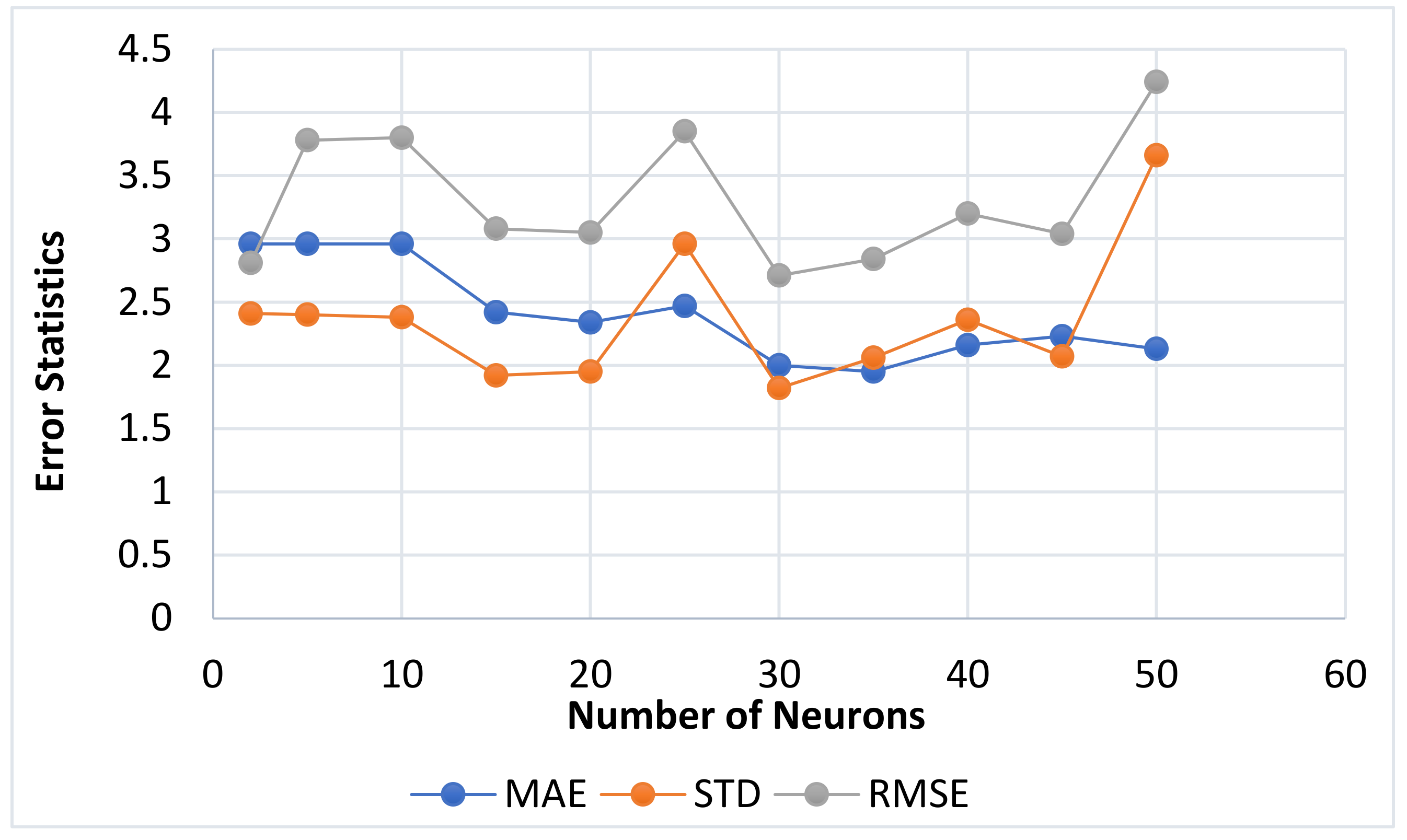
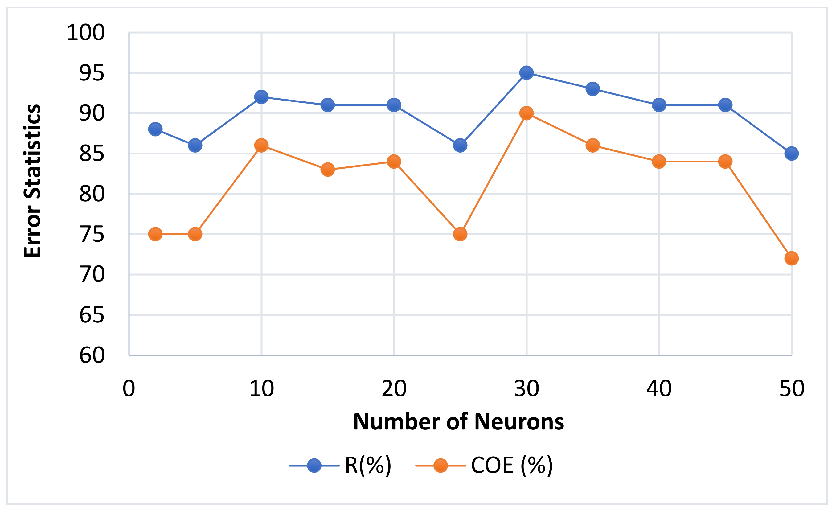
4.1. Neurons Number Impact

Determining the neurons number in the hidden layers also remains integral in the inclusive neural network architecture. An inadequate neurons number in the hidden layers can lead to an underfitting problem. Underfitting arises once there is insufficient neuron number in the hidden layers to satisfactorily learn or detect the signals, especially in a multifaceted dataset. On the other hand, making use of too many neurons can lead to overfitting problems. Overfitting takes place once the neural network contains too much information processing. It can also result in excessive time increase during neural network training. The amount of training time can increase to the point that it is impossible to adequately train the neural network. It is very clear at this point that some give and take must be grasped between too few and too many neurons number in the hidden layers. Accordingly, by starting with the fastest training algorithm, which is Levenberg–Marquardt (lm), the network was trained and tested with 2, 5, 10, 15, 20, 25, 30, 35, 40, 45 and 50 neurons. This is to ascertain their incremental impact on its performance.

Table 3. Neurons Number impact on MLP Network Predictive Modelling with LM.

	Training		Testing		Overall Performance
No of Neurons	MSE	R	MSE	R	MAE	STD	RMSE	R	COE (%)
2	12.91	0.8874	23.22	0.7913	2.96	2.41	3.81	0.8637	75
5	12.22	0.8643	11.93	0.9205	2.92	2.40	3.78	0.8637	75
10	7.32	0.9320	8.01	0.8900	2.96	2.38	3.80	0.9251	86
15	7.95	0.9229	15.72	0.8339	2.41	1.92	3.08	0.9117	83
20	8.59	0.9247	13.79	0.9186	2.34	1.95	3.05	0.9148	84
25	7.83	0.9296	53.08	0.4865	2.47	2.96	3.85	0.8635	75
30	5.08	0.9591	17.06	0.8558	2.00	1.82	2.71	0.9499	90
35	4.88	0.9531	22.45	0.8482	1.95	2.06	2.84	0.9255	86
40	7.29	0.9360	14.31	0.7973	2.16	2.36	3.20	0.9132	84
45	7.95	0.9315	11.06	0.8257	2.23	2.07	3.04	0.9143	84
50	3.62	0.9673	21.07	0.7624	2.13	3.66	4.24	0.8498	72

, Figure 5 and Figure 6 display the detailed overall predictive performance of each neurons number using different error statistics. As seen in Table 3, it was expected that a continuing increase in neurons number per layer would result in an upturn in the resolution of the neural network prediction fitting pattern to the measured loss data. At 30 neurons per layer, the neural network model had a good enough fit to the measured loss data with an MAE value of 2, RMSE value of 2.71, STD value of 1.82, R-value of 95 (%) and COE value of 90 (%). Increasing the neuron number to 50 showed no performance improvement, as seen in Figure 6.

4.2. Transfer Function Impact

The transfer function is a singular monotonically increasing and differentiable function used for translating the input data signals to produce the final output signals of a neuron. The transfer function is fundamental to the concrete concept of neural networks mainly for three key reasons. Firstly, without activation functions, the entire organization of the neural network will be similar to an ordinary linear function that cannot learn non-linear relationships. Secondly, transfer function styles grace the main computation accomplished by neural networks. Thirdly, transfer functions possess the proclivity to boost the learning rate and formation patterns in datasets. Thus, the choice of the right transfer (activation) function also positively influences the performance of the NN training algorithm.

Table 4. Transfer Functions used for network training/testing and their performance.

	Training		Testing		Overall Performance
Transfer Function	MSE	R	MSE	R	MAE	STD	RMSE	R
purelin	19.74	0.8614	18.29	0.8692	3.36	2.65	4.28	0.8636
tansig	6.82	0.9366	26.07	0.7865	2.19	2.45	3.29	0.9073
logsig	4.62	0.9594	23.09	0.7812	2.15	2.30	3.15	0.9106
purelin-purelin	20.33	0.8715	13.09	0.8964	3.59	2.75	4.52	0.8637
purelin-tagsig	7.83	0.9325	12.20	0.8539	2.38	1.80	2.99	0.9173
purelin-logsig	9.18	0.9173	20.24	0.8755	2.52	2.02	3.24	0.9026
tansig-tansig	3.18	0.9697	20.17	0.8643	1.82	1.89	2.63	0.9365
tansig-logsig	3.23	0.9697	23.65	0.8094	1.82	2.18	2.84	0.9266
tansig-purelin	6.39	0.7622	10.28	0.6907	2.04	1.82	2.73	0.9315
logsig-logsig	4.82	0.9511	10.31	0.9382	1.76	1.63	2.40	0.9290
logsig-tansig	3.97	0.9669	12.96	0.8467	1.60	1.70	2.34	0.9499
logsig-pureline	6.01	0.9430	16.45	0.8471	2.18	1.91	2.90	0.9222
purelin-purelin-purelin	13.07	0.8804	18.34	0.8413	2.93	2.39	3.78	0.8637
tansig-tangsig-tansig	5.87	0.9487	8.89	0.9181	1.88	1.78	2.59	0.9283
tansig-tansig-purelin	6.38	0.9337	17.89	0.8607	2.17	2.06	2.76	0.9200
tangsig-tansig-logsig	5.11	0.9568	8.98	0.8907	1.92	1.93	2.72	0.9318
logsig-logsig-logsig	7.18	0.9358	13.86	0.9187	2.15	1.85	2.83	0.9285
logsig-logsig-purelin	9.12	0.9238	98.48	0.6384	2.91	4.03	4.97	0.8049
logsig-tansig-tansig	5.34	0.9489	7.52	0.9429	2.18	1.92	2.90	0.9245
logsig-tansig-logsig	6.90	0.9428	3.97	0.9467	1.98	1.75	2.67	0.9340
tansig-logsig-tansig	6.53	0.9433	3.68	0.9468	1.97	1.56	2.47	0.9445
logsic-tansig-purelin	6.92	0.9392	11.34	0.9093	2.09	2.02	2.90	0.9222
purelin-logsig-tansig	25.57	0.8583	25.94	0.8707	3.28	3.58	4.86	0.8597

presents the list of sigmoid transfer functions employed in this study to ascertain the stability of the proposed neural network model. The performance of sigmoid transfer functions in terms of MAE, MSE, RMSE, R and STD are also displayed in Table 4. The standard deviation (STD) statistics with one, two and three layers of training are given in Figure 7, and the Root Mean Error performance statistics with one, two and three layers of training are shown in Figure 8.

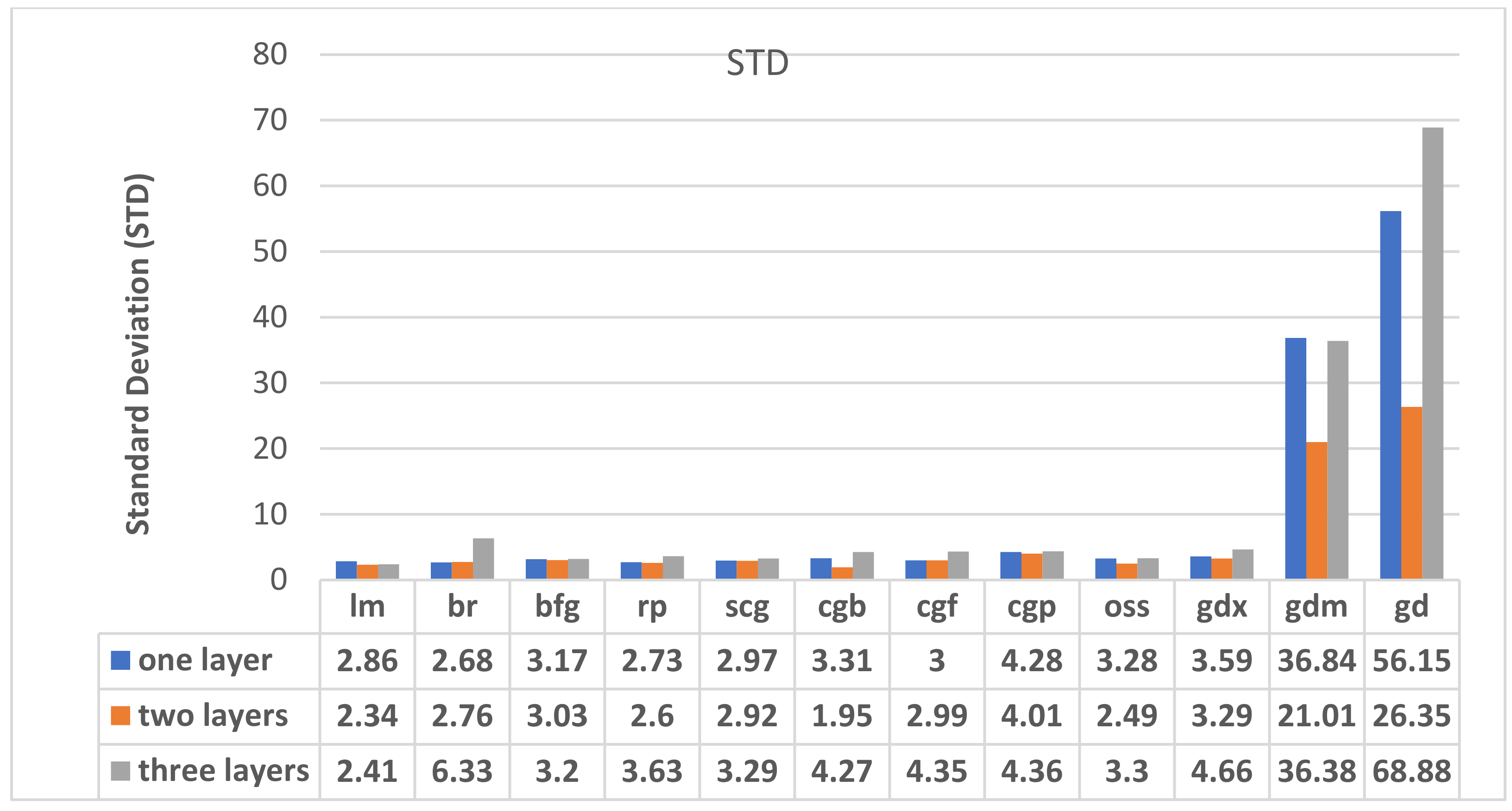
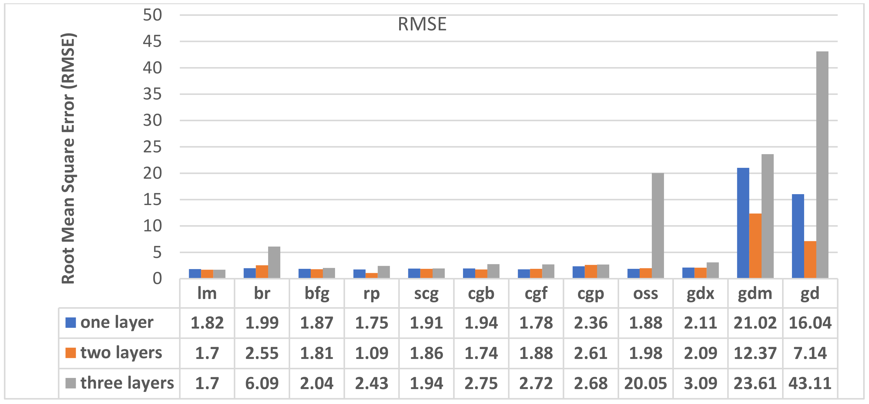
4.3. Training Algorithm and Hidden Layers Number Impact

The learning algorithm and hidden layers number also significantly impact the success of the neural network in coming up with a healthy predictive model. Therefore, deciding on the number of the hidden layer is one of the most important issues that come up while investigating the neural network architecture for predictive modelling and data mining. Using too many hidden layers can result in poor generalization and complex neural network training. According to the work [31], two hidden layers, combined with m output neurons, are adequate for a neural network to learn N data samples and produce negligibly small errors.

Here, the impact of many learning algorithms has been studied with one, two and three hidden layers numbers. Interestingly, results reveal that the two-layered network is superior to one-layered and three-layered layer network for all the 12 learning algorithms investigated. Interestingly, results show that the neural network architecture trained using lm (i.e., the Levenberg–Marquardt training algorithm) with two hidden-layer sizes and logsig-transit transfer function gave the best performance.

Table 5. Learning Algorithm and Hidden Layers Number impact on MLP Network.

		Training		Testing		Overall Performance
Training Algorithm	No of Hidden Layers	MSE	R	MSE	R	MAE	STD	MSE	R
lm	1	7.65	0.9359	11.55	0.9033	2.20	1.82	2.86	0.9248
	2	3.97	0.9669	12.96	0.8467	1.60	1.70	2.34	0.9499
	3	3.94	0.9632	9.31	0.9311	1.71	1.70	2.41	0.9473
Br	1	3.72	0.9660	26.59	0.7560	1.79	1.99	2.68	0.9340
	2	0.57	0.9953	47.07	0.7562	1.05	2.55	2.76	0.9408
	3	0.92	0.9919	25.68	0.3075	1.73	6.09	6.33	0.7557
Bfg	1	7.88	0.9252	14.88	0.9070	2.56	1.87	3.17	0.9076
	2	9.12	0.9092	12.92	0.8869	2.42	1.81	3.03	0.9149
	3	10.04	0.9159	10.93	0.8425	2.45	2.04	3.20	0.9045
Rp	1	7.68	0.9316	5.03	0.9601	2.09	1.75	2.73	0.9323
	2	4.38	0.9339	17.02	0.9123	1.90	1.09	2.60	0.9456
	3	5.03	0.9052	28.59	0.8816	2.69	2.43	3.63	0.8755
Scg	1	7.85	0.9282	11.08	0.8608	2.26	1.91	2.97	0.9185
	2	6.69	0.9373	13.52	0.7531	2.26	1.86	2.92	0.9209
	3	11.16	0.8951	9.65	0.8951	2.66	1.94	3.29	0.9005
Cgb	1	9.01	0.9168	14.75	0.8882	2.49	1.94	3.31	0.9089
	2	8.30	0.9293	8.89	0.9233	2.36	1.74	1.95	0.9202
	3	16.36	0.8460	29.72	0.8814	3.26	2.75	4.27	0.8510
Cgf	1	8.44	0.9186	12.65	0.9079	2.42	1.78	3.00	0.9165
	2	9.15	0.9152	8.93	0.9204	2.33	1.88	2.99	0.9168
	3	17.84	0.8274	21.14	0.8596	3.39	2.72	4.35	0.8449
Cgp	1	18.22	0.8496	23.49	0.7818	3.57	2.36	4.28	0.8426
	2	17.19	0.8472	11.26	0.9039	3.05	2.61	4.01	0.8482
	3	38.02	0.7463	36.79	0.7099	3.06	2.61	4.00	0.7486
Oss	1	9.53	0.9167	12.55	0.8703	2.70	1.88	3.28	0.9015
	2	9.06	0.9161	9.77	0.9116	2.49	1.98	2.49	0.9055
	3	10.16	0.9101	16.90	0.8084	2.59	20.05	3.30	0.8984
Gdx	1	11.82	0.8805	15.02	0.8584	2.91	2.11	3.59	0.8794
	2	9.59	0.9060	18.15	0.8430	2.54	2.09	3.29	0.8982
	3	18.60	0.8286	12.07	0.8252	3.50	3.09	4.66	0.8113
Gdm	1	1.42 × 103	0.8008	1.26 × 103	0.7041	30.26	21.02	36.84	0.7870
	2	447.60	0.7801	571.30	0.5385	16.97	12.37	21.01	0.8034
	3	1.22 × 103	0.4340	1.5 × 103	1.5 × 103	26.67	23.61	36.38	0.4504
Gd	1	2.94 × 103	0.7238	3.08 × 103	0.5882	53.81	16.04	56.15	0.6286
	2	655.14	0.8583	724.47	0.8268	25.67	7.14	26.35	0.8124
	3	468.86	0.7885	433.89	0.7589	53.72	43.11	68.88	0.7890

displays detailed network training/testing error statistics results and hidden layer numbers for each learning algorithm.

4.4. Performance of Grid Search Algorithm and Bayesian Optimisation Search Algorithm for Hyperparameter Tuning

The hyperparameter tuning process has a weighty influence on neural network learning performance. Given the computational resources requisite, the hyperparameters of high relevance receive superior usage in the hyperparameter tuning process. Hyperparameters with a more robust influence on weights are more effective during neural network training. Thus, the appropriate choice of hyperparameters selected for neural network model training influences the network training and performance.

As displayed in

Table 6. Comparison of Hyperparameter Tuning algorithm performance with Grid Search and Bayesian Optimisation search.

		Training		Testing		Overall Performance
Hyperparmeter Tuning Algorithm	MLP Algorithm	MSE	R	MSE	R	MAE	STD	MSE	R
Grid Search	lm	3.97	0.9669	12.96	0.8467	1.60	1.70	2.34	0.9499
	br	0.57	0.9953	47.07	0.7562	1.05	2.55	2.76	0.9408
Bayessian Optimisation search	lm	5.20	0.9565	16.73	0.8355	2.29	4.90
	br	3.52	0.9669	18.84	0.8567	3.40	4.24

, the proposed MLP neural network model results with grid search algorithm-based hyperparameter tuning (optimization) are compared with those obtained using the traditional Bayesian optimization search-based hyperparameter tuning approach for path loss data predictive analysis using location one as a case study. We have reported the results attained for lm and br learning for brevity. While the grid search-based hyperparameter tuning performs an in-depth and comprehensive search on the hyperparameters in a stepwise manner as set specified by users with limited search space, the Bayesian search-based hyperparameter tuning performs a sequential-based search on the hyperparameters via several trials, without the user having preliminary information of the hyper-parameters distribution. From the results in Table 6, it is clear that the proposed MLP neural network model with grid search algorithm-based hyperparameter tuning outperforms the ones obtained using Bayesian Optimization search-based hyperparameter tuning. Next, Section 4.5 is to apply the proposed MLP neural network model with grid search algorithm-based hyperparameter tuning for detailed predictive path loss analysis across the three study locations.

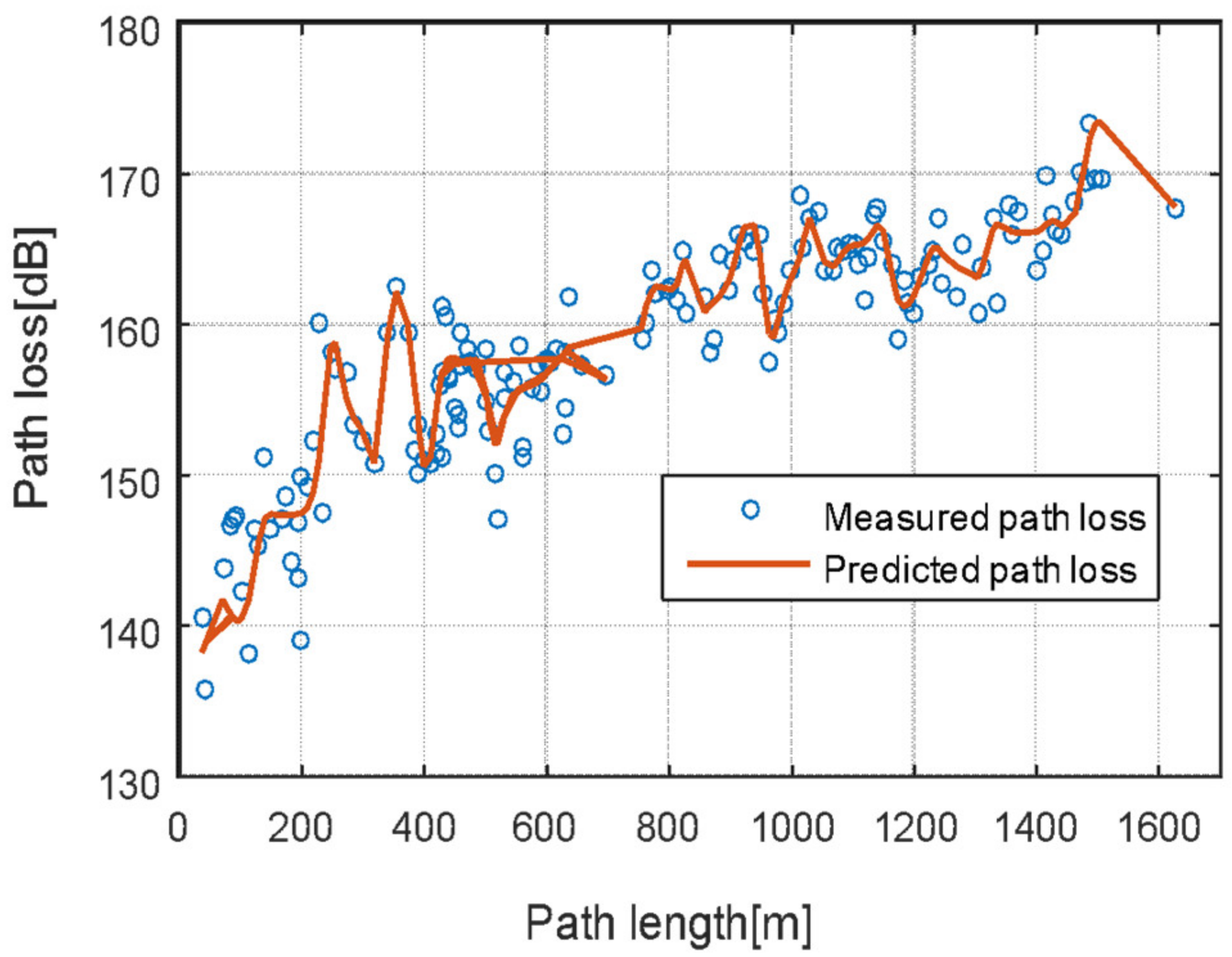
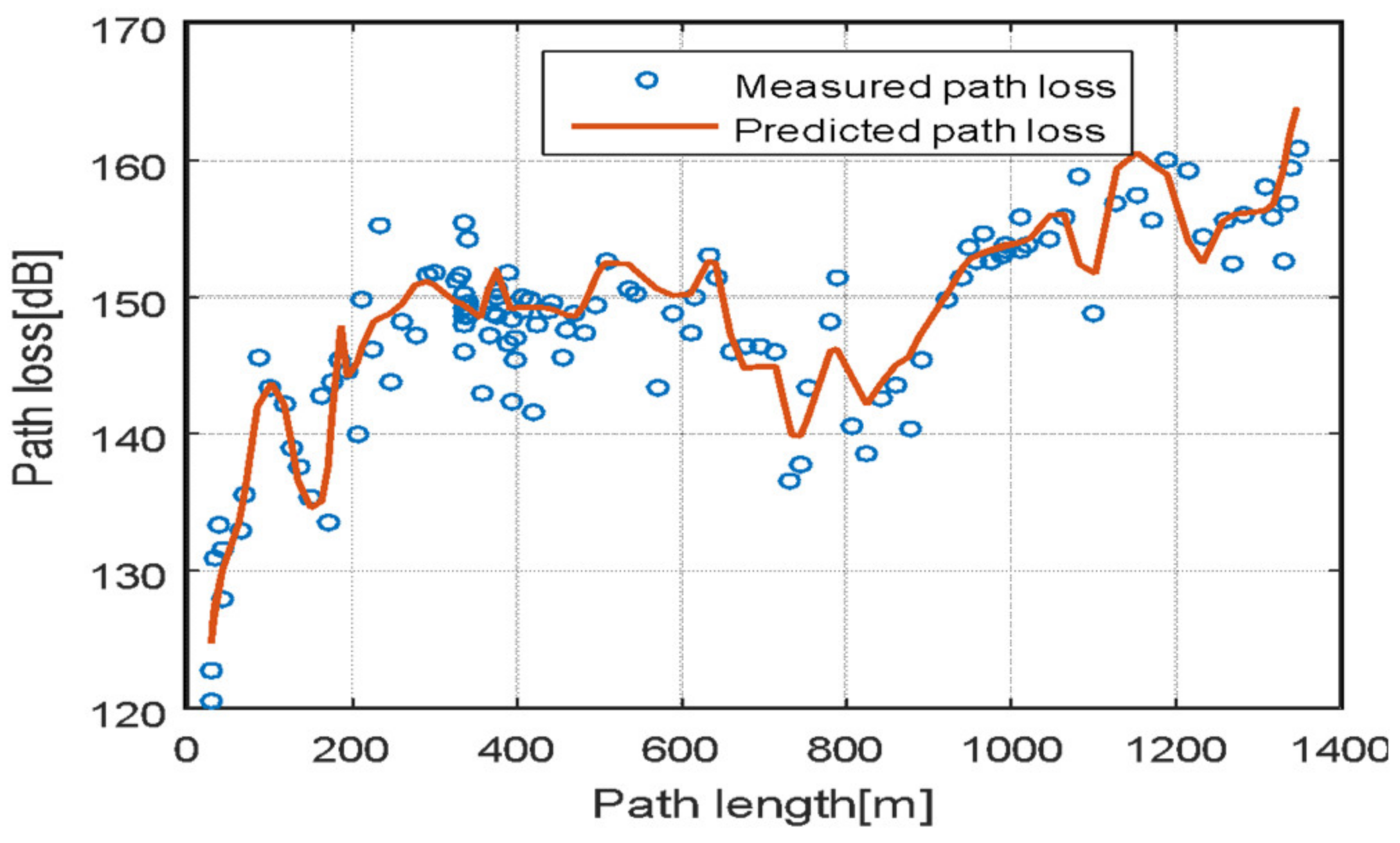
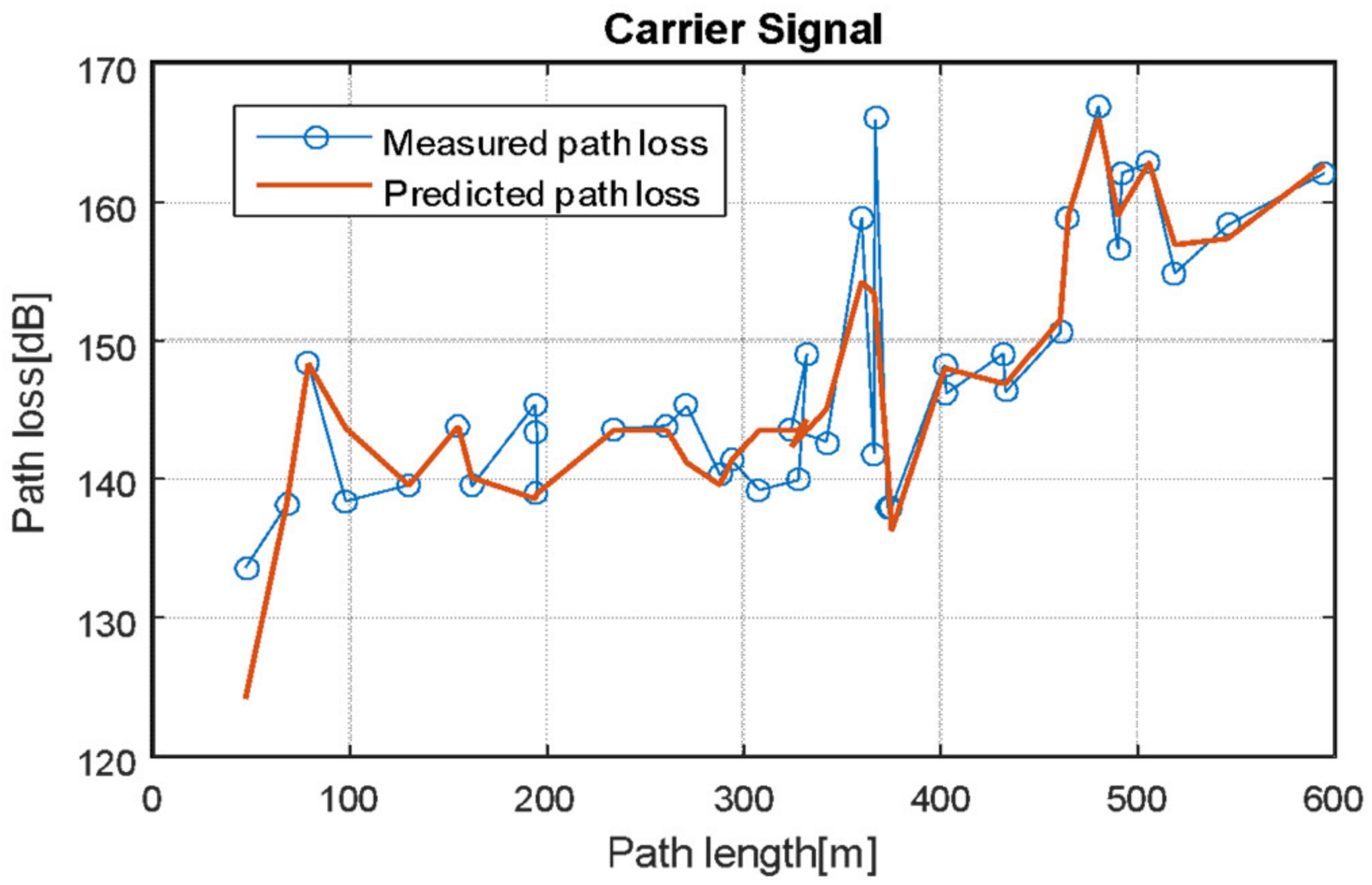
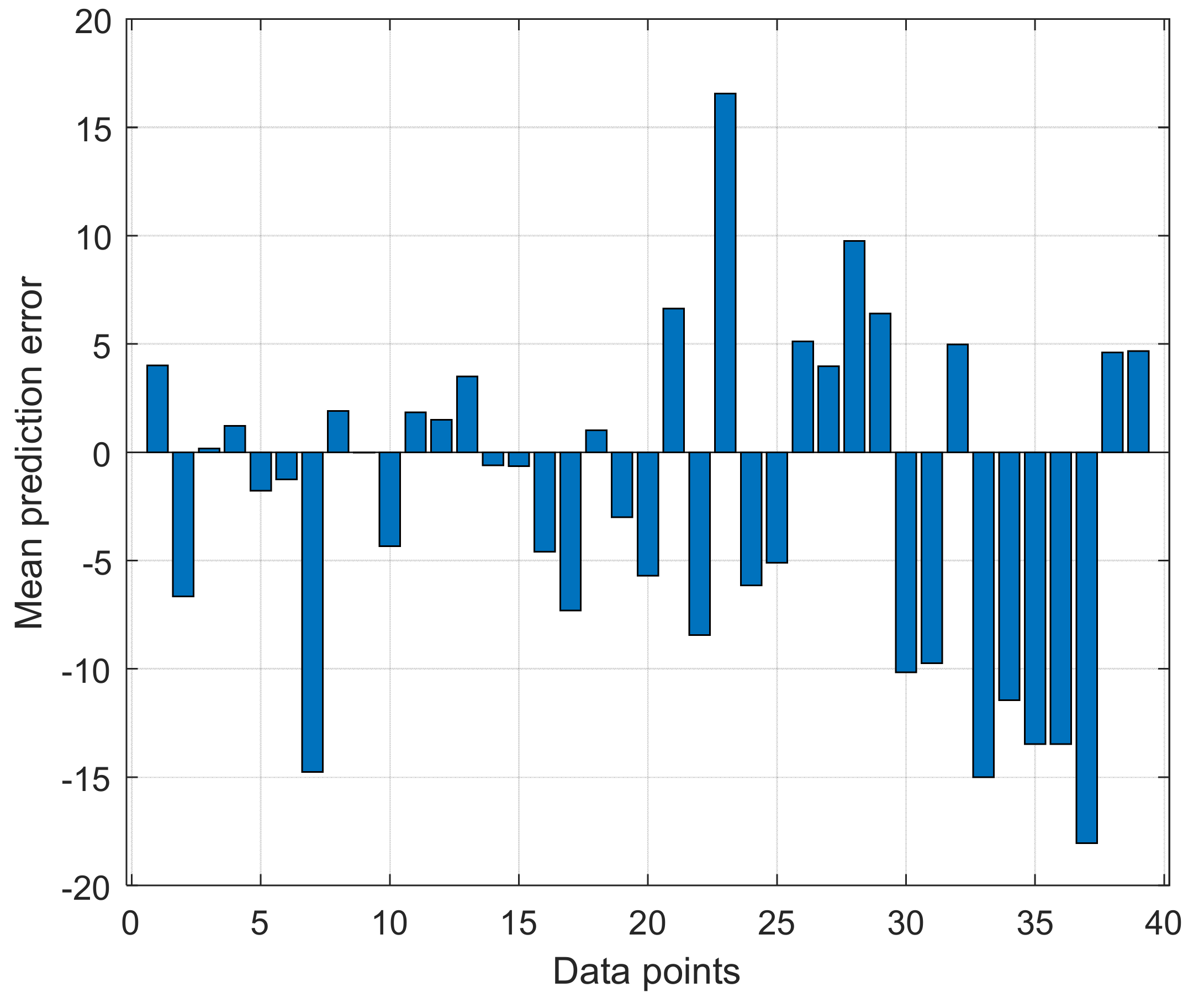
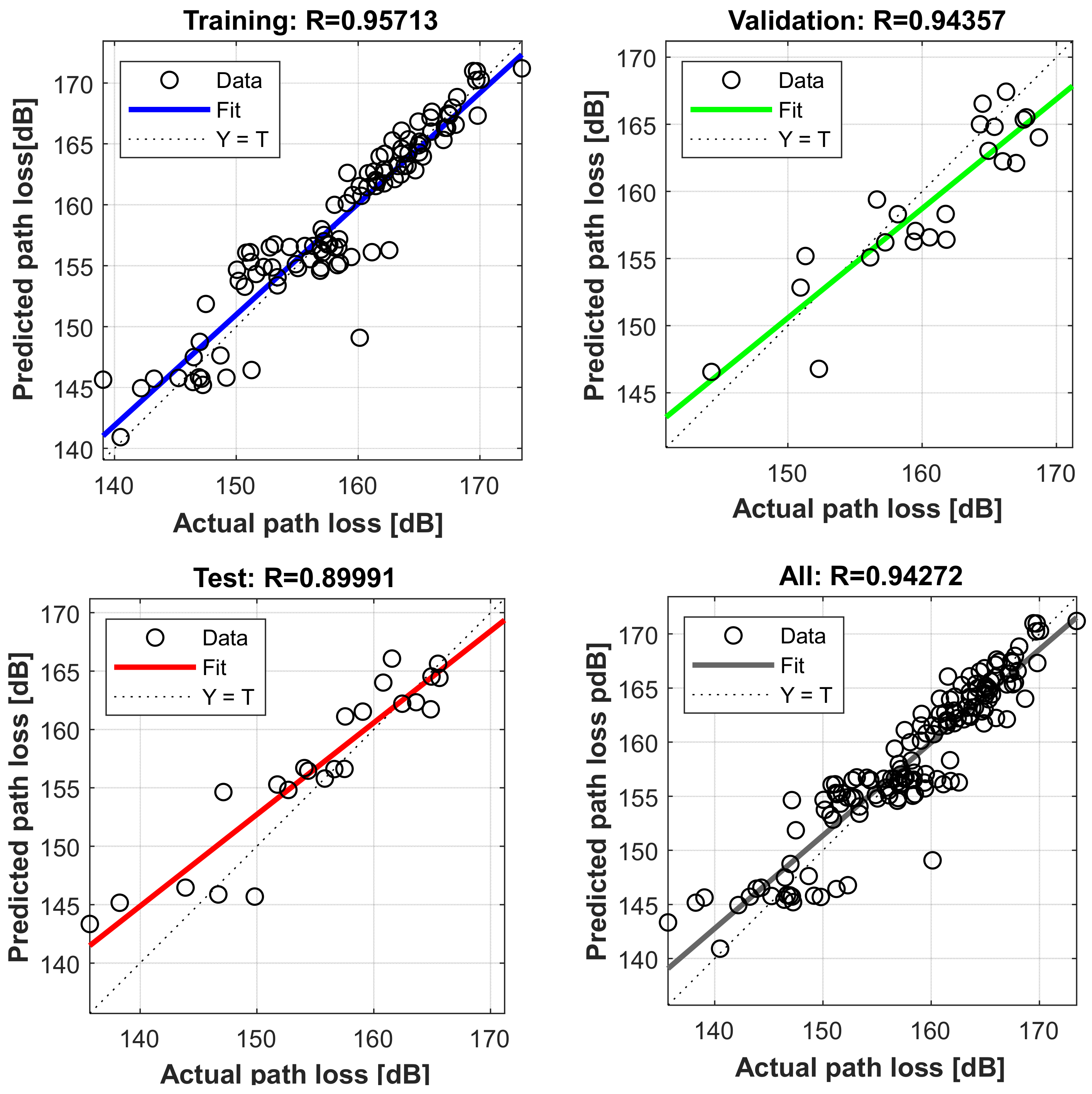
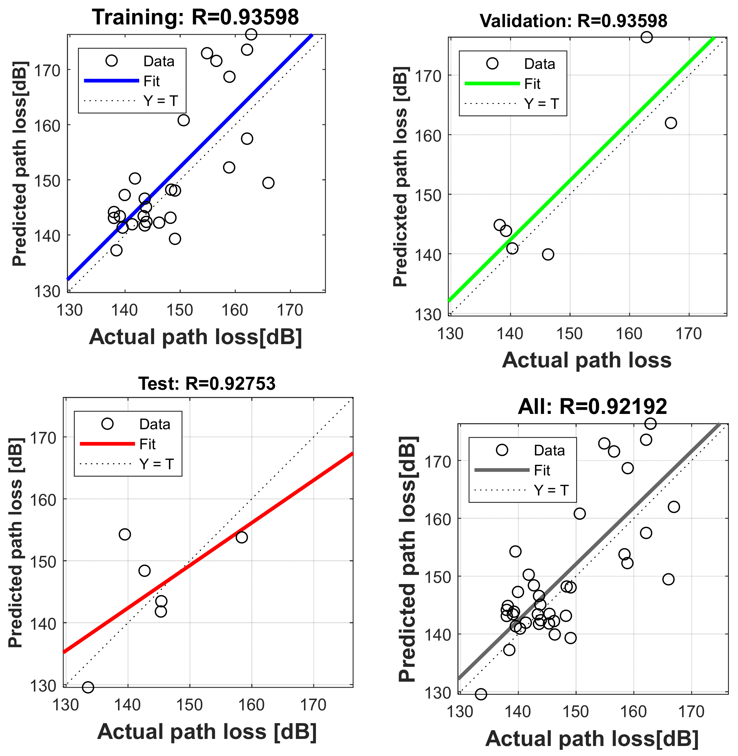
4.5. Evaluation of Proposed Neural Network Model at Different Locations

The evaluation results of the proposed neural network model at different study locations are presented as follows. Figure 9, Figure 10 and Figure 11 show the proposed neural network model prediction with measured path loss data configured with the Levenberg–Marquardt training algorithm, two hidden-layer sizes and logsig-transig transfer function—the prediction performance of the developed neural network model in terms of R and MSE values. The R-value measures the prediction correlation between outputs (predicted loss data) and targets (actual loss data). The closeness of the R-value to 1 corresponds to a high positive correction. Otherwise, it is poorly correlated. Figure 12, Figure 13 and Figure 14 are plotted R values between the predicted loss data and the actual loss values for sites 1 to 3 during training, validation and testing with neural networks. The R-values obtained from the plots are 0.97, 0.93 and 0.94 for site 1, 0.92, 0.93 and 0.94 for site 2 and 0.91, 0.93, 0.96, 0.94 for site 3. The performance plots in Figure 15, Figure 16 and Figure 17 indicate that the MSE becomes smaller with the epoch number (one complete training/testing/validation cycle). The word ‘epoch’ is used here to mean a special hyperparameter term that defines the number of times (in terms of iteration) that the NN algorithms undergo during the entire data training duration. The error of test and validation display similar characteristics while predicting the measured loss across sites 1 to 3. Specifically, the validation MSE error shows that the proposed neural network model would not generalize well or fit the measured loss data well if trained further than 4, 8 and 8 epochs. The mean prediction error along measurement data points in sites 1, 2 and 3 are presented in Figure 18, Figure 19 and Figure 20.

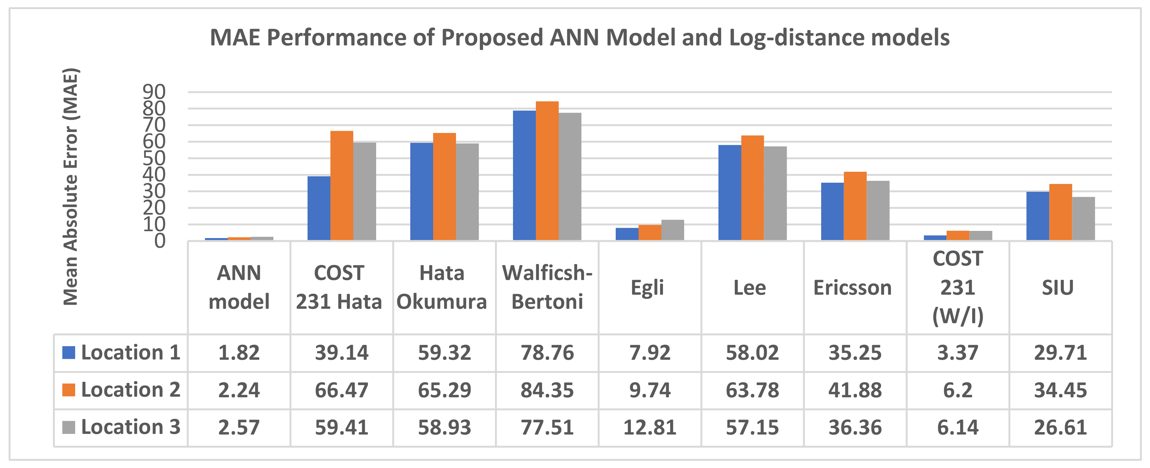
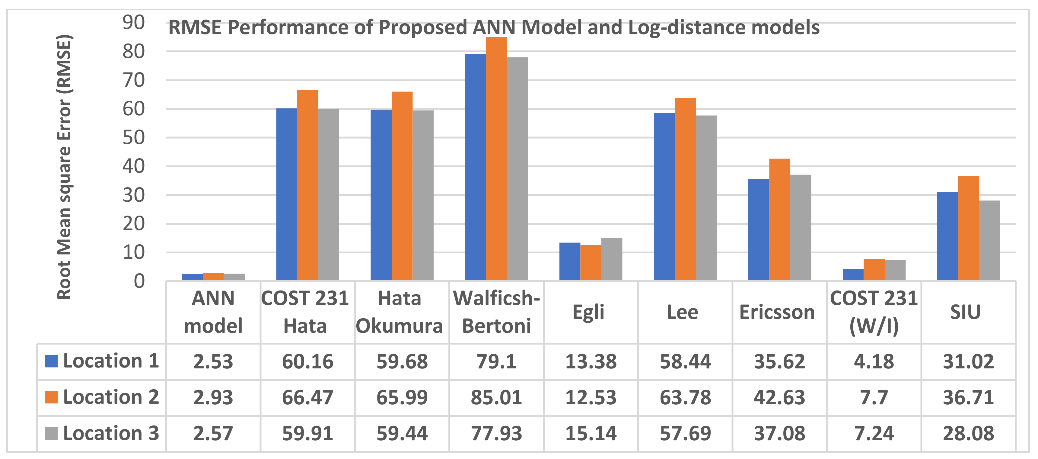
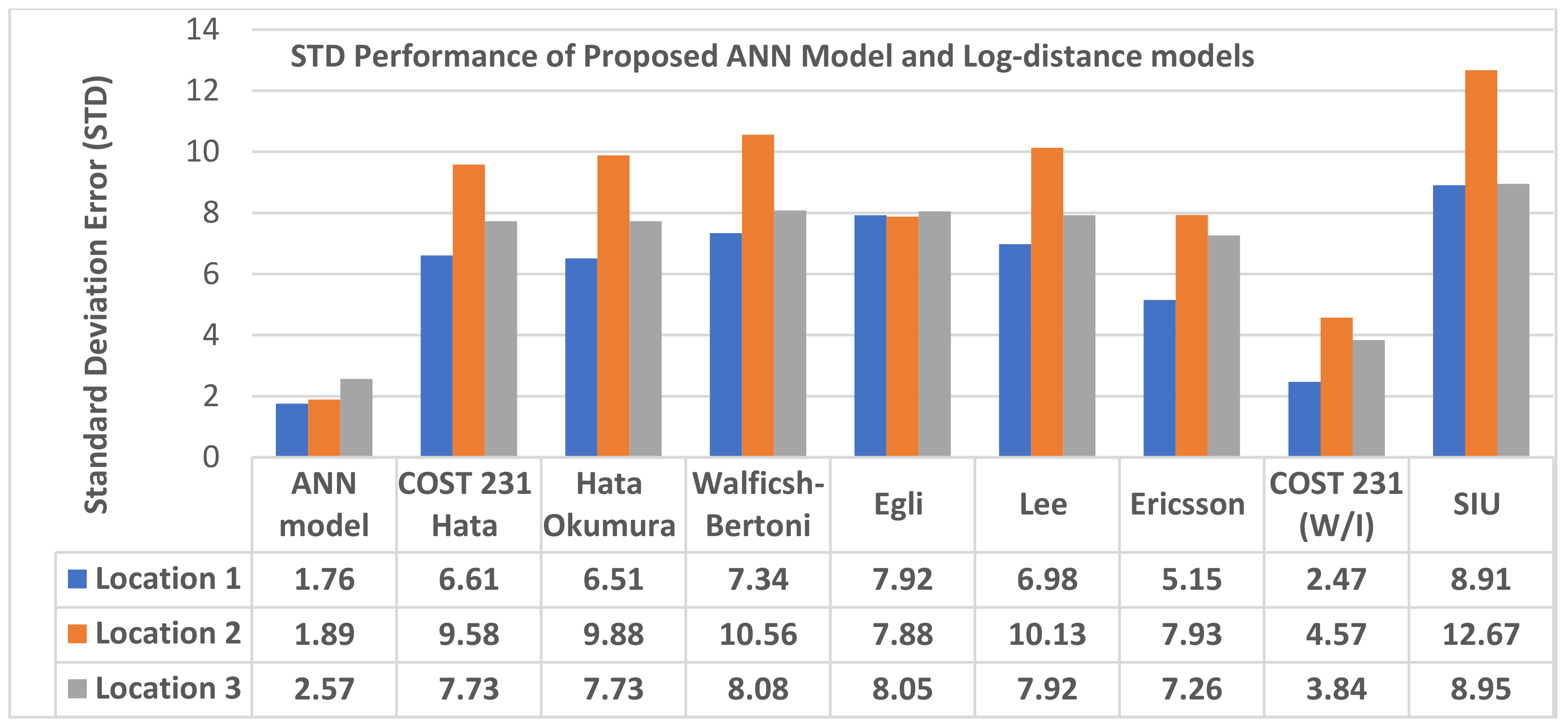
4.6. Comparison of Prediction Accuracy of Proposed Neural Network Model with Log-Distance Models

Detailed prediction capabilities of all the log-distance models and the proposed model on measured path loss data are provided in the plotted graphs of Figure 21, Figure 22 and Figure 23 in terms of MAE, RMSE and STD. The graphs show that the neural network model achieved the best predictions with marginal errors. The COST 213 (W/I) made the closest prediction to measured loss, but in terms of accuracy, the proposed neural network model achieved the best performance by 20%, 15% and 25%, respectively, across study sites. For example, while COST 213 (W/I) reached 3.34, 2.35 and 4.23 dB in terms of RMSE, the proposed neural network model attained 1.73, 2.11 and 1.45 dB across study sites. Generally, models which predict the path loss in the tested areas with RMSEs higher than the acceptable range of up to 6 dB are not selected as most suitable. However, such models could be further optimized for improved performance. The lower the RMSE value towards zero, the better the model. Regarding standard deviation error, COST 213 (W/I) achieved 1.73, 2.11 and 1.45 dB, while the proposed neural network model achieved 1.73, 2.11 and 1.45 dB, respectively. The poor predictions made by the log-distance-based models can be ascribed to due to dissimilarities and variations in environmental formations (hilly, mountainous or quasi-plain), weather conditions, soil electrical properties and terrain types that exist in different radio propagation environments.

5. Conclusions

The growing demand for mobile and fixed cellular telecommunication services have given substantial weight to the limited available radio frequency spectrum. Proper modelling and precise signal coverage predictions are crucial to utilizing this scarce resource effectively. Reliable predictive modeling of signal path loss aids in controlling the load on base station transmitters and assists in designing efficient radio network channels with less interference and coverage hole problems. The conventional log-distance-based statistical models for path loss prediction comprising the clustering factor, COST 234 Hata, free space, Hata, Lee models, etc., are generally limited for predicting signal attenuation losses, especially when employed in different environments other than the environment for which they have been designed.

The main objective of this paper was to develop a distinctive MLP-based path loss model with well-structured implementation network architecture, empowered with the grid search-based hyperparameter tuning method for optimal path loss approximation between mobile-station and base-station path lengths. The degree of prediction accuracy with the developed MLP network model over eight conventional log-distance-based path loss models is also clearly provided using first-order statistics. In summary, this research paper has revealed that:

• MLPANN-based path loss model with well-structured implementation network architecture, empowered with the right hyperparameter tuning algorithm is better than the standard long-distance path loss models
• the choice of both MLP-ANN modelling structure and selection of training algorithms do have a clear impact on the quality of its prediction proficiency. Specifically, in terms of MAE, RMSE and STD statistical values, the proposed model yielded up to 50% performance prediction accuracies improvement over the standard models on the acquired LTE path loss datasets.
• The selection of adaptive learning tuning hyperparameters of MLP-ANN and the tuning algorithm both have an impact on its overall predictive modelling capacity.

Future work would consider more hyperparameter selection techniques to optimize MLP model prediction accuracy during NN training. We also intend to explore more super layered training capacity of deep neural networks such as the long-short memory (LSTM) network model for predictive modelling of path loss data in our work.

References

1. Molisch, A.F. Wireless Communications, 2nd ed.; John Wiley & Sons, Inc.: Hoboken, NJ, USA, 2012; ISBN 9780470741870. [Google Scholar]
2. Goldsmith, A.J. Wireless Communications; Cambridge University Press: Cambridge, UK, 2005. [Google Scholar]
3. Isabona, J.; Imoize, A.L.; Ojo, S.; Lee, C.-C.; Li, C.-T. Atmospheric Propagation Modelling for Terrestrial Radio Frequency Communication Links in a Tropical Wet and Dry Savanna Climate. Information 2022, 13, 141. [Google Scholar] [CrossRef]
4. Isabona, J.; Konyeha, C.C.; Chinule, C.B.; Isaiah, G.P. Radio field strength propagation data and pathloss calculation methods in UMTS network. Adv. Phys. Theor. Appl. 2013, 21, 54–68. [Google Scholar]
5. Nawrocki, M.; Aghvami, H.; Dohler, M. Understanding UMTS Radio Network Modelling, Planning and Automated Optimisation: Theory and Practice; John Wiley & Sons: Hoboken, NJ, USA, 2006. [Google Scholar]
6. Nawrocki, M.J.; Dohler, M.; Aghvami, A.H. Modern approaches to radio network modelling and planning. In Understanding UMTS Radio Network Modelling, Planning and Automated Optimisation: Theory and Practice; John Wiley & Sons: Hoboken, NJ, USA, 2006; p. 3. [Google Scholar]
7. Sharma, P.K.; Singh, R.K. Comparative analysis of propagation path loss models with field measured data. Int. J. Eng. Sci. Technol. 2010, 2, 2008–2013. [Google Scholar]
8. Ajose, S.O.; Imoize, A.L. Propagation measurements and modelling at 1800 MHz in Lagos Nigeria. Int. J. Wirel. Mob. Comput. 2013, 6, 165–174. [Google Scholar] [CrossRef]
9. Ojo, S.; Imoize, A.; Alienyi, D. Radial basis function neural network path loss prediction model for LTE networks in multitransmitter signal propagation environments. Int. J. Commun. Syst. 2021, 34, e4680. [Google Scholar] [CrossRef]
10. Imoize, A.L.; Ibhaze, A.E.; Nwosu, P.O.; Ajose, S.O. Determination of Best-fit Propagation Models for Pathloss Prediction of a 4G LTE Network in Suburban and Urban Areas of Lagos, Nigeria. West Indian J. Eng. 2019, 41, 13–21. [Google Scholar]
11. Ibhaze, A.E.; Imoize, A.L.; Ajose, S.O.; John, S.N.; Ndujiuba, C.U.; Idachaba, F.E. An Empirical Propagation Model for Path Loss Prediction at 2100 MHz in a Dense Urban Environment. Indian J. Sci. Technol. 2017, 10, 1–9. [Google Scholar] [CrossRef]
12. Rathore, M.M.; Paul, A.; Rho, S.; Khan, M.; Vimal, S.; Shah, S.A. Smart traffic control: Identifying driving-violations using fog devices with vehicular cameras in smart cities. Sustain. Cities Soc. 2021, 71, 102986. [Google Scholar] [CrossRef]
13. Imoize, A.L.; Tofade, S.O.; Ughegbe, G.U.; Anyasi, F.I.; Isabona, J. Updating analysis of key performance indicators of 4G LTE network with the prediction of missing values of critical network parameters based on experimental data from a dense urban environment. Data Br. 2022, 42, 108240. [Google Scholar] [CrossRef]
14. Fujimoto, K. Mobile Antenna Systems Handbook; Artech House: Norwood, MA, USA, 2008; ISBN 1596931272. [Google Scholar]
15. Tataria, H.; Haneda, K.; Molisch, A.F.; Shafi, M.; Tufvesson, F. Standardization of Propagation Models for Terrestrial Cellular Systems: A Historical Perspective. Int. J. Wirel. Inf. Networks 2021, 28, 20–44. [Google Scholar] [CrossRef]
16. Hanci, B.Y.; Cavdar, I.H. Mobile radio propagation measurements and tuning the path loss model in urban areas at GSM-900 band in Istanbul-Turkey. In Proceedings of the IEEE 60th Vehicular Technology Conference, 2004, VTC2004-Fall, Los Angeles, CA, USA, 26–29 September 2004; Volume 1, pp. 139–143. [Google Scholar]
17. Ekpenyong, M.; Isabona, J.; Ekong, E. On Propagation Path Loss Models For 3-G Based Wireless Networks: A Comparative Analysis. Comput. Sci. Telecommun. 2010, 25, 74–84. [Google Scholar]
18. Isabona, J. Wavelet Generalized Regression Neural Network Approach for Robust Field Strength Prediction. Wirel. Pers. Commun. 2020, 114, 3635–3653. [Google Scholar] [CrossRef]
19. Imoize, A.L.; Oseni, A.I. Investigation and pathloss modeling of fourth generation long term evolution network along major highways in Lagos Nigeria. Ife J. Sci. 2019, 21, 39–60. [Google Scholar] [CrossRef]
20. Imoize, A.L.; Ogunfuwa, T.E. Propagation measurements of a 4G LTE network in Lagoon environment. Niger. J. Technol. Dev. 2019, 16, 1–9. [Google Scholar] [CrossRef] [Green Version]
21. Imoize, A.L.; Dosunmu, A.I. Path Loss Characterization of Long Term Evolution Network for. Jordan J. Electr. Eng. 2018, 4, 114–128. [Google Scholar]
22. Ekpenyong, M.E.; Robinson, S.; Isabona, J. Macrocellular propagation prediction for wireless communications in urban environments. J. Comput. Sci. Technol. 2010, 10, 130–136. [Google Scholar]
23. Nadir, Z. Empirical pathloss characterization for Oman. In Proceedings of the 2012 Computing, Communications and Applications Conference, Tamilnadu, India, 22–24 February 2012; pp. 133–137. [Google Scholar] [CrossRef]
24. Hunter, D.; Yu, H.; Pukish III, M.S.; Kolbusz, J.; Wilamowski, B.M. Selection of proper neural network sizes and architectures—A comparative study. IEEE Trans. Ind. Informatics 2012, 8, 228–240. [Google Scholar] [CrossRef]
25. Imoize, A.L.; Ibhaze, A.E.; Atayero, A.A.; Kavitha, K.V.N. Standard Propagation Channel Models for MIMO Communication Systems. Wirel. Commun. Mob. Comput. 2021, 2021, 8838792. [Google Scholar] [CrossRef]
26. Khan, N.; Haq, I.U.; Khan, S.U.; Rho, S.; Lee, M.Y.; Baik, S.W. DB-Net: A novel dilated CNN based multi-step forecasting model for power consumption in integrated local energy systems. Int. J. Electr. Power Energy Syst. 2021, 133, 107023. [Google Scholar] [CrossRef]
27. Jo, H.-S.; Park, C.; Lee, E.; Choi, H.K.; Park, J. Path loss prediction based on machine learning techniques: Principal component analysis, artificial neural network, and Gaussian process. Sensors 2020, 20, 1927. [Google Scholar] [CrossRef] [Green Version]
28. Guo, D.; Zhang, Y.; Xiang, Q.; Li, Z. Improved radio frequency identification indoor localization method via radial basis function neural network. Math. Probl. Eng. 2014, 2014, 420482. [Google Scholar] [CrossRef] [Green Version]
29. Guo, Y.; Liu, Y.; Li, S. Modeling and Simulation of Terahertz Indoor Wireless Channel Based on Radial Basis Function Neural Network. In Proceedings of the 2021 International Conference on Microwave and Millimeter Wave Technology (ICMMT), Nanjing, China, 23–26 May 2021; pp. 1–3. [Google Scholar]
30. Annepu, V.; Rajesh, A.; Bagadi, K. Radial basis function-based node localization for unmanned aerial vehicle-assisted 5G wireless sensor networks. Neural Comput. Appl. 2021, 33, 12333–12346. [Google Scholar] [CrossRef]
31. Huang, G.-B. Learning capability and storage capacity of two-hidden-layer feedforward networks. IEEE Trans. Neural Netw. 2003, 14, 274–281. [Google Scholar] [CrossRef] [Green Version]
32. Abhayawardhana, V.S.; Wassellt, I.J.; Crosby, D.; Sellars, M.P.; Brown, M.G. Comparison of empirical propagation path loss models for fixed wireless access systems. In Proceedings of the IEEE Vehicular Technology Conference, Stockholm, Sweden, 30 May–1 June 2005; Volume 61, pp. 73–77. [Google Scholar]
33. Hinga, S.K.; Atayero, A.A. Deterministic 5G mmWave Large-Scale 3D Path Loss Model for Lagos Island, Nigeria. IEEE Access 2021, 9, 134270–134288. [Google Scholar] [CrossRef]
34. Haykin, S. Neural networks: A guided tour. Soft Comput. Intell. Syst. theory Appl. 1999, 71, 71–80. [Google Scholar]
35. Isabona, J.; Osaigbovo, A.I. Investigating predictive capabilities of RBFNN, MLPNN and GRNN models for LTE cellular network radio signal power datasets. FUOYE J. Eng. Technol. 2019, 4, 155–159. [Google Scholar] [CrossRef]
36. Sotiroudis, S.P.; Goudos, S.K.; Gotsis, K.A.; Siakavara, K.; Sahalos, J.N. Modeling by optimal artificial neural networks the prediction of propagation path loss in urban environments. In Proceedings of the 2013 IEEE-APS Topical Conference on Antennas and Propagation in Wireless Communications (APWC), Turin, Italy, 9–13 September 2013; pp. 599–602. [Google Scholar]
37. Isabona, J.; Imoize, A.L. Terrain-based adaption of propagation model loss parameters using non-linear square regression. J. Eng. Appl. Sci. 2021, 68, 33. [Google Scholar] [CrossRef]
38. Phillips, C.; Sicker, D.; Grunwald, D. A Survey of Wireless Path Loss Prediction and Coverage Mapping Methods. IEEE Commun. Surv. Tutorials 2013, 15, 255–270. [Google Scholar] [CrossRef]
39. Imoize, A.L.; Oyedare, T.; Ezekafor, C.G.; Shetty, S. Deployment of an Energy Efficient Routing Protocol for Wireless Sensor Networks Operating in a Resource Constrained Environment. Trans. Networks Commun. 2019, 7, 34–50. [Google Scholar] [CrossRef] [Green Version]
40. Imoize, A.L.; Ajibola, O.A.; Oyedare, T.R.; Ogbebor, J.O.; Ajose, S.O. Development of an Energy-Efficient Wireless Sensor Network Model for Perimeter Surveillance. Int. J. Electr. Eng. Appl. Sci. 2021, 4, 1–17. [Google Scholar]
41. Imoize, A.L. Analysis of Propagation Models for Mobile Radio Reception at 1800MHz. Master’s Thesis, University of Lagos, Lagos, Nigeria, 2011. [Google Scholar]
42. Isabona, J.; Ojuh, D. Adaptation of Propagation Model Parameters toward Efficient Cellular Network Planning using Robust LAD Algorithm. Int. J. Wirel. Microw. Technol. 2020, 10, 13–24. [Google Scholar] [CrossRef]
43. Imoize, A.L.; Orolu, K.; Atayero, A.A.-A. Analysis of key performance indicators of a 4G LTE network based on experimental data obtained from a densely populated smart city. Data Br. 2020, 29, 105304. [Google Scholar] [CrossRef] [PubMed]
44. Ojo, S.; Akkaya, M.; Sopuru, J.C. An ensemble machine learning approach for enhanced path loss predictions for 4G LTE wireless networks. Int. J. Commun. Syst. 2022, 35, e5101. [Google Scholar] [CrossRef]
45. Ebhota, V.C.; Isabona, J.; Srivastava, V.M. Improved adaptive signal power loss prediction using combined vector statistics based smoothing and neural network approach. Prog. Electromagn. Res. C 2018, 82, 155–169. [Google Scholar] [CrossRef] [Green Version]
46. Ebhota, V.C.; Isabona, J.; Srivastava, V.M. Base line knowledge on propagation modelling and prediction techniques in wireless communication networks. J. Eng. Appl. Sci. 2018, 13, 1919–1934. [Google Scholar]
47. Coskun, N.; Yildirim, T. The effects of training algorithms in MLP network on image classification. In Proceedings of the International Joint Conference on Neural Networks, Portland, OR, USA, 20–24 July 2003; Volume 2, pp. 1223–1226. [Google Scholar]
48. Salman, M.A.; Popoola, S.I.; Faruk, N.; Surajudeen-Bakinde, N.T.; Oloyede, A.A.; Olawoyin, L.A. Adaptive Neuro-Fuzzy model for path loss prediction in the VHF band. In Proceedings of the 2017 International Conference on Computing Networking and Informatics (ICCNI), Lagos, Nigeria, 29–31 October 2017; pp. 1–6. [Google Scholar]
49. Aldossari, S.; Chen, K.-C. Predicting the path loss of wireless channel models using machine learning techniques in mmwave urban communications. In Proceedings of the 2019 22nd International Symposium on Wireless Personal Multimedia Communications (WPMC), Lisbon, Portugal, 24–27 November 2019; pp. 1–6. [Google Scholar]
50. Ahmadien, O.; Ates, H.F.; Baykas, T.; Gunturk, B.K. Predicting Path Loss Distribution of an Area From Satellite Images Using Deep Learning. IEEE Access 2020, 8, 64982–64991. [Google Scholar] [CrossRef]
51. Turan, B.; Coleri, S. Machine learning based channel modeling for vehicular visible light communication. IEEE Trans. Veh. Technol. 2021, 70, 9659–9672. [Google Scholar] [CrossRef]
52. Ates, H.F.; Hashir, S.M.; Baykas, T.; Gunturk, B.K. Path loss exponent and shadowing factor prediction from satellite images using deep learning. IEEE Access 2019, 7, 101366–101375. [Google Scholar] [CrossRef]
53. Huang, J.; Cao, Y.; Raimundo, X.; Cheema, A.; Salous, S. Rain statistics investigation and rain attenuation modeling for millimeter wave short-range fixed links. IEEE Access 2019, 7, 156110–156120. [Google Scholar] [CrossRef]
54. Zhang, Y.; Wen, J.; Yang, G.; He, Z.; Wang, J. Path loss prediction based on machine learning: Principle, method, and data expansion. Appl. Sci. 2019, 9, 1908. [Google Scholar] [CrossRef] [Green Version]
55. Nguyen, D.C.; Cheng, P.; Ding, M.; Lopez-Perez, D.; Pathirana, P.N.; Li, J.; Seneviratne, A.; Li, Y.; Poor, H.V. Enabling AI in future wireless networks: A data life cycle perspective. IEEE Commun. Surv. Tutor. 2020, 23, 553–595. [Google Scholar] [CrossRef]
56. Ferreira, G.P.; Matos, L.J.; Silva, J.M.M. Improvement of outdoor signal strength prediction in UHF band by artificial neural network. IEEE Trans. Antennas Propag. 2016, 64, 5404–5410. [Google Scholar] [CrossRef]
57. Singh, H.; Gupta, S.; Dhawan, C.; Mishra, A. Path loss prediction in smart campus environment: Machine learning-based approaches. In Proceedings of the 2020 IEEE 91st Vehicular Technology Conference (VTC2020-Spring), Antwerp, Belgium, 25–28 May 2020; pp. 1–5. [Google Scholar]
58. Thrane, J.; Zibar, D.; Christiansen, H.L. Model-aided deep learning method for path loss prediction in mobile communication systems at 2.6 GHz. IEEE Access 2020, 8, 7925–7936. [Google Scholar] [CrossRef]
59. Shrestha, A.; Mahmood, A. Review of deep learning algorithms and architectures. IEEE Access 2019, 7, 53040–53065. [Google Scholar] [CrossRef]
60. Nguyen, C.; Cheema, A.A. A deep neural network-based multi-frequency path loss prediction model from 0.8 GHz to 70 GHz. Sensors 2021, 21, 5100. [Google Scholar] [CrossRef]
61. Challita, U.; Dong, L.; Saad, W. Deep learning for proactive resource allocation in LTE-U networks. In Proceedings of the European Wireless Technology Conference, Dresden, Germany, 15 May 2017. [Google Scholar]
62. Song, W.; Zeng, F.; Hu, J.; Wang, Z.; Mao, X. An unsupervised-learning-based method for multi-hop wireless broadcast relay selection in urban vehicular networks. In Proceedings of the 2017 IEEE 85th Vehicular Technology Conference (VTC Spring), Sydney, NSW, Australia, 4–7 June 2017; pp. 1–5. [Google Scholar]
63. Ebhota, V.C.; Isabona, J.; Srivastava, V.M. Environment-Adaptation Based Hybrid Neural Network Predictor for Signal Propagation Loss Prediction in Cluttered and Open Urban Microcells. Wirel. Pers. Commun. 2019, 104, 935–948. [Google Scholar] [CrossRef]
64. Isabona, J.; Babalola, M. Statistical Tuning of Walfisch-Bertoni Pathloss Model based on Building and Street Geometry Parameters in Built-up Terrains. Am. J. Phys. Appl. 2013, 1, 10–16. [Google Scholar]
65. Bird, J. Engineering Mathematics, 5th ed.; Newness: Los Angeles, CA, USA, 2010; ISBN 9780750681520. [Google Scholar]
Figure 1. Illustration of the TEMS Drive Test Measurement System.
Applsci 12 05713 g001
Figure 2. Scheme of a three-layered ANN multi-layer perceptron.
Applsci 12 05713 g002
Figure 3. ANN MLP Model Structure for Path Loss Prediction.
Applsci 12 05713 g003
Figure 4. Flowchart for the execution of Proposed Predictive Modelling with MLP Neural Network.
Applsci 12 05713 g004
Figure 5. Overall Performance Error Statistics with MAE, STD and RMSE.
Applsci 12 05713 g005
Figure 6. Overall Performance Error Statistics with R (%) and COE (%).
Applsci 12 05713 g006
Figure 7. Standard deviation (STD) statistics with one, two and three layers of training.
Applsci 12 05713 g007
Figure 8. Root Mean Error performance statistics with one, two and three layers of training.
Applsci 12 05713 g008
Figure 9. Comparison between measured loss and the prediction ANN model in site 1.
Applsci 12 05713 g009
Figure 10. Comparison between measured loss and the prediction ANN model in site 2.
Applsci 12 05713 g010
Figure 11. Comparison between measured loss and the prediction ANN model in site 3.
Applsci 12 05713 g011
Figure 12. Prediction performance with correlation coefficient in site 1.
Applsci 12 05713 g012
Figure 13. Prediction performance with correlation coefficient in site 2.
Applsci 12 05713 g013
Figure 14. Prediction performance with correlation coefficient in site 3.
Applsci 12 05713 g014
Figure 15. Network training cycles in site 1.
Applsci 12 05713 g015
Figure 16. Network training cycles in site 2.
Applsci 12 05713 g016
Figure 17. Network training cycles in site 3.
Applsci 12 05713 g017
Figure 18. Mean prediction error statistics along with Data points in site 1.
Applsci 12 05713 g018
Figure 19. Mean prediction error statistics along with Data points in site 2.
Applsci 12 05713 g019
Figure 20. Mean prediction error statistics along with Data points in site 3.
Applsci 12 05713 g020
Figure 21. A comparison of mean absolute error statistics between the proposed ANN model and log-distance models on measured path loss in site locations 1, 2 and 3.
Applsci 12 05713 g021
Figure 22. A comparison of root mean absolute error statistics between the proposed ANN model and log-distance models on measured path loss in site locations 1, 2 and 3.
Applsci 12 05713 g022
Figure 23. A comparison of standard deviation error statistics between the proposed ANN and log-distance models on measured path loss in site locations 1, 2 and 3.
Applsci 12 05713 g023