
Cycle Mutation: Evolving Permutations via Cycle Induction


Abstract
1. Introduction
2. Background
2.1. Permutation Mutation Operators
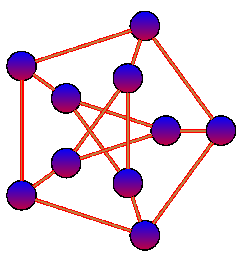
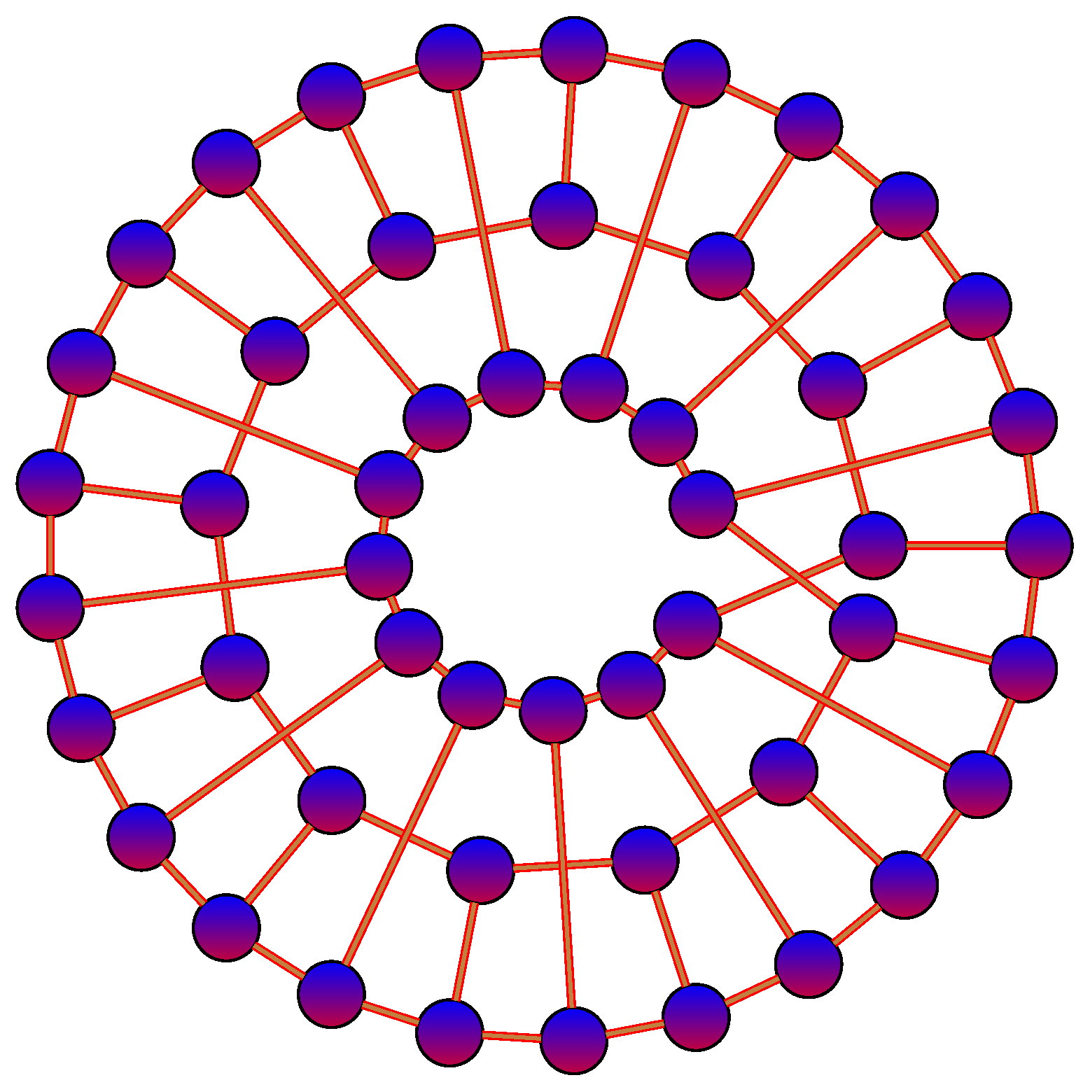
2.2. Permutation Cycles
2.3. Cycle Crossover (CX)
2.4. Test Problems
2.4.1. TSP
2.4.2. QAP
2.4.3. LCS
3. Methods
3.1. Cycle Mutation
3.1.1. Shared Notation and Operations
| Algorithm 1 |
|
| Algorithm 2 |
|
| Algorithm 3 |
|
3.1.2.
| Algorithm 4 |
|
3.1.3.
| Algorithm 5 |
|
3.1.4. Asymptotic Runtime Summary
3.2. New Measures of Permutation Distance
3.2.1. Cycle Distance
3.2.2. Cycle Edit Distance
3.2.3. K-Cycle Distance
3.3. Fitness Landscape Analysis
3.3.1. Fitness Landscape Diameter
3.3.2. Fitness Distance Correlation
3.3.3. Search Landscape Calculus
3.3.4. Summary of Fitness Landscape Analysis Findings
4. Results
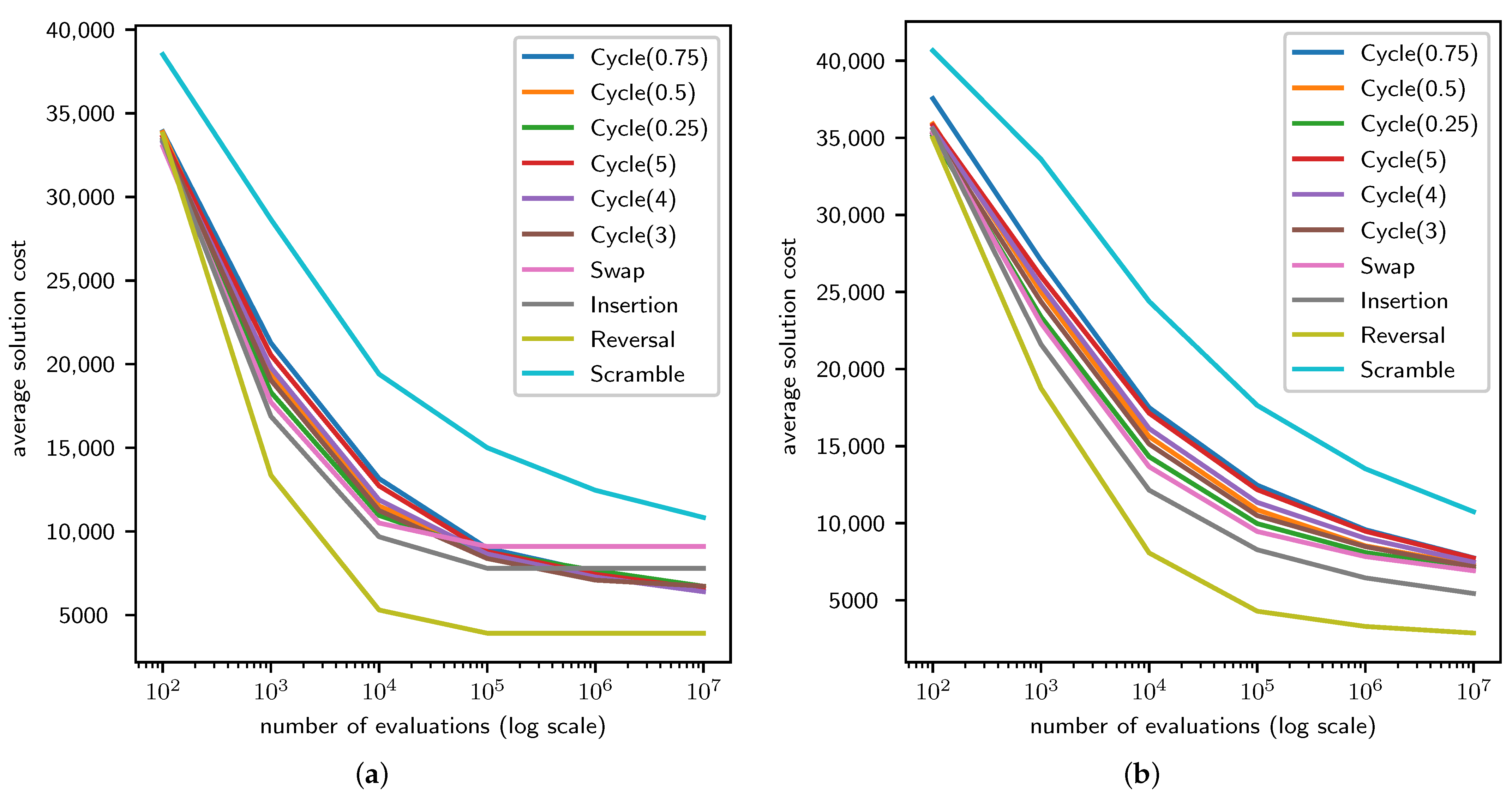
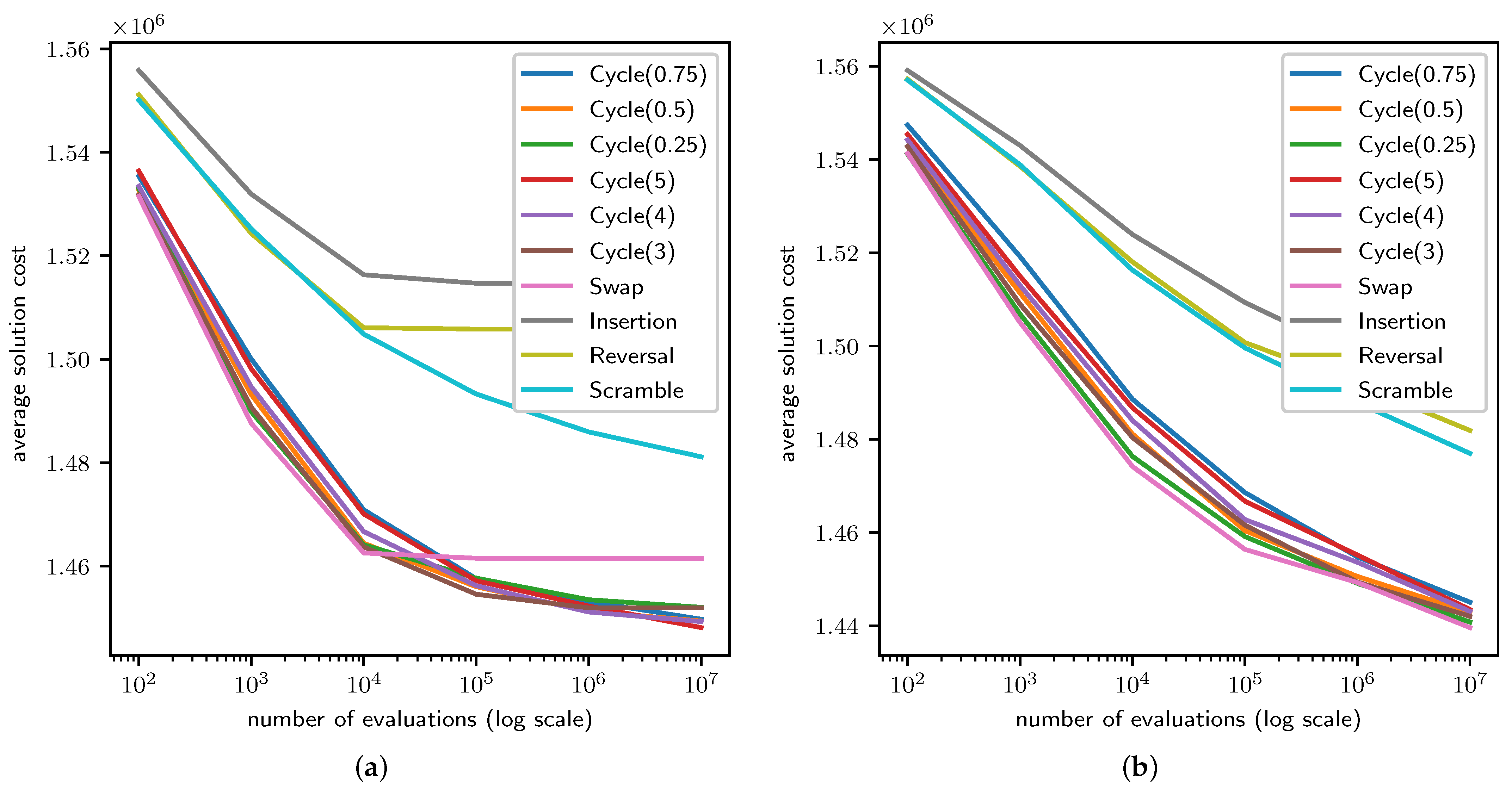
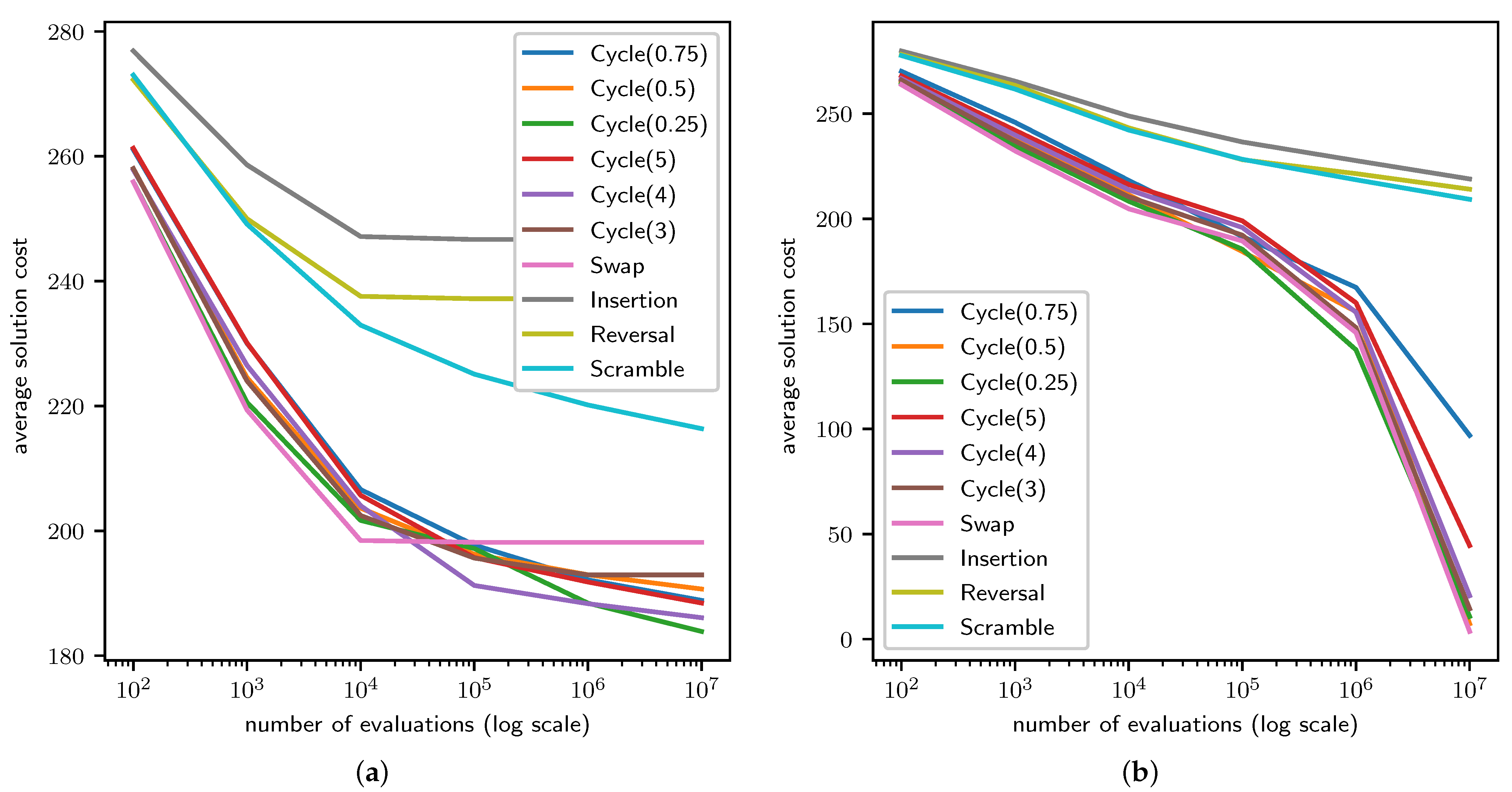
4.1. TSP Results
4.2. QAP Results
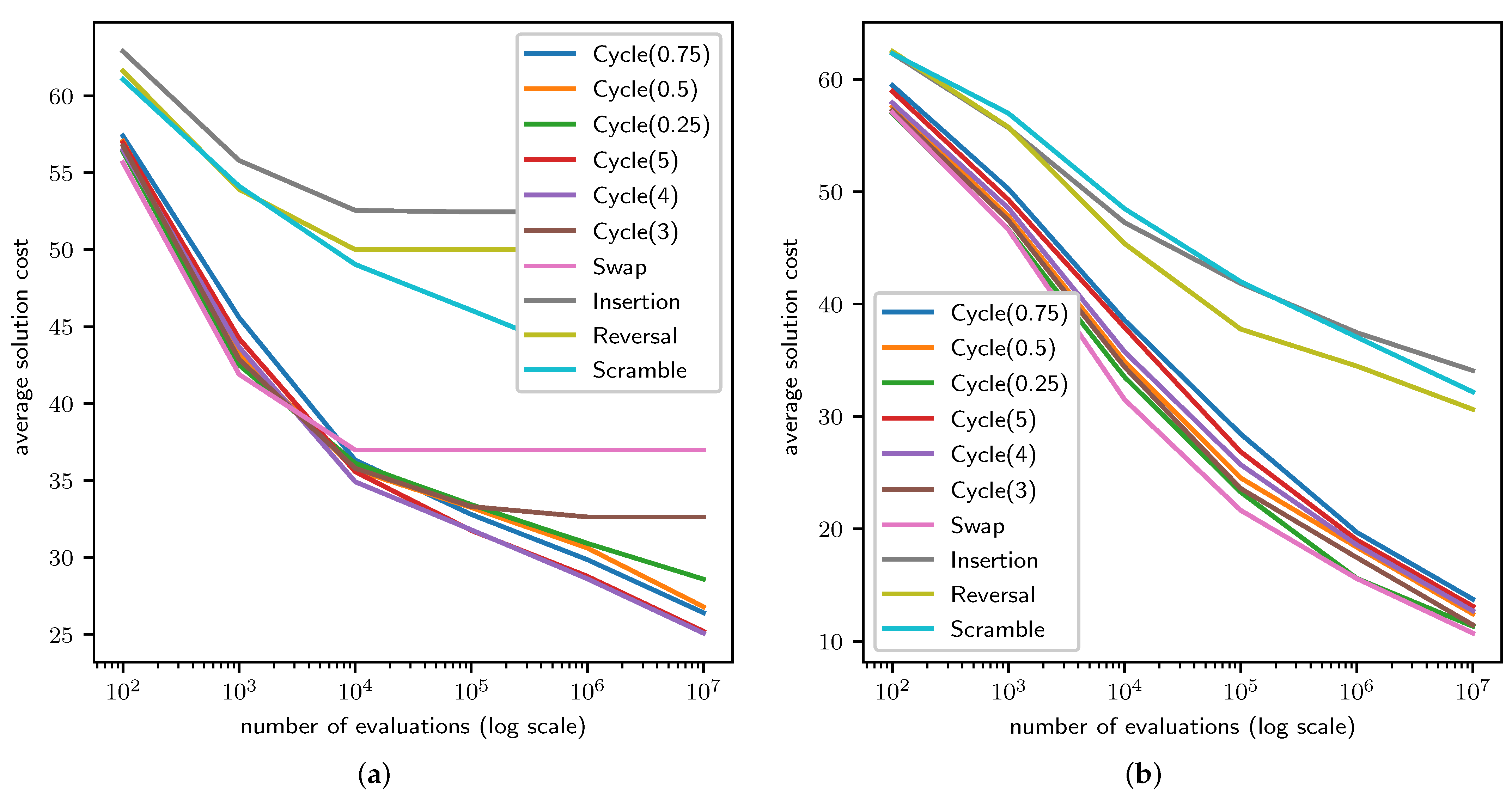
4.3. LCS Results
5. Discussion and Conclusions
Funding
Institutional Review Board Statement
Informed Consent Statement
Data Availability Statement
Conflicts of Interest
Abbreviations
| CX | Cycle crossover |
| EA | Evolutionary algorithm |
| ES | Evolution strategies |
| FDC | Fitness distance correlation |
| GA | Genetic algorithm |
| LCS | Largest common subgraph |
| QAP | Quadratic assignment problem |
| SA | Simulated annealing |
| TSP | Traveling salesperson problem |
References
- Mitchell, M. An Introduction to Genetic Algorithms; MIT Press: Cambridge, MA, USA, 1998. [Google Scholar]
- Beyer, H. The Theory of Evolution Strategies; Natural Computing Series; Springer: Berlin/Heidelberg, Germany, 2013. [Google Scholar]
- Langdon, W.; Poli, R. Foundations of Genetic Programming; Springer: Berlin/Heidelberg, Germany, 2013. [Google Scholar]
- Cuéllar, M.; Gómez-Torrecillas, J.; Lobillo, F.; Navarro, G. Genetic algorithms with permutation-based representation for computing the distance of linear codes. Swarm Evol. Comput. 2021, 60, 100797. [Google Scholar] [CrossRef]
- Koohestani, B. A crossover operator for improving the efficiency of permutation-based genetic algorithms. Expert Syst. Appl. 2020, 151, 113381. [Google Scholar] [CrossRef]
- Shabash, B.; Wiese, K.C. PEvoSAT: A Novel Permutation Based Genetic Algorithm for Solving the Boolean Satisfiability Problem. In Proceedings of the 15th Annual Conference on Genetic and Evolutionary Computation, Amsterdam, The Netherlands, 6–10 July 2013; Association for Computing Machinery: New York, NY, USA, 2013; pp. 861–868. [Google Scholar] [CrossRef]
- Kalita, Z.; Datta, D.; Palubeckis, G. Bi-objective corridor allocation problem using a permutation-based genetic algorithm hybridized with a local search technique. Soft Comput. 2019, 23, 961–986. [Google Scholar] [CrossRef]
- Shakya, S.; Lee, B.S.; Di Cairano-Gilfedder, C.; Owusu, G. Spares parts optimization for legacy telecom networks using a permutation-based evolutionary algorithm. In Proceedings of the IEEE Congress on Evolutionary Computation (CEC), Donostia, Spain, 5–8 June 2017; pp. 1742–1748. [Google Scholar] [CrossRef]
- Mironovich, V.; Buzdalov, M.; Vyatkin, V. Evaluation of Permutation-Based Mutation Operators on the Problem of Automatic Connection Matching in Closed-Loop Control System. In Recent Advances in Soft Computing and Cybernetics; Matoušek, R., Kůdela, J., Eds.; Springer International Publishing: Berlin/Heidelberg, Germany, 2021; pp. 41–51. [Google Scholar] [CrossRef]
- Hinterding, R. Gaussian mutation and self-adaption for numeric genetic algorithms. In Proceedings of the IEEE International Conference on Evolutionary Computation, Perth, WA, Australia, 29 November–1 December 1995; Volume 1, pp. 384–389. [Google Scholar] [CrossRef]
- Szu, H.; Hartley, R. Nonconvex optimization by fast simulated annealing. Proc. IEEE 1987, 75, 1538–1540. [Google Scholar] [CrossRef]
- Campos, V.; Laguna, M.; Marti, R. Context-Independent Scatter and Tabu Search for Permutation Problems. INFORMS J. Comput. 2005, 17, 111–122. [Google Scholar] [CrossRef][Green Version]
- Cicirello, V.A. Classification of Permutation Distance Metrics for Fitness Landscape Analysis. In Proceedings of the 11th International Conference on Bio-Inspired Information and Communication Technologies, Pittsburgh, PA, USA, 13–14 March 2019; Springer: New York, NY, USA, 2019; pp. 81–97. [Google Scholar] [CrossRef]
- Garey, M.R.; Johnson, D.S. Computers and Intractability: A Guide to the Theory of NP-Completeness; W. H. Freeman & Co.: New York, NY, USA, 1979. [Google Scholar]
- Eiben, A.E.; Smith, J.E. Introduction to Evolutionary Computing, 2nd ed.; Springer: Berlin/Heidelberg, Germany, 2015. [Google Scholar]
- Davis, L. Applying Adaptive Algorithms to Epistatic Domains. In Proceedings of the International Joint Conference on Artificial Intelligence, San Francisco, CA, USA, 18–23 August 1985; pp. 162–164. [Google Scholar]
- Cicirello, V.A. Non-Wrapping Order Crossover: An Order Preserving Crossover Operator that Respects Absolute Position. In Proceedings of the Genetic and Evolutionary Computation Conference, Seattle, WA, USA, 8–12 July 2006; ACM Press: New York, NY, USA, 2006; Volume 2, pp. 1125–1131. [Google Scholar] [CrossRef]
- Syswerda, G. Schedule Optimization using Genetic Algorithms. In Handbook of Genetic Algorithms; Davis, L., Ed.; Van Nostrand Reinhold: New York, NY, USA, 1991. [Google Scholar]
- Goldberg, D.E.; Lingle, R. Alleles, Loci, and the Traveling Salesman Problem. In Proceedings of the 1st International Conference on Genetic Algorithms, Sheffield, UK, 12–14 September 1995; Lawrence Erlbaum Associates, Inc.: Mahwah, NJ, USA, 1985; pp. 154–159. [Google Scholar]
- Cicirello, V.A.; Smith, S.F. Modeling GA Performance for Control Parameter Optimization. In Proceedings of the Genetic and Evolutionary Computation Conference; Morgan Kaufmann Publishers: San Francisco, CA, USA, 2000; pp. 235–242. [Google Scholar]
- Bierwirth, C.; Mattfeld, D.; Kopfer, H. On permutation representations for scheduling problems. In Proceedings of the International Conference on Parallel Problem Solving from Nature; Springer: Berlin/Heidelberg, Germany, 1996; pp. 310–318. [Google Scholar]
- Nagata, Y.; Kobayashi, S. Edge Assembly Crossover: A High-Power Genetic Algorithm for the Travelling Salesman Problem. In Proceedings of the International Conference on Genetic Algorithms, East Lansing, MI, USA, 19–23 July 1997; pp. 450–457. [Google Scholar]
- Watson, J.P.; Ross, C.; Eisele, V.; Denton, J.; Bins, J.; Guerra, C.; Whitley, L.D.; Howe, A.E. The Traveling Salesrep Problem, Edge Assembly Crossover, and 2-opt. In Proceedings of the International Conference on Parallel Problem Solving from Nature, Amsterdam, The Netherlands, 27–30 September 1998; Springer: Berlin/Heidelberg, Germany, 1998; pp. 823–834. [Google Scholar]
- Oliver, I.M.; Smith, D.J.; Holland, J.R.C. A study of permutation crossover operators on the traveling salesman problem. In Proceedings of the 2nd International Conference on Genetic Algorithms, Cambridge, MA, USA, 1 July 1987; Lawrence Erlbaum Associates, Inc.: Mahwah, NJ, USA, 1987; pp. 224–230. [Google Scholar]
- Delahaye, D.; Chaimatanan, S.; Mongeau, M. Simulated Annealing: From Basics to Applications. In Handbook of Metaheuristics; Gendreau, M., Potvin, J.Y., Eds.; Springer: Berlin/Heidelberg, Germany, 2019; pp. 1–35. [Google Scholar] [CrossRef]
- Laarhoven, P.J.M.; Aarts, E.H.L. Simulated Annealing: Theory and Applications; Kluwer Academic Publishers: Norwell, MA, USA, 1987. [Google Scholar]
- Kirkpatrick, S.; Gelatt, C.D.; Vecchi, M.P. Optimization by Simulated Annealing. Science 1983, 220, 671–680. [Google Scholar] [CrossRef]
- Jones, T.; Forrest, S. Fitness Distance Correlation as a Measure of Problem Difficulty for Genetic Algorithms. In Proceedings of the 6th International Conference on Genetic Algorithms, Pittsburgh, PA, USA, 15–19 July 1995; Morgan Kaufmann: San Francisco, CA, USA, 1995; pp. 184–192. [Google Scholar]
- National Academies of Sciences, Engineering, and Medicine. Reproducibility and Replicability in Science; The National Academies Press: Washington, DC, USA, 2019. [Google Scholar] [CrossRef]
- Cicirello, V.A. Chips-n-Salsa: A Java Library of Customizable, Hybridizable, Iterative, Parallel, Stochastic, and Self-Adaptive Local Search Algorithms. J. Open Source Softw. 2020, 5, 2448. [Google Scholar] [CrossRef]
- Cicirello, V.A. JavaPermutationTools: A Java Library of Permutation Distance Metrics. J. Open Source Softw. 2018, 3, 950. [Google Scholar] [CrossRef]
- Cicirello, V.A. The Permutation in a Haystack Problem and the Calculus of Search Landscapes. IEEE Trans. Evol. Comput. 2016, 20, 434–446. [Google Scholar] [CrossRef]
- Knuth, D.E. The Art of Computer Programming, Volume 1, Fundamental Algorithms, 3rd ed.; Addison Wesley: Boston, MA, USA, 1997. [Google Scholar]
- Junior Mele, U.; Maria Gambardella, L.; Montemanni, R. Machine Learning Approaches for the Traveling Salesman Problem: A Survey. In Proceedings of the 8th International Conference on Industrial Engineering and Applications, Barcelona, Spain, 8–11 January 2021; ACM: New York, NY, USA, 2021; pp. 182–186. [Google Scholar] [CrossRef]
- Mele, U.J.; Chou, X.; Gambardella, L.M.; Montemanni, R. Reinforcement Learning and Additional Rewards for the Traveling Salesman Problem. In Proceedings of the 8th International Conference on Industrial Engineering and Applications, Barcelona, Spain, 8–11 January 2021; ACM: New York, NY, USA, 2021; pp. 198–204. [Google Scholar] [CrossRef]
- Wang, R.L.; Gao, S. A Co-Evolutionary Hybrid ACO for Solving Traveling Salesman Problem. In Proceedings of the 5th International Conference on Computer Science and Application Engineering, Virtual Conference, Sanya, China, 19–21 October 2021; ACM: New York, NY, USA, 2021; pp. 1–4. [Google Scholar]
- Dinh, Q.T.; Do, D.D.; Hà, M.H. Ants Can Solve the Parallel Drone Scheduling Traveling Salesman Problem. In Proceedings of the Genetic and Evolutionary Computation Conference, Lille, France, 10–14 July 2021; ACM: New York, NY, USA, 2021; pp. 14–21. [Google Scholar] [CrossRef]
- Varadarajan, S.; Whitley, D. A Parallel Ensemble Genetic Algorithm for the Traveling Salesman Problem. In Proceedings of the Genetic and Evolutionary Computation Conference, Lille, France, 10–14 July 2021; ACM: New York, NY, USA, 2021; pp. 636–643. [Google Scholar] [CrossRef]
- Nagata, Y. High-Order Entropy-Based Population Diversity Measures in the Traveling Salesman Problem. Evol. Comput. 2020, 28, 595–619. [Google Scholar] [CrossRef]
- Ibada, A.J.; Tuu-Szabo, B.; Koczy, L.T. A New Efficient Tour Construction Heuristic for the Traveling Salesman Problem. In Proceedings of the 5th International Conference on Intelligent Systems, Metaheuristics & Swarm Intelligence, Victoria, Seychelles, 10–11 April 2021; ACM: New York, NY, USA, 2021; pp. 71–76. [Google Scholar] [CrossRef]
- Dell’Amico, M.; Montemanni, R.; Novellani, S. A Random Restart Local Search Matheuristic for the Flying Sidekick Traveling Salesman Problem. In Proceedings of the 8th International Conference on Industrial Engineering and Applications, Barcelona, Spain, 8–11 January 2021; ACM: New York, NY, USA, 2021; pp. 205–209. [Google Scholar] [CrossRef]
- Gao, Y.; Shen, Y.; Yang, Z.; Chen, D.; Yuan, M. Immune Optimization Algorithm for Traveling Salesman Problem Based on Clustering Analysis and Self-Circulation. In Proceedings of the 3rd International Conference on Advanced Information Science and System, Sanya, China, 26–28 November 2021; ACM: New York, NY, USA, 2021. [Google Scholar] [CrossRef]
- Tong, B.; Wang, J.; Wang, X.; Zhou, F.; Mao, X.; Zheng, W. Optimal Route Planning for Truck–Drone Delivery Using Variable Neighborhood Tabu Search Algorithm. Appl. Sci. 2022, 12, 529. [Google Scholar] [CrossRef]
- Qamar, M.S.; Tu, S.; Ali, F.; Armghan, A.; Munir, M.F.; Alenezi, F.; Muhammad, F.; Ali, A.; Alnaim, N. Improvement of Traveling Salesman Problem Solution Using Hybrid Algorithm Based on Best-Worst Ant System and Particle Swarm Optimization. Appl. Sci. 2021, 11, 4780. [Google Scholar] [CrossRef]
- Rico-Garcia, H.; Sanchez-Romero, J.L.; Jimeno-Morenilla, A.; Migallon-Gomis, H. A Parallel Meta-Heuristic Approach to Reduce Vehicle Travel Time in Smart Cities. Appl. Sci. 2021, 11, 818. [Google Scholar] [CrossRef]
- An, H.C.; Kleinberg, R.; Shmoys, D.B. Approximation Algorithms for the Bottleneck Asymmetric Traveling Salesman Problem. ACM Trans. Algorithms 2021, 17, 1–12. [Google Scholar] [CrossRef]
- Svensson, O.; Tarnawski, J.; Végh, L.A. A Constant-Factor Approximation Algorithm for the Asymmetric Traveling Salesman Problem. J. ACM 2020, 67, 1–53. [Google Scholar] [CrossRef]
- Tsilomitrou, O.; Tzes, A. Mobile Data-Mule Optimal Path Planning for Wireless Sensor Networks. Appl. Sci. 2022, 12, 247. [Google Scholar] [CrossRef]
- He, L.; Liu, Z.Y.; Liu, M.; Yang, X.; Zhang, F.Y. Quadratic Assignment Problem via a Convex and Concave Relaxations Procedure. In Proceedings of the 3rd International Conference on Robotics, Control and Automation, Chengdu, China, 11–13 August 2018; ACM: New York, NY, USA, 2018; pp. 147–153. [Google Scholar] [CrossRef]
- Beham, A.; Affenzeller, M.; Wagner, S. Instance-Based Algorithm Selection on Quadratic Assignment Problem Landscapes. In Proceedings of the Genetic and Evolutionary Computation Conference Companion, Berlin, Germany, 15–19 July 2017; ACM: New York, NY, USA, 2017; pp. 1471–1478. [Google Scholar] [CrossRef]
- Benavides, X.; Ceberio, J.; Hernando, L. On the Symmetry of the Quadratic Assignment Problem through Elementary Landscape Decomposition. In Proceedings of the Genetic and Evolutionary Computation Conference Companion, Lille, France, 10–14 July 2021; ACM: New York, NY, USA, 2021; pp. 1414–1422. [Google Scholar] [CrossRef]
- Baioletti, M.; Milani, A.; Santucci, V.; Tomassini, M. Search Moves in the Local Optima Networks of Permutation Spaces: The QAP Case. In Proceedings of the Genetic and Evolutionary Computation Conference Companion, Prague, Czech Republic, 13–17 July 2019; ACM: New York, NY, USA, 2019; pp. 1535–1542. [Google Scholar] [CrossRef]
- Novaes, G.A.S.; Moreira, L.C.; Chau, W.J. Exploring Tabu Search Based Algorithms for Mapping and Placement in NoC-Based Reconfigurable Systems. In Proceedings of the 32nd Symposium on Integrated Circuits and Systems Design, Sao Paulo, Brazil, 26–30 August 2019; ACM: New York, NY, USA, 2019. [Google Scholar] [CrossRef]
- Thomson, S.L.; Ochoa, G.; Daolio, F.; Veerapen, N. The Effect of Landscape Funnels in QAPLIB Instances. In Proceedings of the Genetic and Evolutionary Computation Conference Companion, Berlin, Germany, 15–19 July 2017; ACM: New York, NY, USA, 2017; pp. 1495–1500. [Google Scholar] [CrossRef]
- Irurozki, E.; Ceberio, J.; Santamaria, J.; Santana, R.; Mendiburu, A. Algorithm 989: Perm_mateda: A Matlab Toolbox of Estimation of Distribution Algorithms for Permutation-Based Combinatorial Optimization Problems. ACM Trans. Math. Softw. 2018, 44, 47. [Google Scholar] [CrossRef]
- Cicirello, V.A.; Regli, W.C. An Approach to a Feature-based Comparison of Solid Models of Machined Parts. Artif. Intell. Eng. Des. Anal. Manuf. 2002, 16, 385–399. [Google Scholar] [CrossRef][Green Version]
- Chen, J.; Zaman, M.; Makris, Y.; Blanton, R.D.S.; Mitra, S.; Schafer, B.C. DECOY: Deflection-Driven HLS-Based Computation Partitioning for Obfuscating Intellectual Property. In Proceedings of the 57th ACM/EDAC/IEEE Design Automation Conference, Virtual Conference, San Francisco, CA, USA, 20–24 July 2020; IEEE Press: Piscataway, NJ, USA, 2020; pp. 1–6. [Google Scholar]
- Stoichev, S.; Petrova, D. An Application of an Algorithm for Common Subgraph Detection for Comparison of Protein Molecules. In Proceedings of the International Conference on Computer Systems and Technologies and Workshop for PhD Students in Computing, Ruse, Bulgaria, 18–19 June 2009; ACM: New York, NY, USA, 2009; pp. 1–6. [Google Scholar] [CrossRef]
- Zeller, A. Isolating Cause-Effect Chains from Computer Programs. In Proceedings of the 10th ACM SIGSOFT Symposium on Foundations of Software Engineering, Charleston, SC, USA, 18–22 November 2002; ACM: New York, NY, USA, 2002; pp. 1–10. [Google Scholar] [CrossRef]
- Wong, J.L.; Kourshanfar, F.; Potkonjak, M. Flexible ASIC: Shared Masking for Multiple Media Processors. In Proceedings of the 42nd Annual Design Automation Conference, Anaheim, CA, USA, 3–17 June 2005; ACM: New York, NY, USA, 2005; pp. 909–914. [Google Scholar] [CrossRef]
- Jordan, P.W.; Makatchev, M.; Pappuswamy, U. Understanding Complex Natural Language Explanations in Tutorial Applications. In Proceedings of the Third Workshop on Scalable Natural Language Understanding, Stroudsburg, PA, USA, 8 June 2006; Association for Computational Linguistics: Stroudsburg, PE, USA, 2006; pp. 17–24. [Google Scholar]
- Puodzius, C.; Zendra, O.; Heuser, A.; Noureddine, L. Accurate and Robust Malware Analysis through Similarity of External Calls Dependency Graphs. In Proceedings of the 16th International Conference on Availability, Reliability and Security, Vienna, Austria, 17–20 August 2021; ACM: New York, NY, USA, 2021; pp. 1–12. [Google Scholar] [CrossRef]
- Wagner, R.A.; Fischer, M.J. The String-to-String Correction Problem. J. ACM 1974, 21, 168–173. [Google Scholar] [CrossRef]
- Levenshtein, V.I. Binary Codes Capable of Correcting Deletions, Insertions and Reversals. Sov. Phys. Dokl. 1966, 10, 707–710. [Google Scholar]
- Sörensen, K. Distance measures based on the edit distance for permutation-type representations. J. Heuristics 2007, 13, 35–47. [Google Scholar] [CrossRef]
- Schiavinotto, T.; Stützle, T. A review of metrics on permutations for search landscape analysis. Comput. Oper. Res. 2007, 34, 3143–3153. [Google Scholar] [CrossRef]
- Ronald, S. More Distance Functions for Order-based Encodings. In Proceedings of the IEEE Congress on Evolutionary Computation, Anchorage, AK, USA, 4–9 May 1998; pp. 558–563. [Google Scholar]
- Ronald, S. Distance Functions for Order-based Encodings. In Proceedings of the IEEE Congress on Evolutionary Computation, Indianapolis, IN, USA, 13–16 April 1997; pp. 49–54. [Google Scholar]
- Vitter, J.S. Random Sampling with a Reservoir. ACM Trans. Math. Softw. 1985, 11, 37–57. [Google Scholar] [CrossRef]
- Ernvall, J.; Nevalainen, O. An Algorithm for Unbiased Random Sampling. Comput. J. 1982, 25, 45–47. [Google Scholar] [CrossRef][Green Version]
- Cicirello, V.A. Impact of Random Number Generation on Parallel Genetic Algorithms. In Proceedings of the Thirty-First International Florida Artificial Intelligence Research Society Conference, Melbourne, FL, USA, 21–23 May 2018; AAAI Press: Palo Alto, CA, USA, 2018; pp. 2–7. [Google Scholar]
- Caprara, A. Sorting by Reversals is Difficult. In Proceedings of the International Conference on Computational Molecular Biology, Santa Fe, NM, USA, 20–23 January 1997; pp. 75–83. [Google Scholar]
- Bafna, V.; Pevzner, P.A. Genome Rearrangements and Sorting by Reversals. SIAM J. Comput. 1996, 25, 272–289. [Google Scholar] [CrossRef]
- Harary, F. Graph Theory; Addison-Wesley: Boston, MA, USA, 1967. [Google Scholar]
- Cicirello, V.A. Self-Tuning Lam Annealing: Learning Hyperparameters While Problem Solving. Appl. Sci. 2021, 11, 9828. [Google Scholar] [CrossRef]
- Watkins, M.E. A theorem on tait colorings with an application to the generalized Petersen graphs. J. Comb. Theory 1969, 6, 152–164. [Google Scholar] [CrossRef]


| Mutation Operator | Worst Case | Average Case |
|---|---|---|
| Mutation Operator | Diameter |
|---|---|
| 2 | |
| 1 |
| Mutation Operator | TSP | QAP | LCS |
|---|---|---|---|
| −0.0569 | 0.0213 | −0.0278 | |
| 0.1801 | 0.1339 | −0.5342 | |
| 0.1667 | 0.1737 | −0.3984 | |
| 0.2482 | 0.2210 | −0.6180 | |
| 0.3318 | 0.2245 | −0.6355 | |
| 0.5277 | 0.0305 | −0.3547 | |
| 0.8459 | 0.0189 | −0.0350 | |
| 0.0117 | 0.0048 | −0.0340 |
| Mutation Operator | ||
|---|---|---|
| 2 | 4 | |
| 3 | ||
| 2 | ||
Publisher’s Note: MDPI stays neutral with regard to jurisdictional claims in published maps and institutional affiliations. |
© 2022 by the author. Licensee MDPI, Basel, Switzerland. This article is an open access article distributed under the terms and conditions of the Creative Commons Attribution (CC BY) license (https://creativecommons.org/licenses/by/4.0/).
Share and Cite
Cicirello, V.A. Cycle Mutation: Evolving Permutations via Cycle Induction. Appl. Sci. 2022, 12, 5506. https://doi.org/10.3390/app12115506
Cicirello VA. Cycle Mutation: Evolving Permutations via Cycle Induction. Applied Sciences. 2022; 12(11):5506. https://doi.org/10.3390/app12115506
Chicago/Turabian StyleCicirello, Vincent A. 2022. "Cycle Mutation: Evolving Permutations via Cycle Induction" Applied Sciences 12, no. 11: 5506. https://doi.org/10.3390/app12115506
APA StyleCicirello, V. A. (2022). Cycle Mutation: Evolving Permutations via Cycle Induction. Applied Sciences, 12(11), 5506. https://doi.org/10.3390/app12115506