1. Introduction
According to the United States Geological Survey (USGS), water used for irrigation accounts for nearly 65% of the world’s freshwater withdrawals. Due to climate change, droughts are becoming more frequent and water becomes even more valuable than before [
1,
2]. Soil Moisture (SM) is also known to be a crucial factor in climate change [
3,
4] and is a fundamental part of the continental water cycle. In fact, the soil returns as much as 60% of land precipitation to the atmosphere in a process called evapotranspiration [
3,
5]. This process impacts the air and ground temperature by using more than half of the total solar energy absorbed by the soil [
3]. SM thus impacts many climate processes, such as temperature and precipitation [
3].
Soil moisture is also known as Surface Water Content (SWC), and it is one of the critical factors for crop’s growth, yield and quality; the moisture of the soil also affects the regulation of the soil’s temperature, the activity of microorganisms, the absorption of nutrients, evapotranspiration, and photosynthesis [
6]. Assessing and understanding SM and its spatial distribution significantly impact economic, social, and agronomical planning [
7]. Topography, soil type, and soil management can significantly impact soil moisture variability that becomes hard to ascertain. An excessive amount of SM is likely to harm the growth of plants, particularly when the soil soaks the roots and may rot.
In general, RADAR (Radio Detecting And Ranging) systems are built for distance measurement. Such devices use pulses of ElectroMagnetic Energy (EME), and, in every discontinuity, such EME is refracted according to Maxwell laws. In simple terms, this means that every time there is a dielectric discontinuity in the medium transmitting the energy, a portion of the emitted energy is sent back in the direction of the emitter. The waves’ propagation, attenuation, and reflection depend on the medium’s electrical conductivity and dielectric constant. The returned wave over time is used for measurement.
Ground-penetrating RADARs (GPR) are commonly used to analyze the soil and the soil water content [
8]. Usually, GPR devices have a center frequency between 50 MHz and 3.6 GHz [
9].
Automotive RADARs use the concept of Frequency-Modulated Continuous Wave (FMCW). Such devices have a more competitive price tag than the GPR, costing surely less than one-tenth of a GPR. Given the need to assess SWC and the interest in using an inexpensive RADAR system, the foremost goal of this research is to evaluate the viability of using automotive RADAR to characterize the SWC.
1.1. State of the Art in Proximal Sensing Sensors for SWC
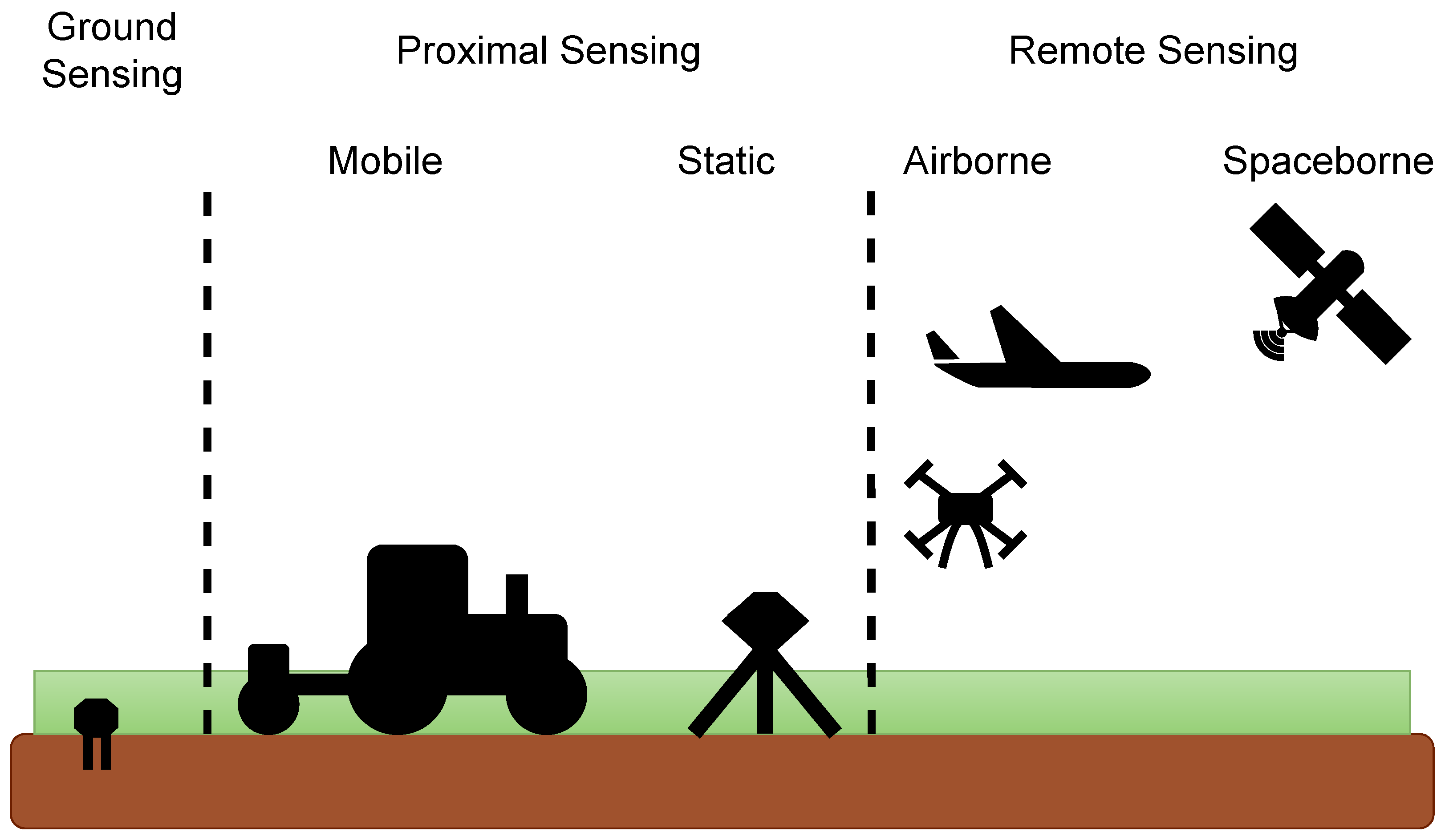
Non-invasive sensors are placed externally and without contact with the process to measure. They are called proximal sensors, where the instrument is placed within 2 m of the target, or remote sensors if the distance is greater [
10]. The main advantage against invasive techniques is the possibility of reading from different locations within a reasonable timeframe and naturally, not to touch nor affect the process. This ability to move the sensor allows overcoming the disadvantage of the invasive types with the small volume of the sample being measured.
Figure 1 shows the classification of Soil Moisture (SM) measurement methods. Non-invasive sensors are also easier to deploy and result in more stable results in harsh environments such as rocky or vertical soil, not depending on surface contacts.
Apart from RADAR, there are some other techniques for contactless measurement of the amount of moisture in the soil, each of which has its strengths and weaknesses.
Most non-invasive techniques to measure soil moisture imply using ElectroMagnetic (EM) radiation and measuring the soil’s reflected radiation. Common difficulties with non-invasive approaches include limited penetration depth (L-band microwave [
11]), difficulty in separating readings from different soil layers or depths (EMI, Cosmic Ray), soil moisture impacts the depth of the soil’s penetration (L-band microwave, EMI, Cosmic Ray, GPR), and the labor and effort required to perform such surveys (EMI and GPR) [
12].
1.1.1. Ground-Penetrating Radar
Ground-Penetrating Radar (GPR) is a non-invasive technique capable of mapping SM and is commonly used to detect buried objects (pipes, roots), voids, and cracks [
10].
GPR estimates the dielectric permittivity of the soil by transmitting electromagnetic waves and recording the travel time between a RADAR transmitter and receiver. The velocity of the EM wave in a specific medium is directly related to the dielectric permittivity, and therefore, one can estimate the SWC based on the electromagnetic waves’ travel time because of the large contrast between the dielectric permittivity of soil’s components: water, air and minerals [
13].
GPR devices can be operated on the soil surface or from off-ground (proximal) or airborne platforms (remote) [
14].
GPR can accurately measure soil moisture, reporting frequently a correlation above 0.93 with conventional soil sensors [
15,
16]. GPR is one of the few technologies that can map the SM variation in space [
12]. The term “map” relates to being feasible and practical to achieve a birds-eye 2D representation where each cell (in this case) has SM information. If a GPR-like system is used, each map cell will have a vector of soil moisture readings over depth. Some disadvantages are the time it takes to map the large areas and being prone to errors in saline soils [
9,
17].
1.1.2. Interferometric Reflectometry Systems
In general terms, Geographical Positioning System-Interferometric Reflectometry (GPS-IR) and Global Navigation Satellite System-Interferometric Reflectometry (GNSS-IR) use energy emitted elsewhere and capture the reflected signals from the ground, containing data about the surrounding environment [
18]. The SWC changes the reflected signal from altered soil’s permittivity and reflectivity [
19]. This way, the information about the soil moisture can be indirectly measured by analyzing the reflected signal [
18,
20].
Generically, GPS signals are situated in the so-called microwave part of the Radio Frequency (RF) spectrum [
11]. The particular frequency strongly influences the measurement depth of GPS-IR and GNSS-IR sensors; L-band microwaves reduce the penetration depth from 5 cm to a few millimeters (for high values of SWC) [
14,
21,
22]. The radius of the measuring area varies with the antenna height, achieving around 300 m, with the antenna at 20 m height [
21,
22].
The benefits of GPS-IR and GNSS-IR approaches in agriculture are the ability to use a commercial receiver with a modified antenna, the measurements range, and the high correlation with soil moisture sensors, with values above 0.90 [
23,
24]. Remote sensing GPR, such as GPS-IR and GNSS-IR, sensors have disadvantages such as the short depth measurements range, errors due to soil roughness, crop stubble, and vegetation biomass [
9,
19,
25].
1.1.3. ElectroMagnetic Induction
ElectroMagnetic Induction (EMI) devices were commonly used in agriculture to map significant soil variability or changes in soil type. EMI can also estimate soil salinity, texture, and clay content [
16,
26]. In any case, the demand for this technology is increasing in recent years due to interest in mapping SM in large areas [
12]. The increasing interest in this technology relates to the use of multifrequency and multi-coil EMI sensors and recent calibration algorithms [
26,
27,
28,
29].
EMI devices rely on the strong correlation between soil electrical conductivity and soil water content, unlike other approaches [
30]. These approaches apply an electric current to the soil using electromagnetic induction and then read the EM field that the ground generates [
14]. The amplitude and phase shift of the EM field created by the soil depends mainly on the moisture content and the concentration of ions in the soil. The space between the transmitter and the receiver coil and the distance to the ground also greatly influences the EM field created by the soil [
14].
EMI devices cannot directly measure SWC, and several soil parameters such as soil composition, temperature, salinity, and density influence the readings [
12]. Because electrical conductivity is correlated with several parameters, the relation between electrical conductivity and SWC is very complex and non-linear. Based on these points, solutions using only EMI in agriculture are not very likely to succeed [
12]. That is why many solutions tend to use EMI with GPR to measure soil moisture better [
30,
31].
1.2. Radio Detection AND Ranging (RADAR) Theory
Radio Detection And Ranging (RADAR) is a type of sensor that emits electromagnetic waves and then analyzes the reflected waves. Based on the type of signal the system emits, there are two categories: pulse RADAR and continuous wave RADAR [
32,
33].
1.2.1. Pulse RADAR
The pulse RADAR periodically emits short pulses of EM waves. The period between two consecutive pulses is related to the RADAR range. The period needs to be bigger than the time it takes for the waves to be emitted, reflected and received [
32,
33].
Ultra-WideBand (UWB) RADAR is a type of pulse RADAR that uses pulses of EME for a very brief period. To achieve that with good quality, expensive equipment is needed to send the pulses with high accuracy; high fidelity receiver electronics are also required to measure the reflection.
1.2.2. Continuous-Wave RADAR
Continuous-Wave (CW) RADAR is a type of RADAR where an EM wave with known frequency is emitted within a given medium (example: air) and reflected by any object (example: car). This method allows the removal of unrelated signals that, in turn, allows the reflected weak signals to be detected [
33,
34].
Without modulating the frequency, the sensor can not measure the distance of the objects due to the Doppler effect. Modulating the frequency allows having a better assessment of the object’s velocity and allows estimating the object’s position [
35].
Frequency-modulated continuous wave radar FMCW technology uses UWB RADARs’ components, i.e., the antennas, the voltage-controlled oscillators, and the low noise amplifiers, to make cost-effective RADARs with frequency bandwidths up to 4 GHz [
36].
1.3. Doppler Effect and Filter
When a fixed frequency wave hits a moving object, it will reflect the wave with a different frequency based on the relative velocity of the object to the wave’s transmitter. Suppose both object and RADAR have a velocity far inferior to the electromagnetic wave’s speed. In that case, the frequency’s shift is directly proportional to the relative velocity of the object relative to the emitter, and it is called the Doppler effect [
37].
PondView
The PondView diagram [
38] is a method to visualize and interpret GPR maps; this article will use this type of diagram for RADAR data. It allows the user to better identify buried objects and assess how deep the feature is.
PondView diagrams use thin horizontal slices taken from a map. They are usually only a few centimeters thick, containing the information of just one measurement from the GPR-like sensor. A thick slice is also possible by combining successive thin slices that can be vertically averaged or substituted by the vertical maximum.
PondView takes advantage of thick slices using the maximum method. It colorizes the thick slice with a two or three-color matrix based on the depth of each maximum. For the two-color pondView, the green is for shallower objects and blue is for deeper objects. The intensity of the color on each cell is based on the values of the measurements that need to be displayed; it is common that the actual data to be shown are based on differences to clarify the relevant data.
Summarizing, the PondView diagram deals with data that are 4D; that is, for each 2D cell (seen from above), the signal intensity over depth is at stake (a uni-dimensional vector of scalars). The shown color in each cell is related to the maximum difference of measurements just above and just below the depth at stake; saturated colors (far from black) relate to larger differences and, in turn, imply a medium change at that depth [
38].
2. Materials and Methods
This section characterizes the RADAR sensor for use in Soil Moisture measurement: the overall strategy of the experiments is to compare the RADAR readings in experiences with controlled soil moisture content. The controlled soil moisture content comes from contact sensors measurements and the experimental sequence itself.
2.1. Hardware Setup
The inexpensive FMCW RADAR used is a Texas Instruments AWR1843-BOOST [
39] RADAR. This board includes antennas and a serial connection to a device that will connect the data: in this research, a common low end PC. The AWR1843-BOOST is a FMCW RADAR with a frequency band of 77–81 GHz, three antennas, four receptors, and a range spatial resolution of 4 cm.
The RADAR is very versatile, allowing the configuration of several parameters such as the number of transmitters, receivers, and the field of view. The RADAR main characteristics are shown in
Table 1.
The used contact sensors are multiple DFRobot SEN0193 sensors [
40] and a AM2302 [
41] temperature–humidity sensor. The SEN0193 is a gravity analog capacitive soil moisture sensor that reads the moisture by capacitive sensing. We chose this well-known, widely used sensor [
42,
43,
44] because capacitive sensors are immune to effects such as soil’s evapotranspiration [
45], and this one has acceptable accuracy, with a correlation coefficient (R
2) minimum of 0.91 [
43]. The measurements from the SEN0193 were collected using an Arduino Uno and sent to a computer.
2.2. Data Representation and Analysis
The Spearman coefficient was used to analyze the correlation between the measurements from the capacitive soil moisture sensors and data from the RADAR sensor. This method evaluates the monotonic relationship between two series. A monotonic relationship is a relationship that does one of the following:
When one series increases, the other increases as well;
When one series increases, the other decreases.
Since the ground-truth signal is far from having a linear correlation with the SWC [
42], the non-parametric Spearman coefficient is well suited because the rates of increasing/decreasing of the series do not need to be constant. In contrast, in a linear relationship, the rate of increase/decrease is constant.
Since the signals from the RADAR and from the control signal (SEN0193 sensor) can be out of sync, a Cross-Correlation Function (CCF) allows to better assess the correlation between the two sensors, taking into consideration potential delays [
46]. The delays are most likely related to water spread time in the soil. This CCF measures the similarity between possibily related signals that might include an unknown delay. This way, the same correlation algorithm gives the highest value of correlation as well as it allows to estimate the delay that maximizes the correlation [
46].
2.3. Preparation of Experiences—Soil Tests And Sensing
Four experiments were carried out to ascertain the performance and quality of the RADAR sensor. Different types of containers were used according to the measurements made with the sensors. Each reading from the RADAR is an average of three consecutive measurements.
2.3.1. Experiment 1—One-Layer Soil
Experiment one was performed in a clay vase measuring 23 cm diameter and 21 cm height. One soil moisture sensor was inserted at 2 cm depth, and a temperature–humidity sensor was placed above the experiment. The soil is composed of just one layer of 18 cm thickness, and it represents fertile agricultural soil (rich nutrients and organic matter) without fertilizers.
We intended to test a correlation between the RADAR’s signal and the soil water content derived from the capacitive soil moisture sensor. The RADAR was positioned at 9 cm from the soil. We used a sample period of 30 s for the soil moisture sensor one minute for the RADAR.
2.3.2. Experiments 2—Three-Layer Soil
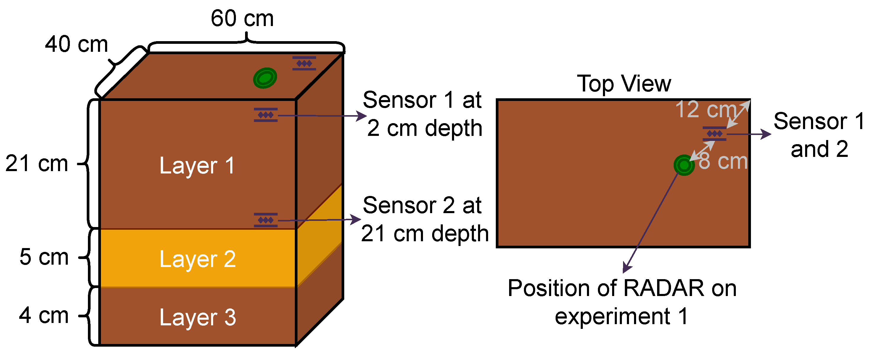
Experiment two was conducted in a plastic container measuring approximately 40 × 60 × 35 cm3. This experiment aims to assess if the size or type of the container influences the readings and if the RADAR can measure the soil moisture at a deeper level.
The soil is composed of three layers. The first layer (the top) is 21 cm high, with the same soil composition as the previous experiment. The second layer is 5 cm in height with fewer nutrients, a higher concentration of sand, and a much higher apparent or bulk density. The third layer (bottom) is 4 cm high and is equal to the first layer. The position of the sensors is shown in
Figure 2. The ground-truth sensor is 2.3 × 9.8 cm
2 in size, which makes it small compared to the volume of soil in the experiment. Thus, it is assumed that its presence is negligible in terms of general SWC; experiments demonstrate that the sensor is outside of the cone of RADAR detection.
Two soil moisture sensors were inserted at different depths for experiments one and two, one at 2 cm and the other at 21 cm underground, as shown in
Figure 2. The RADAR was 9 cm away from the soil. We used a sample period of 100 s for the soil moisture sensor and five minutes for the RADAR during 36 h in the same position. This way, there are two intermediate readings from the control signal between two sequential readings from the RADAR.
2.3.3. Experiment 3—Oven-Dried Soil with One Layer
Experiment three was in a plastic container measuring 15 cm diameter, 25 cm height and the top was sealed. The container had the RADAR and the temperature–humidity sensor inside. One soil moisture sensor was inserted at 2 cm depth. The objective of this experiment is to assess in what interval of SWC the RADAR has the best performance.
The soil is composed of just one layer 13 cm high and with the composition of experiment 1 (fertile soil taken from the same bag from a well-known commercial brand). The soil was dried in an oven with a temperature between 105 and 110 ºC to get practically 0% SWC.
As mentioned earlier, the air’s moisture inside the covered container is measured by a specific sensor. The container is always fully sealed (no air nor moisture exchange), and all the sensors are inside the enclosed volume. The periodic addition of water is made with a syringe that crosses the top seal made of plastic wrap. In addition, the tiny hole is sealed to prevent any exchange to the interior.
2.3.4. Experiment 4—Three-Layer Soil Mapping
The fourth experiment is the collection of the readings in a squared grid with 4 ± 0.1 cm of pace. For that, a CNC-like manipulator was used. This manipulator was based on a commercial product called AxiDraw [
47], and its design can be found in Thingiverse [
48].
Each reading from the RADAR is an average of three consecutive measurements at 16 cm of distance from the soil and with constant room temperature. The manipulator takes less than half a second to move between positions.
Table 2 summarizes the main characteristics of each experiment.
3. Results and Discussion
We conducted four experiments to analyze the useability of the RADAR as a method to assess SWC. We evaluated the RADAR’s signal versus the ground-truth value in a small container, experiment 1, and in a big container, experiment 2. Then, we decided to assess the conditions where the RADAR had the best outcomes, resulting in experience 3. We tried to map the SWC in the big container to finalize it, as shown in experience 4.
3.1. First Experiment
In the first experiment, we intended to test a correlation between the RADAR’s signal and the soil water content derived from the capacitive soil moisture sensor. To achieve the goals of this experiment, we recorded the data from the sensors for more than an hour, without changing the soil and the sensor’s conditions, to acquire the values for the soil’s state. After that, we added to the soil 300 mL of water directly below the RADAR.
We arranged the readings to make a graphic of the RADAR’s signal, soil humidity sensor signal, temperature, and humidity of the air by the time to see the evolution of the RADAR’s signal over time and compare it to the rest of the data.
Figure 3 presents the results from two runs of this experiment.
Both derived soil moisture sensing techniques strongly respond to the water-added event, showing sharp readings fall. The sensors’ signal reached a minimum, which was followed by a consistent signal increase in a short period, likely related to water drainage. After this period, the soil moisture sensors behave differently. While the RADAR sensor shows a time profile toward signal stability or even descent, the capacitive sensor, in both experiments, shows a clear tendency toward a signal increase. In this period, the temporal pattern of the RADAR sensor signal is similar to the humidity sensor signal and quite different from the capacitive sensor time profile. After adding water, the temperature and soil moisture show a distinct evolution in both experiments. In one of the situations, the temperature has a tendency to rise and the humidity has a tendency to decrease. Whilst in another experiment, these variables show a contrary trend after adding water. Soil moisture sensor capacitance-based seems to be affected by the soil temperature, as reported previously by Oates et al. [
13].
The calculated Spearman’s correlation between the signals of both sensors yields 0.78. Meanwhile, the cross-correlation function (CCF) between the signals of both sensors yields 0.94 with a 5 min delay.
3.2. Second Experiment
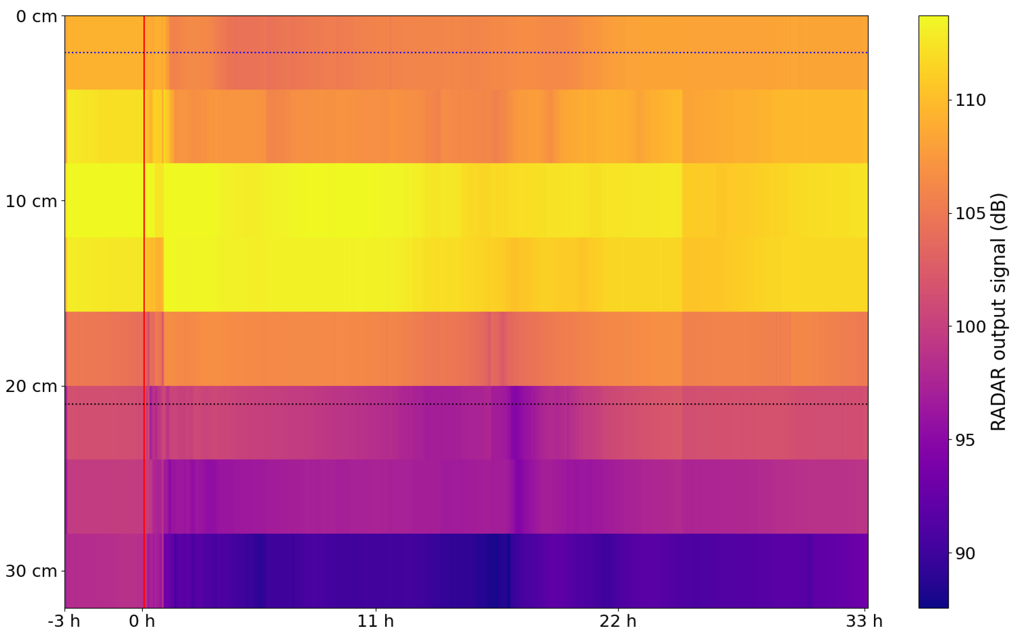
The main objective of this experiment is to analyze if the RADAR could be used for soil moisture monitoring.
To achieve the goals of this experiment, we recorded the data from the sensors for three and a half hours, without changing the soil and the sensor’s conditions, to acquire the values for dry soil. After that, we added to the soil 500 mL of water, directly below the RADAR, without saturating the soil.
We mapped the measurements from the RADAR into colors based on the signal’s intensity. Then, we arranged the readings to make a graphic of depth by the time to see the evolution of the RADAR’s signal over time.
Figure 4 presents the results from this experiment.
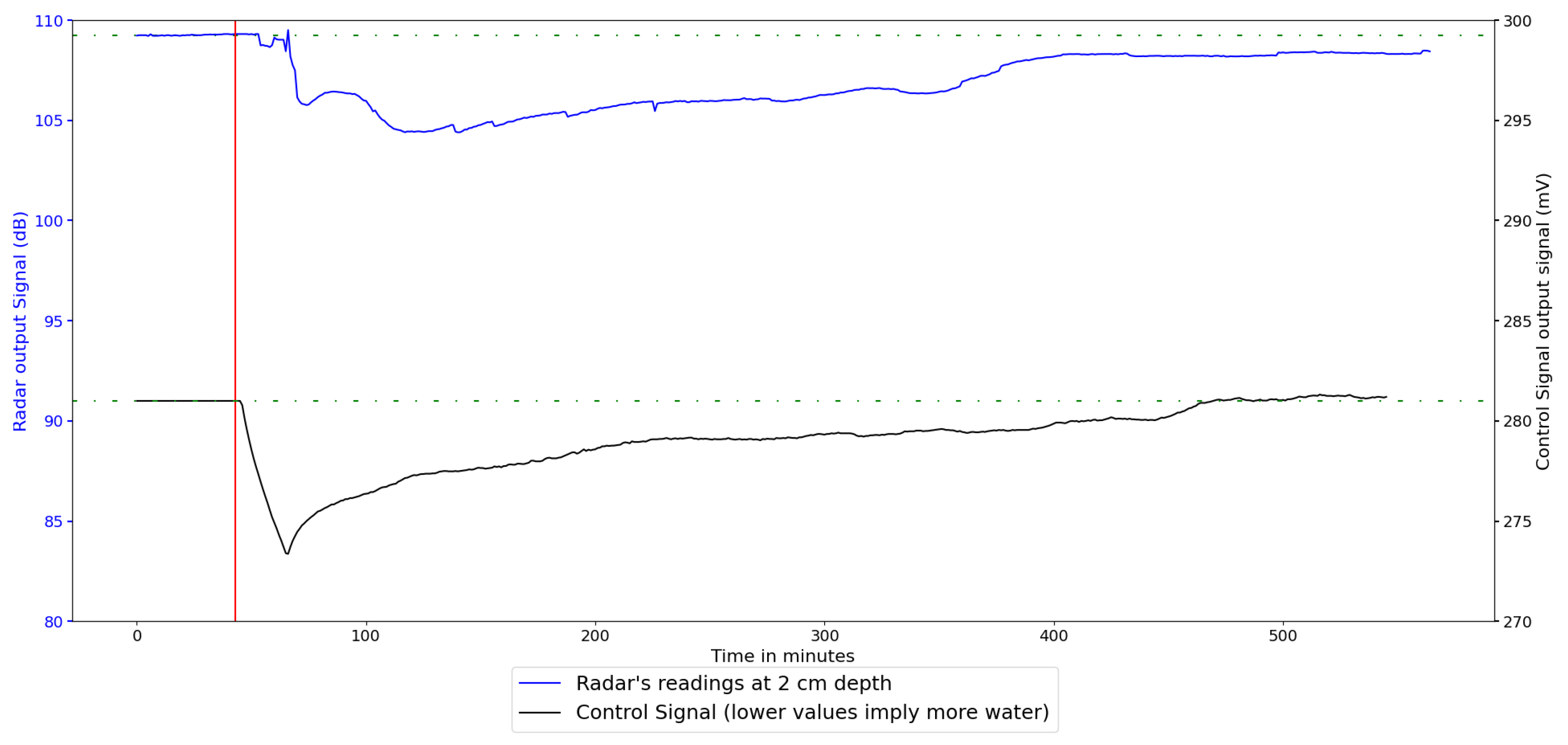
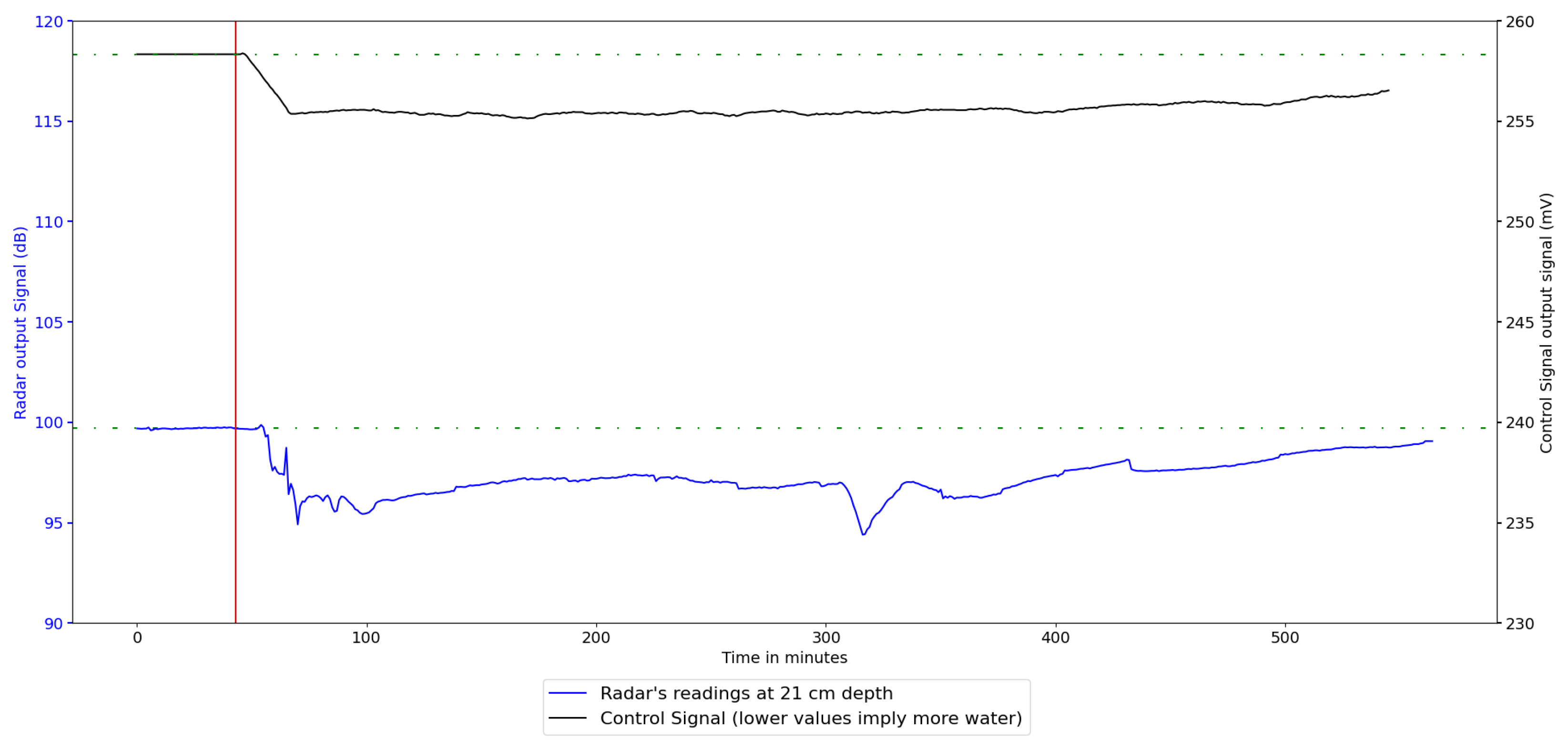
To compare the soil moisture sensor’s and the RADAR’s readings, we extracted the values from the RADAR at the same depth as the other sensors, producing
Figure 5 and
Figure 6. These figures show that the more water the soil has, the lower the RADAR’s signal intensity. This relation is due to the water having a much bigger dielectric constant than the soil.
We calculated Spearman’s correlation between the signals of both sensors, giving 0.75 and 0.64 at a depth of 2 cm and 21 cm, correspondingly. Near the surface, the correlation is lower due to the water, making the soil and the sediments more compact, even after it dries, increasing both RADAR readings. This can be seen in
Figure 6, where the soil moisture sensor near-surface ends with a higher value than moments before adding water.
We also calculated the cross-correlation function (CCF) between the signals of both sensors. At a depth of 2 cm, the maximum value of correlation was 0.73 with a delay of 21 min and at depth of 21 cm, the maximum value of correlation was 0.82 without any delay.
The RADAR sensor could not detect the three different sediment layers used in our experiments. Nevertheless, the effect on water absorption and evaporation is relevant. The layers have different compositions, densities, and water absorption capabilities. That discontinuity in soil characteristics is likely to create additional small water pockets between soil layers when water is added. Small condensation zones between soil layers appear when the water evaporates. These phenomena are the most likely explanation why the RADAR’s readings at 21 cm depth show some peaks and valleys throughout the experiment 2. The soil moisture sensor does not show this change because the capacitive sensing principle makes them not sensitive to condensation.
3.3. Third Experiment
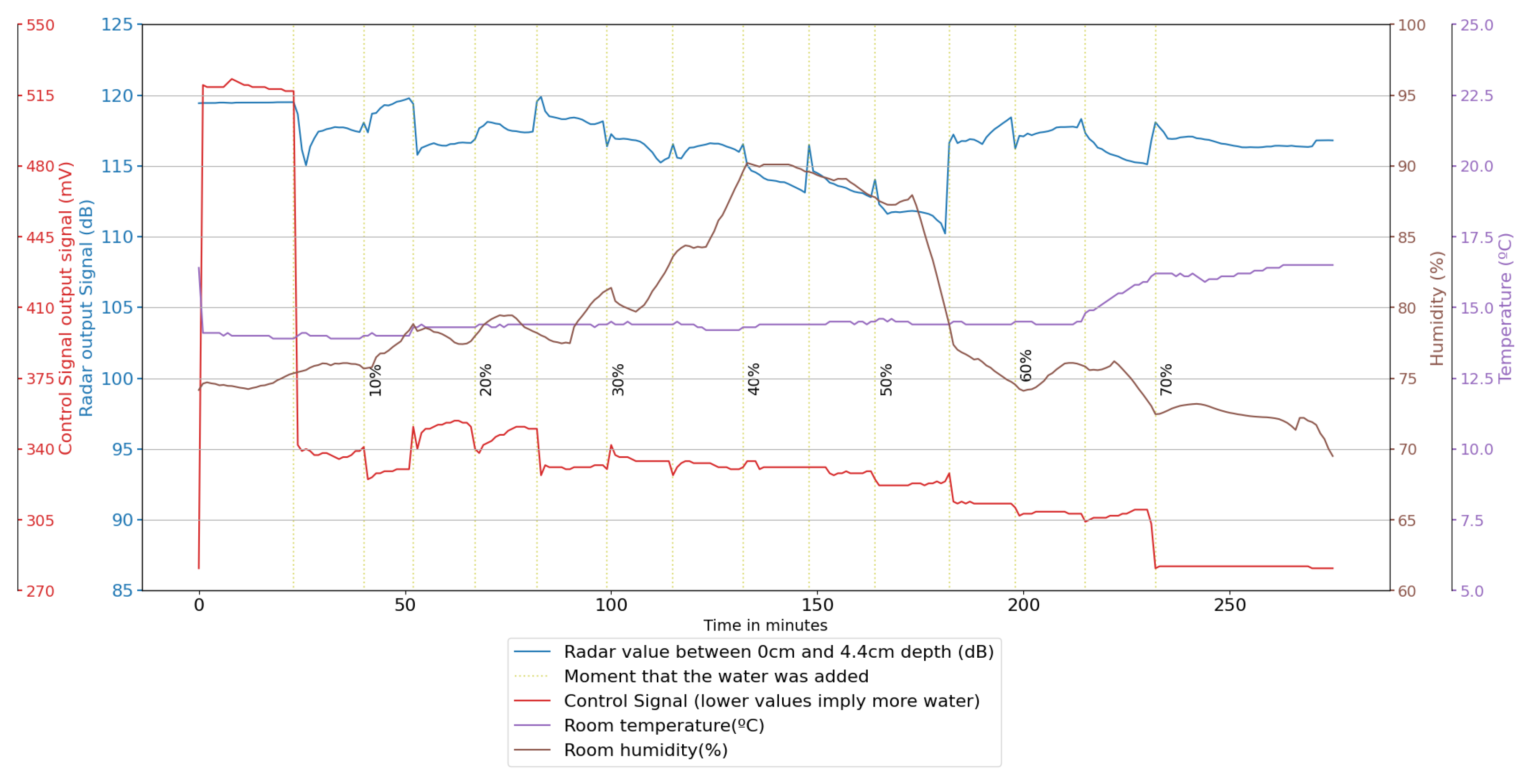
To assess the conditions that gave the best results, we recorded the data from the sensors sealed inside the plastic container for half an hour, without changing the soil and the sensor’s conditions, to acquire the values for dry soil. This record was shorter than in the other experiments because we know the previous state of the soil. After the waiting period, we added 5% water in mass to the soil four times per hour, directly below the RADAR.
We arranged the readings to make a graphic of the RADAR’s signal, control signal, temperature, and humidity of the air by the time to see the evolution of the RADAR’s signal over time and compare it to the rest of the data.
Figure 7 presents two results from this experiment.
Figure 7 shows that the effect of SWC in the RADAR’s readings is not constant. When the SWC is high enough, the RADAR’s signal, instead of decreasing, increases with SWC. With elevated SWC, the soil gets to the point that it cannot absorb water anymore, making the water reflect the RADAR’s signal.
3.4. Fourth Experiment
The fourth experiment intends further to test the correlation between the RADAR’s signal and the SWC in an experiment that maps the soil that would be viewed in bird’s eye view as 2D. For visualization, the pondView strategy is used.
We recorded the data from the RADAR with a top view horizontal square grid of 4 cm spacing before adding 1 L of water to the soil and one hour after it. This way, we have a map with the dry soil and another for the wet soil.
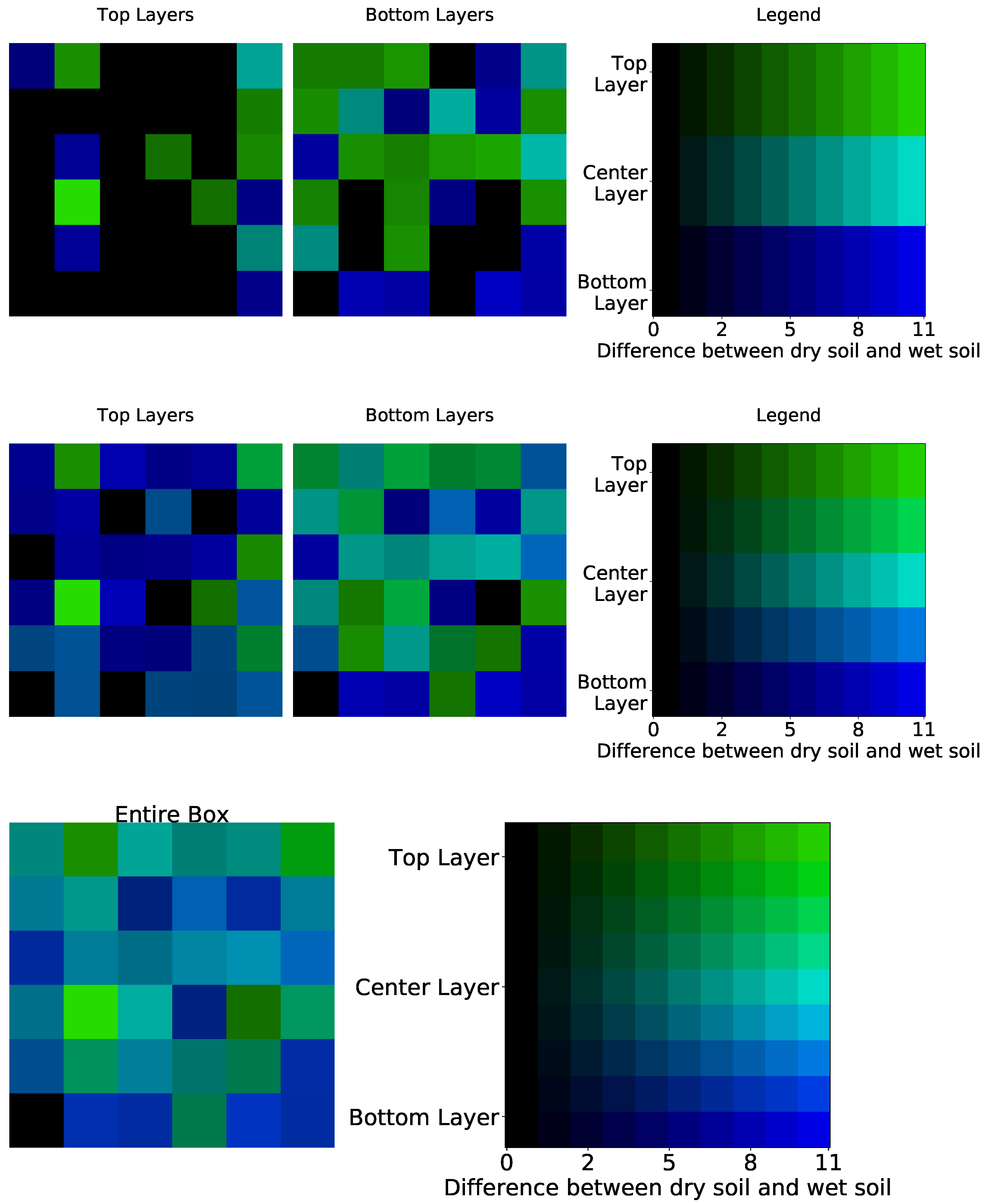
We created three pondViews based on the RADAR’s readings. One pondView shows the difference between dry and wet soil near the surface, and the other shows the same difference but deeper.
Figure 8 shows the three pondView diagrams, showing different numbers of layers.
Because the presence of water in the soil lowers the intensity of the signal read by the RADAR, it is only interesting to analyze the positive values of the difference between dry and wet soil.
Figure 8 shows several pondViews with different parameters. In the near-surface pondViews, we can see that the most significant difference is between 12 and 20 cm deep because the pondView with just three layers shows not so many changes and the pondView with five layers is predominantly blue. The reason is that since we add water to the ground, gravity tends to push the water into lower levels. In the deeper pondView, we can see that the significant differences are around 24 cm depth due to two factors. The three-layer pondView has a lot of greens (24 cm depth layer’s color). The five-layer pondView has a significant concentration of cyan (24 cm depth layer’s color) and light green and light blue. Analyzing the entire box pondView, we can see that it is predominantly light blues (24 and 28 cm depth layer’s colors), corroborating what was previously said in the experience before and what the other pondViews indicate.
4. Conclusions and Future Work
The results of this research show that the inexpensive automotive FMCW RADAR (AWR1843-BOOST) is a cost-effective alternative for GPR to assess near-surface water content in the soil (under certain constraints). Such results show that the tested sensor (and its cost-effective working principle) are able to determine soil water content (within certain limitations) in a non-intrusive, proximal sensing manner. “Direct” readings are usable for Soil Moisture below 15%. This limitation is severe, but nonetheless, the sensor is very useful for agricultural purposes, for instance to control precision irrigation schedules, leading to cost-efficient management of scarce water resources. Once perfected, this on-the-go sensor will be highly suitable for mapping crop water management in line with precision agriculture. As with many other sensors, it must be recognized that specific readings are likely to be dependent on the soil properties, but simple calibration procedures will avoid that shortcoming.
These results were obtained without the real-time data capture adapter DCA1000EVM of the AWR1843-BOOST. The use of this adapter is likely to improve results (at the cost of slightly more expensive hardware), and this can be done in the future, when the device become available. In addition, additional experiments are needed to ascertain the real precision of the measurements with different soils at higher depths and over increasing depths.
Non-intrusive SWC assessment is especially interesting in applications such as SWC mapping (where the sensor is transported by any kind of mobile device) or in situations where implementing intrusive sensors is not possible, such as rocky soil or vertical surfaces. The use of non-intrusive sensors in mobile machines or robots is likely to enable the acquisition of ground observations to investigate soil moisture–climate interactions.
Author Contributions
Conceptualization, R.M.C., A.S. and F.S.; Data curation, M.C.; Formal analysis, R.M.C. and M.C.; Funding acquisition, A.S. and F.S.; Investigation, R.M.C.; Methodology, R.M.C. and M.C.; Project administration, A.S., F.S. and M.C.; Software, R.M.C.; Supervision, A.S., F.S. and M.C.; Validation, A.S., F.S. and M.C.; Writing—original draft, R.M.C. and A.S.; Writing—review & editing, R.M.C., A.S., F.S. and M.C. All authors have read and agreed to the published version of the manuscript.
Funding
This work is financed by the ERDF—European Regional Development Fund, through the Operational Programme for Competitiveness and Internationalisation—COMPETE 2020 Programme under the Portugal 2020 Partnership Agreement within project Replant, with reference POCI-01-0247-FEDER-046081.
Institutional Review Board Statement
Not applicable.
Informed Consent Statement
Not applicable.
Data Availability Statement
Conflicts of Interest
The authors declare no conflict of interest.
Abbreviations
The following abbreviations are used in this manuscript:
| USGS | United States Geological Survey |
| WUE | Water Use Efficiency |
| SWC | Surface Water Content |
| RADAR | Radio Detecting And Ranging |
| EME | Eletromagnetic Energy |
| FMCW | Frequency Modulated Continuous Wave |
| SM | Soil Moisture |
| EM | Electromagnetic |
| EMI | Eletromagnetic Induction |
| GPS-IR | Geographical Positioning System Interferometric Reflectometry |
| GNSS-IR | Global Navigation Satellite System Interferometric Reflectometry |
| RF | Radio Frequency |
| UWB | Ultra-Wideband |
| PC | Personal Computer |
| CNC | Computerized Numerical Control |
References
- Sheffield, J.; Wood, E.F. Global Trends and Variability in Soil Moisture and Drought Characteristics, 1950–2000, from Observation-Driven Simulations of the Terrestrial Hydrologic Cycle. J. Clim. 2008, 21, 432–458. [Google Scholar] [CrossRef] [Green Version]
- Samaniego, L.; Thober, S.; Kumar, R.; Wanders, N.; Rakovec, O.; Pan, M.; Zink, M.; Sheffield, J.; Wood, E.F.; Marx, A. Anthropogenic warming exacerbates European soil moisture droughts. Nat. Clim. Chang. 2018, 8, 421–426. [Google Scholar] [CrossRef]
- Seneviratne, S.I.; Corti, T.; Davin, E.L.; Hirschi, M.; Jaeger, E.B.; Lehner, I.; Orlowsky, B.; Teuling, A.J. Investigating soil moisture–climate interactions in a changing climate: A review. Earth-Sci. Rev. 2010, 99, 125–161. [Google Scholar] [CrossRef]
- Dirmeyer, P.A. The terrestrial segment of soil moisture–climate coupling. Geophys. Res. Lett. 2011, 38. [Google Scholar] [CrossRef]
- Oki, T.; Kanae, S. Global Hydrological Cycles and World Water Resources. Science 2006, 313, 1068–1072. [Google Scholar] [CrossRef] [Green Version]
- Li, S.; Pezeshki, S.; Goodwin, S. Effects of soil moisture regimes on photosynthesis and growth in cattail (Typha latifolia). Acta Oecol. 2004, 25, 17–22. [Google Scholar] [CrossRef]
- Srivastava, P.K. Satellite Soil Moisture: Review of Theory and Applications in Water Resources. Water Resour. Manag. 2017, 31, 3161–3176. [Google Scholar] [CrossRef]
- De Mahieu, A.; Ponette, Q.; Mounir, F.; Lambot, S. Using GPR to analyze regeneration success of cork oaks in the Maâmora forest (Morocco). NDT E Int. 2020, 115, 102297. [Google Scholar] [CrossRef]
- Klotzsche, A.; Jonard, F.; Looms, M.; Van Der Kruk, J.; Huisman, J. Measuring Soil Water Content with Ground Penetrating Radar: A Decade of Progress. Vadose Zone J. 2018, 17, 180052. [Google Scholar] [CrossRef] [Green Version]
- Viscarra Rossel, R.; Mcbratney, A.; Minasny, B. Proximal Soil Sensing; Sringer: Berlin/Heidelberg, Germany, 2010. [Google Scholar] [CrossRef]
- ESA—Satellite Frequency Bands. Available online: https://www.esa.int/Applications/Telecommunications_Integrated_Applications/Satellite_frequency_bands (accessed on 12 December 2021).
- Hardie, M. Review of Novel and Emerging Proximal Soil Moisture Sensors for Use in Agriculture. Sensors 2020, 20, 6934. [Google Scholar] [CrossRef]
- Oates, M.; Ramadan, K.; Molina-Martínez, J.; Ruiz-Canales, A. Automatic fault detection in a low cost frequency domain (capacitance based) soil moisture sensor. Agric. Water Manag. 2017, 183, 41–48. [Google Scholar] [CrossRef]
- Babaeian, E.; Sadeghi, M.; Jones, S.B.; Montzka, C.; Vereecken, H.; Tuller, M. Ground, Proximal, and Satellite Remote Sensing of Soil Moisture. Rev. Geophys. 2019, 57, 530–616. [Google Scholar] [CrossRef] [Green Version]
- Liu, X.; Cui, X.; Guo, L.; Chen, J.; Li, W.; Yang, D.; Cao, X.; Chen, X.; Liu, Q.; Lin, H. Non-invasive estimation of root zone soil moisture from coarse root reflections in ground-penetrating radar images. Plant Soil 2019, 436, 623–639. [Google Scholar] [CrossRef]
- Toy, C.W.; Steelman, C.M.; Endres, A.L. Comparing electromagnetic induction and ground penetrating radar techniques for estimating soil moisture content. In Proceedings of the XIII Internarional Conference on Ground Penetrating Radar, Lecce, Italy, 21–25 June 2010. [Google Scholar] [CrossRef]
- Susha Lekshmi, S.U.; Singh, D.; Baghini, M.S. A critical review of soil moisture measurement. Measurement 2014, 54, 92–105. [Google Scholar] [CrossRef]
- Chang, X.; Jin, T.; Yu, K.; Li, Y.; Li, J.; Zhang, Q. Soil Moisture Estimation by GNSS Multipath Signal. Remote Sens. 2019, 11, 2559. [Google Scholar] [CrossRef] [Green Version]
- Zhang, L.; Lu, T.; Yu, P.; Zhang, C. Parameter Measurement of Soil Moisture based on GNSS-R Signals. In Proceedings of the 2019 IEEE International Conference on Artificial Intelligence and Computer Applications (ICAICA), Dalian, China, 29–31 March 2019. [Google Scholar] [CrossRef]
- Larson, K.M.; Small, E.E.; Gutmann, E.D.; Bilich, A.L.; Braun, J.J.; Zavorotny, V.U. Use of GPS receivers as a soil moisture network for water cycle studies. Geophys. Res. Lett. 2008, 35. [Google Scholar] [CrossRef] [Green Version]
- Bogena, H.R.; Huisman, J.A.; Güntner, A.; Hübner, C.; Kusche, J.; Jonard, F.; Vey, S.; Vereecken, H. Emerging methods for noninvasive sensing of soil moisture dynamics from field to catchment scale: A review. WIREs Water 2015, 2, 635–647. [Google Scholar] [CrossRef] [Green Version]
- Larson, K.M.; Braun, J.J.; Small, E.E.; Zavorotny, V.U.; Gutmann, E.D.; Bilich, A.L. GPS Multipath and Its Relation to Near-Surface Soil Moisture Content. IEEE J. Sel. Top. Appl. Earth Obs. Remote Sens. 2010, 3, 91–99. [Google Scholar] [CrossRef]
- Koch, F.; Schlenz, F.; Prasch, M.; Appel, F.; Ruf, T.; Mauser, W. Soil Moisture Retrieval Based on GPS Signal Strength Attenuation. Water 2016, 8, 276. [Google Scholar] [CrossRef]
- Han, M.; Zhu, Y.; Yang, D.; Hong, X.; Song, S. A Semi-Empirical SNR Model for Soil Moisture Retrieval Using GNSS SNR Data. Remote Sens. 2018, 10, 280. [Google Scholar] [CrossRef] [Green Version]
- Zhang, S.; Calvet, J.C.; Darrozes, J.; Roussel, N.; Frappart, F.; Bouhours, G. Deriving surface soil moisture from reflected GNSS signal observations from a grassland site in southwestern France. Hydrol. Earth Syst. Sci. 2018, 22, 1931–1946. [Google Scholar] [CrossRef] [Green Version]
- Badewa, E.; Unc, A.; Cheema, M.; Kavanagh, V.; Galagedara, L. Soil Moisture Mapping Using Multi-Frequency and Multi-Coil Electromagnetic Induction Sensors on Managed Podzols. Agronomy 2018, 8, 224. [Google Scholar] [CrossRef] [Green Version]
- Shanahan, P.W.; Binley, A.; Whalley, W.R.; Watts, C.W. The Use of Electromagnetic Induction to Monitor Changes in Soil Moisture Profiles beneath Different Wheat Genotypes. Soil Sci. Soc. Am. J. 2015, 79, 459–466. [Google Scholar] [CrossRef] [Green Version]
- Lu, C.; Zhou, Z.; Zhu, Q.; Lai, X.; Liao, K. Using residual analysis in electromagnetic induction data interpretation to improve the prediction of soil properties. CATENA 2017, 149, 176–184. [Google Scholar] [CrossRef]
- Wang, H.; Wellmann, F.; Zhang, T.; Schaaf, A.; Kanig, R.M.; Verweij, E.; Hebel, C.; Kruk, J. Pattern Extraction of Topsoil and Subsoil Heterogeneity and Soil-Crop Interaction Using Unsupervised Bayesian Machine Learning: An Application to Satellite-Derived NDVI Time Series and Electromagnetic Induction Measurements. J. Geophys. Res. Biogeosci. 2019, 124, 1524–1544. [Google Scholar] [CrossRef]
- Moghadas, D.; André, F.; Slob, E.C.; Vereecken, H.; Lambot, S. Joint full-waveform analysis of off-ground zero-offset ground penetrating radar and electromagnetic induction synthetic data for estimating soil electrical properties. Geophys. J. Int. 2010, 182, 1267–1278. [Google Scholar] [CrossRef] [Green Version]
- André, F.; Van Leeuwen, C.; Saussez, S.; Van Durmen, R.; Bogaert, P.; Moghadas, D.; De Rességuier, L.; Delvaux, B.; Vereecken, H.; Lambot, S. High-resolution imaging of a vineyard in south of France using ground-penetrating radar, electromagnetic induction and electrical resistivity tomography. J. Appl. Geophys. 2012, 78, 113–122. [Google Scholar] [CrossRef]
- Radar Systems Tutorial. Available online: https://www.tutorialspoint.com/radar_systems/index.htm (accessed on 28 April 2022).
- Wolff, C. Doppler Filter. Available online: https://www.radartutorial.eu/11.coherent/Doppler-Filter.en.html (accessed on 12 December 2021).
- Khan, R.; Power, D. Aircraft detection and tracking with high frequency radar. In Proceedings of the International Radar Conference, Alexandria, VA, USA, 8–11 May 1995; pp. 44–48. [Google Scholar] [CrossRef]
- Cook, C.E.; Bernfeld, M. Radar Signals: An Introduction to Theory and Application; Artech House: Boston, MA, USA, 1993. [Google Scholar]
- Maaref, N.; Millot, P.; Pichot, C.; Picon, O. Ultra-wideband Frequency Modulated Continuous Wave synthetic aperture radar for Through-The-Wall localization. In Proceedings of the 2009 European Radar Conference (EuRAD), Rome, Italy, 30 September–2 October 2009; pp. 609–612. [Google Scholar]
- McGregor, J.D.; Silva, R.S.; Almeida, E.S. Architectures of Transportation Cyber-Physical Systems; Elsevier: Amsterdam, The Netherlands, 2018; Chapter 2; pp. 21–49. [Google Scholar] [CrossRef]
- Grasmueck, M.; Viggiano, D. PondView: Intuitive and Efficient Visualization of 3D GPR Data. In Proceedings of the 17th International Conference on Ground Penetrating Radar (GPR), Rapperswil, Switzerland, 18–21 June 2018. [Google Scholar] [CrossRef]
- IWR1843BOOST Evaluation Board|TI.com. Available online: https://www.ti.com/tool/IWR1843BOOST (accessed on 12 December 2021).
- Capacitive Soil Moisture Sensor SKU SEN0193 DFRobot. Available online: https://wiki.dfrobot.com/Capacitive_Soil_Moisture_Sensor_SKU_SEN0193 (accessed on 12 December 2021).
- Adafruit. AM2302 (Wired DHT22) Temperature-Humidity Sensor. Available online: https://www.adafruit.com/product/393 (accessed on 12 December 2021).
- Nagahage, E.A.A.D.; Nagahage, I.S.P.; Fujino, T. Calibration and Validation of a Low-Cost Capacitive Moisture Sensor to Integrate the Automated Soil Moisture Monitoring System. Agriculture 2019, 9, 141. [Google Scholar] [CrossRef] [Green Version]
- Radi; Murtiningrum; Ngadisih; Muzdrikah, F.S.; Nuha, M.S.; Rizqi, F.A. Calibration of Capacitive Soil Moisture Sensor (SKU:SEN0193). In Proceedings of the 4th International Conference on Science and Technology (ICST), Yogyakarta, Indonesia, 7–8 August 2018; pp. 1–6. [Google Scholar] [CrossRef]
- Sofwan, A.; Sumardi, S.; Ahmada, A.I.; Ibrahim, I.; Budiraharjo, K.; Karno, K. Smart Greetthings: Smart Greenhouse Based on Internet of Things for Environmental Engineering. In Proceedings of the International Conference on Smart Technology and Applications (ICoSTA), Surabaya, Indonesia, 20 February 2020; pp. 1–5. [Google Scholar] [CrossRef]
- Li, M. Humidity Sensors—Resistive or Capacitive? Available online: https://www.zhinst.com/europe/en/blogs/humidity-sensors-resistive-or-capacitive-mfia-can-tell-answer (accessed on 12 December 2021).
- Hayes, A. Cross-Correlation. Available online: https://www.investopedia.com/terms/c/crosscorrelation.asp (accessed on 29 April 2021).
- AxiDraw Writing and Drawing Machines. Available online: https://www.axidraw.com/ (accessed on 12 December 2021).
- Drawing Robot—Arduino Uno + CNC Shield + GRBL by henryarnold—Thingiverse. Available online: https://www.thingiverse.com/thing:2349232 (accessed on 12 December 2021).
| Publisher’s Note: MDPI stays neutral with regard to jurisdictional claims in published maps and institutional affiliations. |
© 2022 by the authors. Licensee MDPI, Basel, Switzerland. This article is an open access article distributed under the terms and conditions of the Creative Commons Attribution (CC BY) license (https://creativecommons.org/licenses/by/4.0/).


