Ensemble-Learning-Based Prediction of Steel Bridge Deck Defect Condition

Abstract

This study developed an ensemble-learning-based bridge deck defect condition prediction model to help bridge managers make more rational and informed steel bridge deck maintenance decisions. Using the latest data from the NBI database for 2021, this study first used ADASYN to solve imbalance problems in the data, then built six ensemble learning models (RandomForest, ExtraTree, AdaBoost, GBDT, XGBoost, and LightGBM) and used a grid search method to determine the hyperparameters of the models. The optimal model was finally analyzed using the interpretable machine learning framework, SHAP. The results show that the optimal model is XGBoost, with an accuracy of 0.9495, an AUC of 0.9026, and an F1-Score of 0.9740. The most important factor affecting the condition of steel bridge deck defects is the condition of the bridge’s superstructure. In contrast, the condition of the bridge substructure and the year of bridge construction are relatively minor factors.

1. Introduction

With the advantages of a large span, a short construction period, and easy transportation, steel bridges have been widely used in bridge engineering. Among the various components of steel bridges, bridge decks are more prone to defects than other components during service because they are directly subjected to traffic loads [1]. Under the influence of various factors such as vehicle load and climatic environment, steel bridge decks will experience different degrees of defects. Cracking, rutting, and other types of fatigue damage, such as fatigue cracks, are the most typical steel bridge deck defects [2,3]. If fatigue cracks are not treated in time, they will lead to water and other chemical reagents and steel bridge panel contact [4]. The steel bridge panel will produce corrosion phenomena, thus affecting the performance of the bridge deck. Severe cracking will also increase the roughness of the bridge deck, affecting driving comfort and safety [5]. Compared with the rapid progress in construction in China, the management and maintenance technology for such projects are relatively underdeveloped. After defects appear on the bridge deck, domestic bridge management is prone to incorrectly predicting the condition of defects and the future development trends, making it difficult to carry out effective maintenance measures. Therefore, it is essential to carry out research related to identifying defects in steel bridge decks. In recent years, large-span steel bridges have been widely used in China, but the proportion of the overall number of bridges is still small, and most of them are in the early stages of service. Usually, large amounts of data are needed to analyze the defective condition of in-service steel bridge decks. It is difficult to collect data related to steel bridge decks in China. The United States has more developed transportation infrastructure. National Bridge Information Base (NBI) data show that the number of steel bridges in the United States will account for more than 30% of the bridges in the country by 2021 [6]. The NBI is a database compiled by the Federal Highway Administration that contains data related to the structure type, material type, and condition rating of bridges in each state of the United States [7]. All of the data are recorded in a uniform standard. Therefore, using the NBI database can provide good data support for predicting and analyzing steel bridge deck defect conditions. Developing a data-driven prediction model can help Chinese bridge managers make better deck maintenance decisions.

To build a bridge deck defect condition prediction model, it is necessary to establish the interrelationships between deck conditions and various parameters (such as superstructure condition, substructure condition, average daily traffic, structure length, bridge roadway width, and bridge age) of the bridge, but there are significant challenges to making such a model due to the highly nonlinear relationship between the parameters [8,9,10]. However, with the rapid development of artificial intelligence in the last decade, many researchers have started to use machine learning models to solve related problems in the field of civil engineering [11]. Regarding the issue of bridge deck condition prediction, Ghonima et al. used stochastic parametric binary logistic regression to predict the effects of environmental and structural parameters on the bridge deck condition [12]. They showed that the developed stochastic parametric model outperformed the traditional binary logistic model. Lavrenz et al. used the multivariate three-stage least squares model to predict the condition of the bridge deck, superstructure, and substructure conditions [13]. They compared it with the ordinary least squares model, and the results showed that the multivariate three-stage least squares model had higher accuracy. Ranjith et al. used a stochastic Markov chain model to predict the condition of wooden bridges [14]. The results showed that the developed model had high accuracy. Mohammed Abdelkader et al. used a hybrid Bayesian optimization approach calibrated with the Markov model to predict bridge deck condition [15]. They concluded that the proposed model outperformed some commonly used Markov models. Huang et al. used statistical methods to determine the factors that lead to defects in bridge decks and developed an ANN-based bridge condition prediction model and a model that could achieve 75% accuracy [16]. Assaad et al. used ANN and KNN models to predict bridge deck condition; the optimal model was ANN, which achieved an accuracy of 91.44% [8]. Contreras-Nieto et al. used logistic regression, decision tree, artificial neural network, gradient boosting, and support vector machine models to predict the condition of steel bridge superstructures; the optimal model was a logistic regression model with an accuracy of 73.4% [17]. Liu used convolutional neural networks to predict the condition of the bridge deck, superstructure, and substructure [18]. The results showed that the accuracy of the developed model was more than 85%.

Ensemble learning is a machine learning method that combines multiple weak learners to improve the prediction accuracy, and the technique is gaining popularity among researchers in engineering prediction problems [19]. The following ensemble learning models are currently commonly used: RandomForest, ExtraTree, AdaBoost, GBDT, XGBoost, and LightGBM. RandomForest and ExtraTree use bagging for ensemble learning. Bagging first obtains a sample set by random sampling, then trains it to derive a weak learner, and finally uses the integration strategy to determine the final strong learner [20]. AdaBoost, GBDT, XGBoost, and LightGBM use boosting for ensemble learning. Boosting first trains a weak learner, assigns greater importance to the wrongly predicted samples in the training results of this weak learner, then uses this adjusted training set to train the next weak learner. Through continuous iterative learning, b weak learners are obtained, and finally, these b weak learners are combined in a weighted manner [20]. There have been many successful engineering studies using ensemble learning models. Chen et al. used gradient boosting decision trees and random forest models to predict the bond strength of CFRP–steel interfaces and compared them with traditional machine learning models and showed that the models outperformed the traditional models [21]. Farooq et al. used ensemble learning models to predict the strength of high-performance concrete crafted from waste materials, and the results showed that random forest and decision tree with bagging performed better [22]. Chen et al. used the XGBoost model to assess the seismic vulnerability of buildings in Kavrepalanchok, Nepal, and the results showed that the developed model had high accuracy [23]. Gong et al. used the random forest model to predict the international roughness index of asphalt pavement [24]. The results showed that the developed model was significantly better than the traditional linear regression model. Liang et al. used the GBDT, XGBoost, and LightGBM models to predict the stability of complex rock pillars, and the results showed that the performance of all three algorithms was better [25].

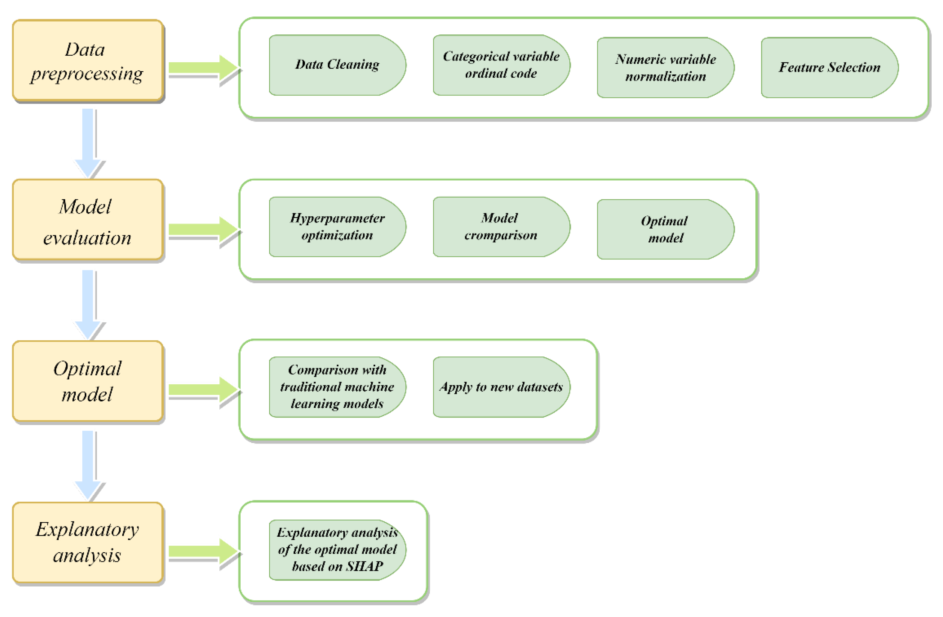
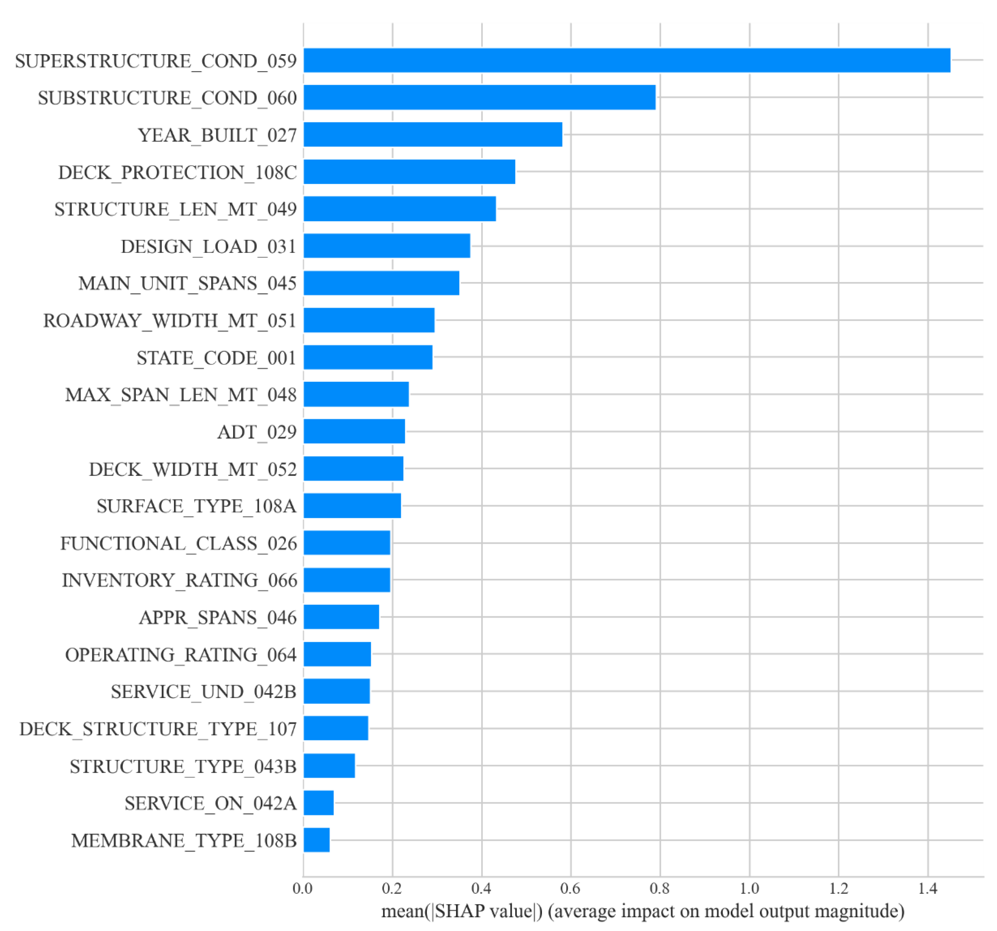
Research on bridge deck condition predictions mainly focuses on bridges with a concrete superstructure and less on bridges with a steel superstructure. Therefore, it is essential to develop a steel bridge deck defect prediction model using an ensemble learning model with good prediction accuracy. In this study, an ensemble-learning-based bridge deck defect prediction model was developed to help bridge managers make more rational and informed steel bridge deck maintenance decisions. This study utilized the latest data from the NBI database for U.S. states for the year 2021 for modeling. It focuses on the following aspects: (1) Addressing the imbalance in the data using the adaptive synthetic sampling method (ADASYN); (2) Six ensemble learning models (RandomForest, ExtraTree, AdaBoost, GBDT, XGBoost, and LightGBM) are established, and the hyperparameters of the models are searched for using the grid search method. The optimal model is determined by comparing the performance evaluation indexes of the six models; (3) The optimal model XGBoost is compared with the traditional machine learning model, and the XGBoost model is applied to the 2019 and 2020 NBI datasets; (4) The interpretable machine learning framework SHAP is used to illustrate the effect of each factor on the condition of the bridge deck defects in the XGBoost model.

2. Methods

2.1. ADASYN

Data imbalance can pose a significant risk to prediction models. The percentage of positive and negative samples in imbalanced data varies greatly; therefore, models trained using these data will favor samples with larger percentages, thus affecting the accuracy of the model [26]. ADASYN is used to generate more data for these harder-to-predict samples with smaller percentages by assigning different weights to the samples with smaller percentages. A more detailed description of ADASYN can be found in the related literature [27].

2.2. RandomForest

Random forest is the most common ensemble learning model. Random forest models use bagging and decision trees as the weak learners during bagging. Random forest models use random sampling, and the selection of samples and each node feature variable in the random forest model is random; thus, the variance of the trained model is small and the generalization ability is strong. Moreover, the random forest model is a parallel operation, and the samples are trained more quickly. The performance of the machine learning model is strongly related to hyperparameter selection; therefore, in order to improve the performance of the model, the hyperparameters need to be optimized. The optimized hyperparameters of the random forest model are described in detail in Section 4.1 [28]. A more detailed description of the random forest model and an explanation of its hyperparameters can be found in the related literature [29].

2.3. ExtraTree

ExtraTree models improve on the random forest model, which uses a random sampling method, whereas ExtraTree models use the full sample for training. Random features and random thresholds are used to select each node feature variable in the ExtraTree model; thus, the randomness of the decision tree in the ExtraTree model will be greater. This reduces overfitting and variance. A more detailed description of the ExtraTree model and an explanation of its hyperparameters can be found in the related literature [30]. The optimized hyperparameters of the ExtraTree model are detailed in Section 4.1.

2.4. AdaBoost

AdaBoost models use boosting and a decision tree model as a weak learner. AdaBoost models first train a weak learner and then assign a weight to each sample and increases the weight of the training samples when the predictions are incorrect. With repeated training, an AdaBoost model can make better predictions for harder samples. A more detailed description of the AdaBoost model and an explanation of its hyperparameters can be found in the related literature [31]. The optimized hyperparameters of the AdaBoost model are detailed in Section 4.1.

2.5. GBDT

GBDT models also use boosting, but use a different iterative approach from the AdaBoost model, which iteratively increases the weight of the predicted error samples, whereas the GBDT model regresses the data using an additive model and continuously decreases the residuals from the training process and uses the negative gradient of the loss function at the value of the current model as an approximation of the residuals in the algorithm. A more detailed description of the GBDT model and an explanation of its hyperparameters can be found in the related literature [32]. The hyperparameters of the optimized GBDT model are detailed in Section 4.1.

2.6. XGBoost

The loss function in the GBDT model is a first-order Taylor expansion, whereas the loss function in the XGBoost model can be a second-order Taylor expansion. The XGBoost model can also reduce overfitting by column sampling. A more detailed description of the XGBoost model and an explanation of its hyperparameters can be found in the related literature [33]. The optimized hyperparameters of the XGBoost model are described in Section 4.1.

2.7. LightGBM

The LightGBM model is a histogram-based gradient boosting framework developed by Microsoft in 2017. The LightGBM model mainly uses two new techniques: gradient-based one-sided sampling (GOSS) and proprietary feature bundling (EFB). Sampling with GOSS allows more attention to be given to samples with large gradients as a way to reduce the impact on computation. Data at higher latitudes are mostly sparse; thus, bundling certain mutually exclusive features together using EFB can reduce the dimensionality of the features. These two new techniques improve the computational speed and accuracy of the LightGBM model. A more detailed description of the LightGBM model and an explanation of its hyperparameters can be found in the related literature [34]. The optimized hyperparameters of the LightGBM model are detailed in Section 4.1.

2.8. SHAP

SHAP is an explanatory analysis method based on the Shapley value in game theory to explain machine learning models, and has become increasingly popular among researchers in recent years for explaining related engineering prediction models. SHAP can be used to determine the degree of influence of each characteristic variable on the prediction results of a model. In addition, SHAP can be used to determine whether each characteristic variable has a positive or negative effect on the results. A more detailed description of SHAP can be found in the related literature [35].

3. Prediction of Steel Bridge Deck Defect Condition Based on Ensemble Learning

The prediction model building process is shown in Figure 1. The main processes are as follows: (1) Processing of the original data; (2) Six ensemble learning models (RandomForest, ExtraTree, AdaBoost, GBDT, XGBoost, and LightGBM) are built using the processed data, and the hyperparameters of the models are optimized. Then, the optimal model is determined by comparing the evaluation metrics of the six models; (3) The optimal models are compared with traditional machine learning models and previous related studies and applied to the new dataset; and (4) An explanatory analysis of the optimal model is performed using SHAP.

3.1. Data Preprocessing

In this study, the latest NBI database data from 2021 were first used to obtain data related to bridges with a steel superstructure material via screening. Then, the data were preprocessed, and the data for the bridges with category N bridge deck conditions (N indicates not applicable) were removed from the dataset followed by eliminating data outliers and missing values to obtain a final dataset containing 139,063 bridges. The condition ratings for the bridge decks in the NBI database are shown in

Table 1. Condition ratings of the bridge decks.

Rating	Description	Target
N	Not applicable.
9	Excellent condition.	Not Defect
8	Very good condition—no problems noted.
7	Good condition—some minor problems.
6	Satisfactory condition—structural elements show some minor deterioration.
5	Fair condition—all primary structural elements are sound but may have minor section loss, cracking, spalling, or scour.
4	Poor condition—advanced section loss, deterioration, spalling, or scour.	Defect
3	Serious condition—section loss, deterioration, spalling, or scour have seriously affected primary structural components. Local failures are possible. Fatigue cracks in steel or shear cracks in concrete may be present.
2	Critical condition—advanced deterioration of primary structural elements. Fatigue cracks in steel or shear cracks in concrete may be present, or scour may have removed substructure support. Unless closely monitored, it may be necessary to close the bridge until corrective action is taken.
1	“Imminent” failure condition—major deterioration or section loss present in critical structural components or obvious vertical or horizontal movement affecting structure stability. The bridge is closed to traffic.
0	Failed condition—out of service—beyond corrective action.

[36].

Based on the deck condition ratings, the steel bridge deck defect condition prediction problem can be viewed as a dichotomous problem (defective and non-defective), with the presence or absence of defects on the steel deck as the target variable. Based on the Federal Highway Administration’s definition of structural defects [37], ratings less than or equal to four were classified as defective conditions, and ratings above four were classified as non-defective conditions. Subsequently, statistical analysis of the target variables in the dataset revealed that there was a sample imbalance in the target variables, in which the proportion of defective samples accounted for 6%. Therefore, this study used ADASYN to process the variable target samples, and the ratio of defective and non-defective samples after processing was 1:1.

The categorical feature variables in the dataset are usually not continuous numbers, and most machine learning algorithms cannot deal with categorical feature variables directly; thus, this paper used a unique thermal coding approach to deal with them. For the numerical feature variables in the dataset, because they possess different magnitudes and magnitudes, data normalization is used to deal with them. The numerical feature variables are transformed into dimensionless, order-of-magnitude difference-normalized values through normalization in order to process the data more efficiently [38].

There are many feature variables in the NBI database, but not all of them are related to the defective condition of the bridge deck; thus, the selection of input feature variables was performed based on previous studies [8,12]. A simple statistical analysis of the individual feature variables is shown in

Table 2. Statistical analysis of characteristic variables.

Variable	Description	Data Type	Variable Type	Mean	Std
STATE_CODE_001	The state code and FHWA region code.	Numeric	Input	30.19	14.16
FUNCTIONAL_CLASS_026	The functional classification of inventory routes.	Categorical	Input	9.64	4.01
YEAR_BUILT_027	The year of bridge construction.	Numeric	Input	1968.27	25.64
ADT_029	The average daily traffic volume.	Numeric	Input	9240.39	22,197.23
DESIGN_LOAD_031	The live load for which the structure was designed.	Categorical	Input	3.44	2.64
SERVICE_ON_042A	Type of service on bridge.	Categorical	Input	1.58	1.47
SERVICE_UND_042B	Type of service under bridge.	Categorical	Input	3.99	1.79
STRUCTURE_TYPE_043B	Type of design and construction.	Numeric	Input	2.52	2.04
MAIN_UNIT_SPANS_045	The number of spans in the main unit.	Numeric	Input	2.45	4.79
APPR_SPANS_046	The number of spans in the approach spans to the major bridge.	Numeric	Input	0.75	10.88
MAX_SPAN_LEN_MT_048	The length of the maximum span.	Numeric	Input	22.31	21.67
STRUCTURE_LEN_MT_049	The length of the structure.	Numeric	Input	69.36	241.82
ROADWAY_WIDTH_MT_051	The most restrictive minimum distance between curbs on the structure roadway.	Numeric	Input	10.01	6.17
DECK_WIDTH_MT_052	The out-to-out width.	Numeric	Input	11.18	7.18
DECK_COND_058	The overall condition rating of the deck	Categorical	Output	0.94	0.22
SUPERSTRUCTURE_COND_059	The physical condition of all structural members of the superstructure	Categorical	Input	6.23	1.18
SUBSTRUCTURE_COND_060	The physical condition of piers, abutments, piles, fenders, footings, etc.	Categorical	Input	6.13	1.17
OPERATING_RATING_064	The absolute maximum permissible load level.	Numeric	Input	51.45	23.26
INVENTORY_RATING_066	The load level that can safely utilize an existing structure	Numeric	Input	32.46	15.83
DECK_STRUCTURE_TYPE_107	The type of deck system.	Categorical	Input	2.14	2.41
SURFACE_TYPE_108A	The type of wearing surface	Categorical	Input	3.37	2.88
MEMBRANE_TYPE_108B	The type of membrane	Categorical	Input	0.73	2.17
DECK_PROTECTION_108C	The type of deck protection.	Categorical	Input	0.82	2.10

. The Pearson correlation coefficient method was then used to explore the correlation between the feature variables in the dataset; the Pearson coefficient correlation matrix is shown in Figure 2. The Pearson correlation coefficient takes values ranging from −1 to 1: when the correlation coefficient is 0, it means that there is no relationship between the two characteristic variables; when the coefficient is closer to 1, it means that the positive correlation between the two characteristic variables is stronger; when the coefficient is closer to −1, it means that the negative correlation between the two characteristic variables is stronger [39]. It can be seen that the selected characteristic variables are correlated with each other; therefore, it is reasonable to use them as characteristic variables in the model.

3.2. Model Building and Evaluation

Before building the machine learning model, it was necessary to divide the dataset into two groups; 70% of the data was used as the training set for model training, and 30% of the data was used as the test set to check how well the final model performed. The selection of hyperparameters for a machine learning model plays an important role in the model’s performance; this study used the network search method to optimize the model’s hyperparameters [28]. The network search method is an exhaustive search method that optimizes the model’s parameters using a 10-fold cross-validation method. The 10-fold cross-validation method divides the dataset into ten mutually exclusive subsets of about the same size by means of stratified sampling, and each training session takes the concatenated set of nine of these subsets as the training set and the remaining one as the test set so that ten different sets of data can be obtained. Using these data for ten training and testing sessions, the final result is the average of the ten training and testing sessions [38]. Using the 10-fold cross-validation method can reduce the overfitting of the model and improve the model’s generalization performance [40].

In order to test whether the model performs well or not, metrics are needed for evaluation. The most commonly used evaluation metrics are accuracy, area under the ROC curve (AUC), precision, recall, and F1-score. These metrics are calculated by the confusion matrix, which is shown in

Table 3. Confusion matrix.

True Value	Predicted Value
	Not Defect	Defect
Not defect	TP	FP
Defect	FN	TN

. True positive (TP) and true negative (TN) denote the number of correct predictions, and false negative (FN) and false positive (FP) denote the number of incorrect predictions. The accuracy rate is defined as the ratio of the number of correctly classified samples to the number of all samples, as shown in Equation (1). The ROC curve reflects the relationship between the true positive rate (TPR) and the false positive rate (FPR), and the AUC is defined as the area enclosed with the coordinate axis under the ROC curve. The closer the AUC value is to 1, the better the model performance is. The true positive rate (TPR) and the false positive rate (FPR) are shown in Equations (2) and (3), respectively. Accuracy and AUC are the overall descriptions of prediction accuracy for all of the samples. Accuracy is defined as the ratio of the number of correctly classified positive samples to the number of classified positive samples, as shown in Equation (4). Recall is defined as the ratio of the number of correctly classified positive samples to the actual number of positive samples, as shown in Equation (5). There is a mutually constraining relationship between precision and recall; thus, the F1-Score should be used as a comprehensive evaluation index [20]. The F1-score is the summed average of precision and recall, as shown in Equation (6), and a higher F1-score is better.

$$\mathrm{Accuracy}=\frac{\mathrm{TP}+\mathrm{TN}}{\mathrm{TP}+\mathrm{FP}+\mathrm{FN}+\mathrm{TN}}$$

(1)

$$\mathrm{TPR}=\frac{\mathrm{TP}}{\mathrm{TP}+\mathrm{FN}}$$

(2)

$$\mathrm{FPR}=\frac{\mathrm{FP}}{\mathrm{FP}+\mathrm{TN}}$$

(3)

$$\mathrm{Precise}=\frac{\mathrm{TP}}{\mathrm{TP}+\mathrm{FP}}$$

(4)

$$\mathrm{Recall}=\frac{\mathrm{TP}}{\mathrm{TP}+\mathrm{FN}}$$

(5)

$$\mathrm{F}1-\mathrm{score}=2\times \frac{\mathrm{Precise}\times \mathrm{Recall}}{\mathrm{Precise}+\mathrm{Recall}}$$

(6)

4. Results and Discussion

4.1. Hyperparameter Optimization

The grid search method was used to optimize the hyperparameters of the developed ensemble learning model by first determining a range of values for each hyperparameter of the model and then generating multiple hyperparameter combinations. Next, these hyperparameter combinations were applied to the model and evaluated by 10-fold cross-validation on the training set. Finally, the mean value of the ten evaluations of each hyperparameter combination was compared, determining the optimal combination. In this study, accuracy was chosen as the main evaluation metric for hyperparameter optimization to select the hyperparameter combination with the best performance.

The optimal hyperparameter combination in the RandomForest model is bootstrap = True; n_estimators = 100; criterion = ‘gini’; min_samples_leaf = 1; min_samples_split = 2. The optimal hyperparameter combination corresponds to 10-fold crossover. The validation results are shown in

Table 4. The 10-fold cross-validation results for RandomForest.

	Evaluation Metrics
	Accuracy	AUC	Recall	Precision	F1-Score
1	0.9457	0.8950	0.9791	0.9641	0.9715
2	0.9447	0.9027	0.9753	0.9667	0.9710
3	0.9468	0.8916	0.9786	0.9657	0.9721
4	0.9459	0.8955	0.9772	0.9660	0.9716
5	0.9425	0.8756	0.9775	0.9624	0.9699
6	0.9439	0.8902	0.9781	0.9633	0.9706
7	0.9431	0.8869	0.9767	0.9637	0.9702
8	0.9442	0.8967	0.9755	0.9660	0.9707
9	0.9436	0.9032	0.9756	0.9652	0.9704
10	0.9425	0.8904	0.9761	0.9636	0.9698
Mean	0.9443	0.8928	0.9770	0.9647	0.9708
SD	0.0014	0.0076	0.0013	0.0013	0.0007

.

The optimal hyperparameter combinations in the Extra Tree model are bootstrap = False; n_estimators = 100; criterion = ‘gini’; min_samples_leaf = 1; and min_samples_split = 2. The optimal hyperparameter combinations correspond to 10-fold cross-validation results shown in

Table 5. The 10-fold cross-validation results for ExtraTree.

	Evaluation Metrics
	Accuracy	AUC	Recall	Precision	F1-Score
1	0.9431	0.8794	0.9762	0.9642	0.9702
2	0.9441	0.8976	0.9766	0.9649	0.9707
3	0.9437	0.8732	0.9764	0.9647	0.9705
4	0.9459	0.8750	0.9789	0.9645	0.9716
5	0.9410	0.8619	0.9764	0.9620	0.9691
6	0.9403	0.8772	0.9765	0.9612	0.9688
7	0.9436	0.8800	0.9785	0.9626	0.9705
8	0.9429	0.8797	0.9752	0.9649	0.9700
9	0.9415	0.8871	0.9760	0.9628	0.9694
10	0.9388	0.8709	0.9724	0.9634	0.9678
Mean	0.9425	0.8782	0.9763	0.9635	0.9699
SD	0.0020	0.0091	0.0017	0.0013	0.0010

.

The optimal hyperparameter combination in the AdaBoost model is algorithm = ‘SAMME.R’; Learning rate = 0.2; n_estimators = 200. The results of the 10-fold cross-validation corresponding to the optimal hyperparameter combination are shown in

Table 6. The 10-fold cross-validation results for AdaBoost.

	Evaluation Metrics
	Accuracy	AUC	Recall	Precision	F1-Score
1	0.8273	0.8693	0.8314	0.9838	0.9012
2	0.8269	0.8925	0.8296	0.9854	0.9008
3	0.8134	0.8739	0.8171	0.9830	0.8924
4	0.8193	0.8714	0.8231	0.9835	0.8962
5	0.8236	0.8579	0.8302	0.9807	0.8992
6	0.8238	0.8674	0.8291	0.9823	0.8992
7	0.8147	0.8609	0.8195	0.9819	0.8934
8	0.8248	0.8772	0.8273	0.9855	0.8995
9	0.8238	0.8769	0.8274	0.9841	0.8990
10	0.8196	0.8726	0.8234	0.9836	0.8964
Mean	0.8217	0.8720	0.8258	0.9834	0.8977
SD	0.0046	0.0091	0.0046	0.0014	0.0029

.

The optimal hyperparameter combinations in the GBDT model are learning_rate = 0.15; max_depth = 10; n_estimators = 210; min_samples_leaf = 3; min_samples_split = 7. The optimal hyperparameter combinations correspond to the 10-fold cross-validation results shown in

Table 7. The 10-fold cross-validation results for GBDT.

	Evaluation Metrics
	Accuracy	AUC	Recall	Precision	F1-Score
1	0.9483	0.8882	0.9834	0.9629	0.9730
2	0.9486	0.9087	0.9825	0.9639	0.9732
3	0.9489	0.8918	0.9832	0.9637	0.9733
4	0.9466	0.8850	0.9814	0.9630	0.9721
5	0.9437	0.8696	0.9817	0.9598	0.9706
6	0.9445	0.8769	0.9822	0.9602	0.9711
7	0.9469	0.8809	0.9835	0.9613	0.9723
8	0.9493	0.8914	0.9829	0.9643	0.9735
9	0.9467	0.8957	0.9814	0.9631	0.9721
10	0.9454	0.8831	0.9810	0.9621	0.9715
Mean	0.9469	0.8871	0.9823	0.9624	0.9723
SD	0.0018	0.0103	0.0009	0.0015	0.0009

.

The optimal hyperparameter combination in the XGBoost model is base_score = 0.5; boosters = ‘gbtree’; colsample_bylevel = 1; colsample_bynode = 1; colsample_bytree = 0.5; gamma = 0; learning_rate = 0.1; max_depth = 11; min_child_weight = 1; n_estimators = 260; objective = ‘binary: logistic’; reg_alpha = 0.05; reg_lambda = 0.3. The optimal hyperparameter combinations correspond to the 10-fold cross-validation results shown in

Table 8. The 10-fold cross-validation results for XGBoost.

	Evaluation Metrics
	Accuracy	AUC	Recall	Precision	F1-Score
1	0.9514	0.9053	0.9996	0.9516	0.9750
2	0.9503	0.9154	0.9995	0.9506	0.9744
3	0.9512	0.9002	0.9993	0.9516	0.9749
4	0.9526	0.8989	0.9997	0.9527	0.9756
5	0.9509	0.8837	0.9997	0.9510	0.9747
6	0.9508	0.8920	0.9993	0.9512	0.9747
7	0.9509	0.8927	0.9997	0.9510	0.9747
8	0.9518	0.9035	0.9995	0.9521	0.9752
9	0.9503	0.9022	0.9996	0.9505	0.9744
10	0.9509	0.8980	0.9998	0.9509	0.9747
Mean	0.9511	0.8992	0.9996	0.9513	0.9748
SD	0.0007	0.0082	0.0001	0.0006	0.0003

.

The optimal combination of hyperparameters in the LightGBM model is bagging_fraction = 0.9; bagging_freq = 4; boosting_type = ‘gbdt’; colsample_bytree = 1.0; feature_fraction = 0.4; importance_type = ‘split’; learning_rate = 0.5; min_child_samples = 71; min_child_weight = 0.001; min_split_gain = 0.4; n_estimators = 280; num_leaves = 6; reg_alpha = 1; reg_lambda = 0.7. The optimal hyperparameter combinations correspond to the 10-fold cross-validation results shown in

Table 9. The 10-fold cross-validation results for LightGBM.

	Evaluation Metrics
	Accuracy	AUC	Recall	Precision	F1-Score
1	0.9479	0.8946	0.9846	0.9614	0.9728
2	0.9487	0.9112	0.9857	0.9612	0.9733
3	0.9507	0.8880	0.9855	0.9633	0.9743
4	0.9475	0.8894	0.9831	0.9623	0.9726
5	0.9474	0.8690	0.9857	0.9599	0.9726
6	0.9463	0.8850	0.9854	0.9591	0.9720
7	0.9480	0.8850	0.9851	0.9610	0.9729
8	0.9481	0.8925	0.9838	0.9623	0.9729
9	0.9470	0.8974	0.9831	0.9618	0.9723
10	0.9454	0.8905	0.9833	0.9601	0.9716
Mean	0.9477	0.8902	0.9845	0.9612	0.9727
SD	0.0013	0.0101	0.0010	0.0012	0.0007

.

The mean values of the 10-fold cross-validation results corresponding to the optimal hyperparameter combinations of the six ensemble learning models on the training set are shown in Figure 3. From the figure, it can be seen that the XGBoost model has the best performance on the training set, and the AdaBoost model has the worst results.

4.2. Model Comparison

In order to validate and evaluate the performance of the developed models, the trained models were validated on the test set, and the evaluation metrics of the six developed ensemble learning models on the test set are shown in

Table 10. Evaluation results on the ensemble learning model test set.

Model	Evaluation Metrics
	Accuracy	AUC	Recall	Precision	F1-Score
RandomForest	0.9446	0.8999	0.9772	0.9647	0.9709
ExtraTree	0.9431	0.8881	0.9765	0.9638	0.9701
AdaBoost	0.8220	0.8768	0.8252	0.9841	0.8977
GBDT	0.9471	0.8902	0.9835	0.9615	0.9724
XGBoost	0.9495	0.9026	0.9994	0.9498	0.9740
LightGBM	0.9459	0.8928	0.9833	0.9605	0.9717

. The evaluation metrics for each model on the test set are compared with the evaluation metrics on the training set. The values are close to each other, indicating that no overfitting occurs in these models. It can be seen from Figure 4 that the XGBoost model has the highest accuracy, AUC, and F1-score on the test set; therefore, the XGBoost model is the best prediction model among the six ensemble learning models.

4.3. Best Model

According to Section 4.2, the best-performing model among the established ensemble learning models is XGBoost. To better reflect the superiority of ensemble learning models, this paper compares the XGBoost model with other traditional machine learning models. The most widely applied K-nearest neighbor (KNN) and support vector machine (SVM) models were chosen.

Table 11. XGBoost model versus traditional machine learning models.

Model	Evaluation Metrics
	Accuracy	AUC	Recall	Precision	F1-Score
XGBoost	0.9495	0.9026	0.9994	0.9498	0.9740
KNN	0.8451	0.8063	0.8561	0.9774	0.9127
SVM	0.7590	0.7976	0.7543	0.9881	0.8555

shows the evaluation results of the KNN and SVM models on the test set, and it can be seen that the XGBoost model performed well. The XGBoost model was compared with the KNN model and showed a 13% improvement in accuracy, a 12% improvement in the AUC, and a 7% improvement in the F1-score. The XGBoost model was compared with the SVM model and showed a 25% improvement in accuracy, the AUC improved by 13%, and the F1-score improved by 14%. Collectively, it seems that the ensemble learning model demonstrates significant performance improvements over the traditional machine learning models used for steel bridge deck defect condition prediction problems. In addition, the XGBoost model developed in this study was compared with the results of previous related studies, and the comparison results are shown in

Table 12. Comparison of XGBoost model with models from related studies.

Model	Evaluation Metrics
XGBoost	0.95
ANN [8]	0.92
ANN [16]	0.75

, from which it can be seen that the model developed in this study performed well.

In this study, to further test the performance of the best model, the trained model was applied to a new dataset to explore the generalization performance. The data from the 2020 and 2019 NBI databases were first processed as in Section 3.1 and then predicted using the trained XGBoost model in this study; the results are shown in

Table 13. XGBoost model performance on the new dataset.

Dataset	Accuracy
NBI-2020	0.9526
NBI-2019	0.9505

. As shown in Table 13, the XGBoost model achieved good accuracy on both new datasets, indicating that the established XGBoost model has good generalization performance. In summary, the XGBoost model developed in this study can be used as an accurate method to predict the condition of steel bridge deck defects.

4.4. Explanation of the Best Model

Machine learning models mostly lack interpretability; thus, this study used SHAP architecture to study the sensitivity of each input feature variable to the target feature variable to obtain the importance of each input feature variable. The importance of the input feature variables of the XGBoost model was analyzed using the SHAP architecture, and the importance of the input feature variables is shown in Figure 5. The most important feature variable is the condition of the bridge superstructure. The feature variables that are relatively more important are the bridge substructure condition and the year of bridge construction, as seen in Figure 5. The x-axis of the SHAP feature dependence diagram represents the feature value. The y-axis represents the SHAP value corresponding to the feature value. A higher positive SHAP value indicates a higher probability of the steel bridge deck condition being classified as being in a non-defective condition. A higher negative SHAP value indicates a higher probability of being classified as having a defective condition.

Figure 6 shows the characteristic dependence of the bridge superstructure condition, and it can be seen that the higher the bridge superstructure condition level, the higher the SHAP value, which indicates that the bridge superstructure condition better, and it is less likely that the bridge deck has defects. This is because the steel bridge deck and the superstructure share the vehicle load; thus, the condition of the steel bridge deck is more susceptible to the influence of the superstructure. Figure 7 shows the characteristic dependence of the bridge substructure condition, which shows that the better the substructure condition, the less likely the bridge deck is to be defective. Figure 8 shows the characteristic dependence of the bridge construction year. It can be seen that the SHAP value became larger as the construction year becomes closer, which indicates that the more recent the construction, the less likely the deck is to have defects; therefore, bridge managers should pay more attention to older steel bridge decks.

5. Conclusions

This study developed an ensemble-learning-based steel bridge deck defect condition prediction model that can help bridge managers make more rational and informed decisions regarding steel bridge deck maintenance. This study explored steel bridge deck defect condition predictions as a dichotomous problem, using the latest data from the NBI database for 2021. The data were first pre-processed, and imbalances in the data were solved using ADASYN. Then, six ensemble learning models (RandomForest, ExtraTree, AdaBoost, GBDT, XGBoost, and LightGBM) were built, the hyperparameters of the models were optimized, and the performance of the six ensemble learning models was compared with determine the optimal prediction model. Next, to demonstrate the superiority of the optimal model performance, the optimal model was compared with traditional machine learning models and previous related studies, and the optimal model was applied to a new dataset. Finally, an explanatory analysis of the optimal model was performed using the SHAP framework. The following conclusions can be drawn from the study:

(1)

The optimal hyperparameters of the models were determined using the grid search method, and the optimal hyperparameter combinations of six ensemble learning models were obtained.

(2)

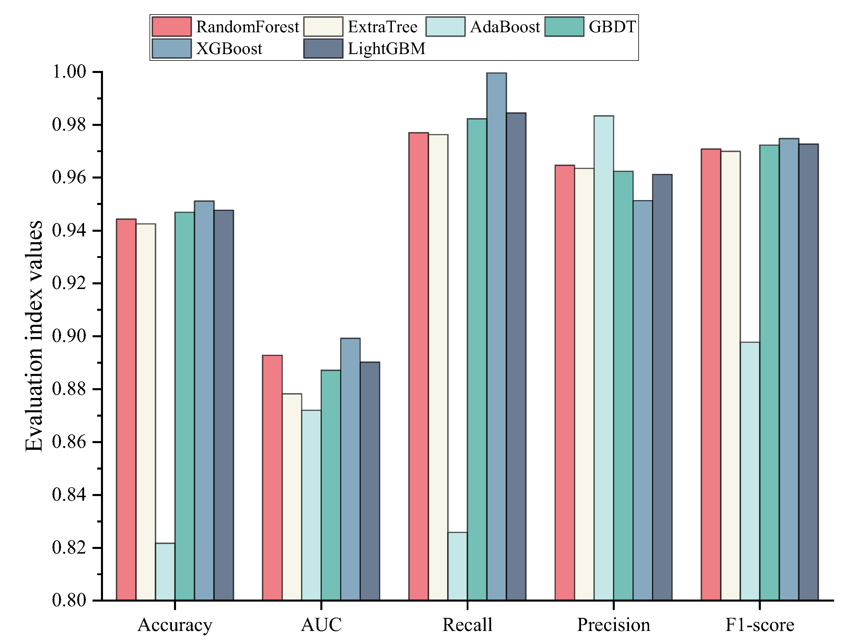
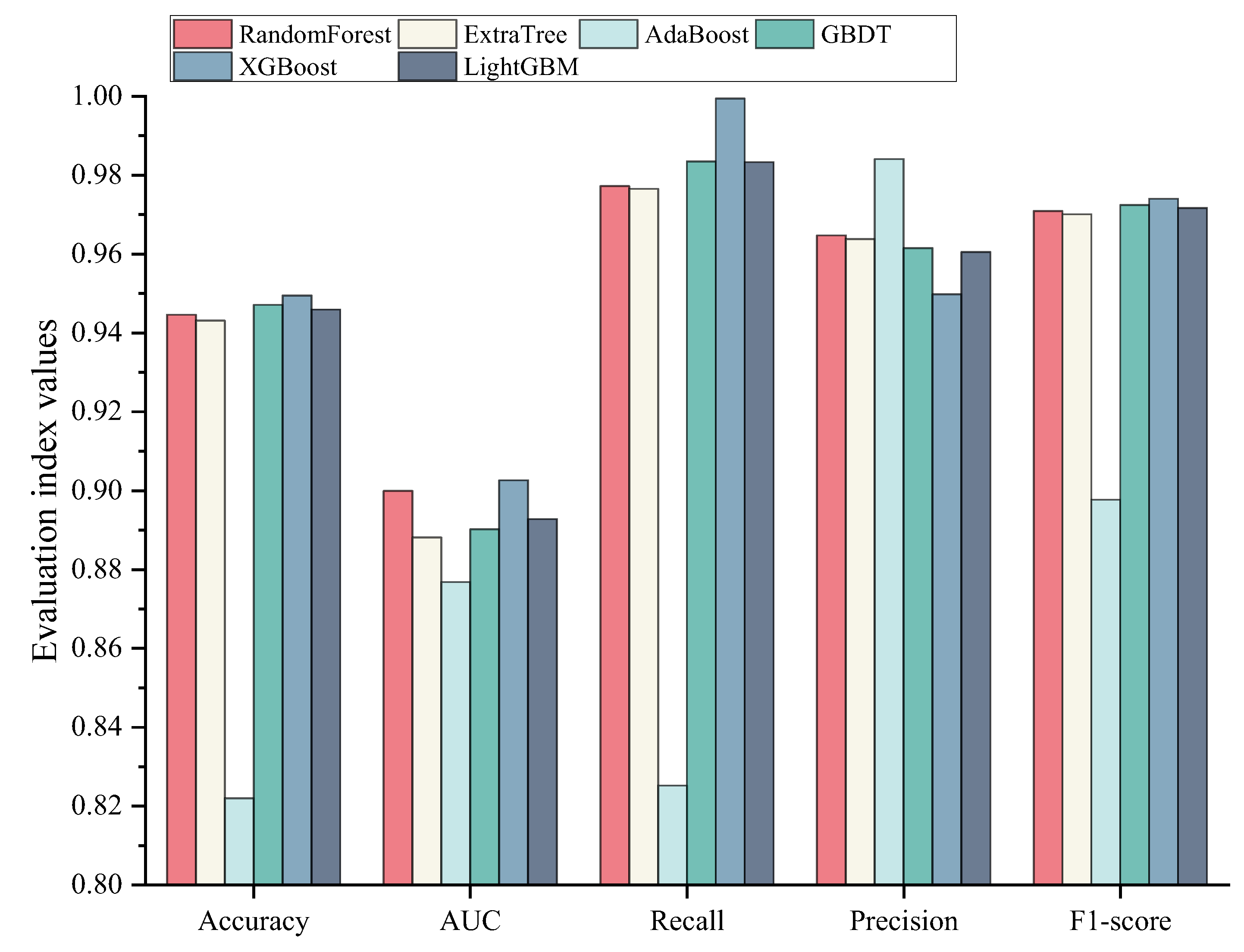
The optimal prediction model is XGBoost, with a model accuracy of 0.9495, an AUC of 0.9026, and an F1-Score of 0.9740. The performance of the model is improved compared with traditional machine learning models, and the comparison with previous studies also demonstrated the superiority of the model’s performance. The XGBoost model also performed well on the 2019 and 2020 NBI datasets, showing that the model has good generalization performance, indicating that the model has good generalization performance. Therefore, the XGBoost model developed in this study can be used as an accurate method to predict the condition of steel bridge deck defects.

(3)

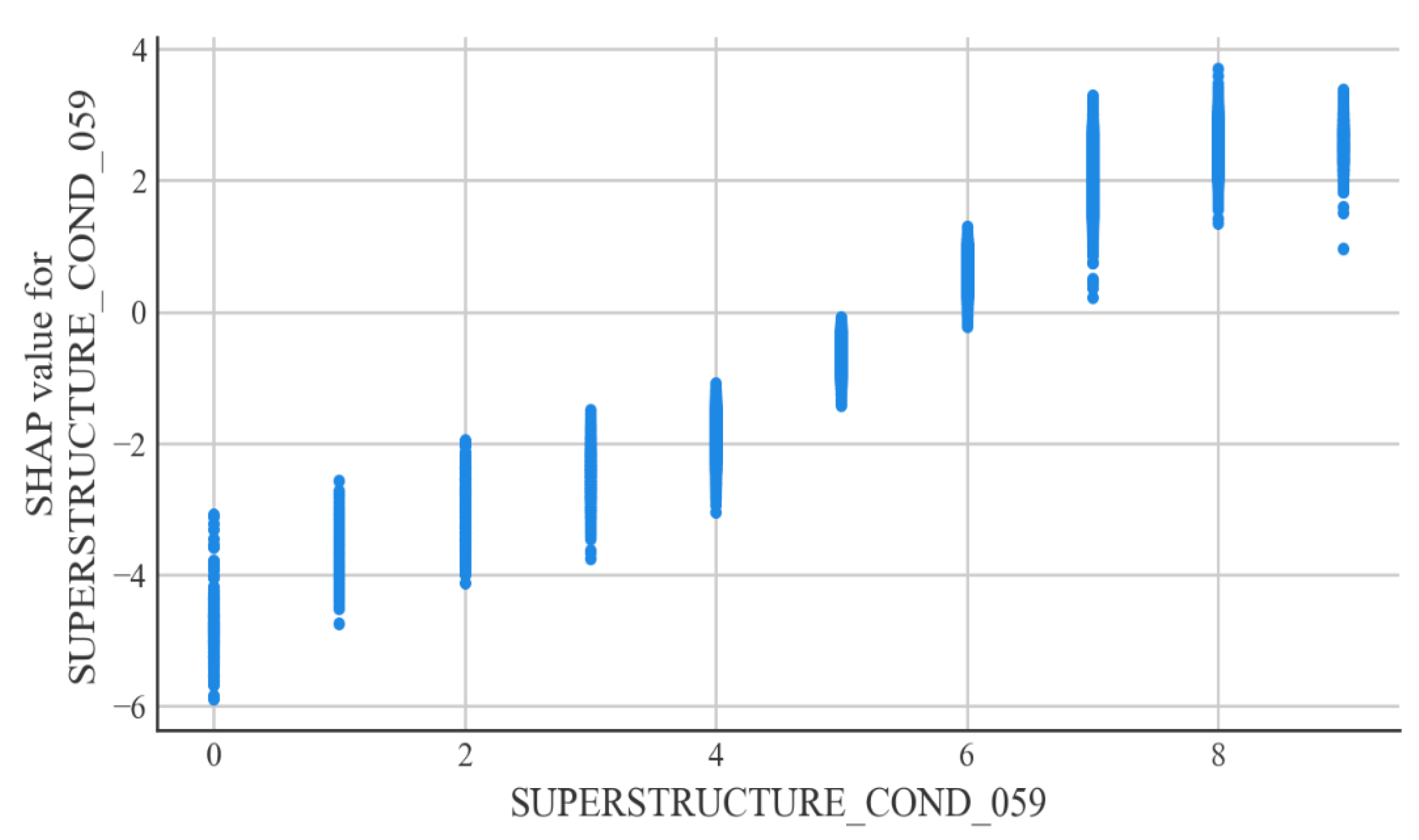
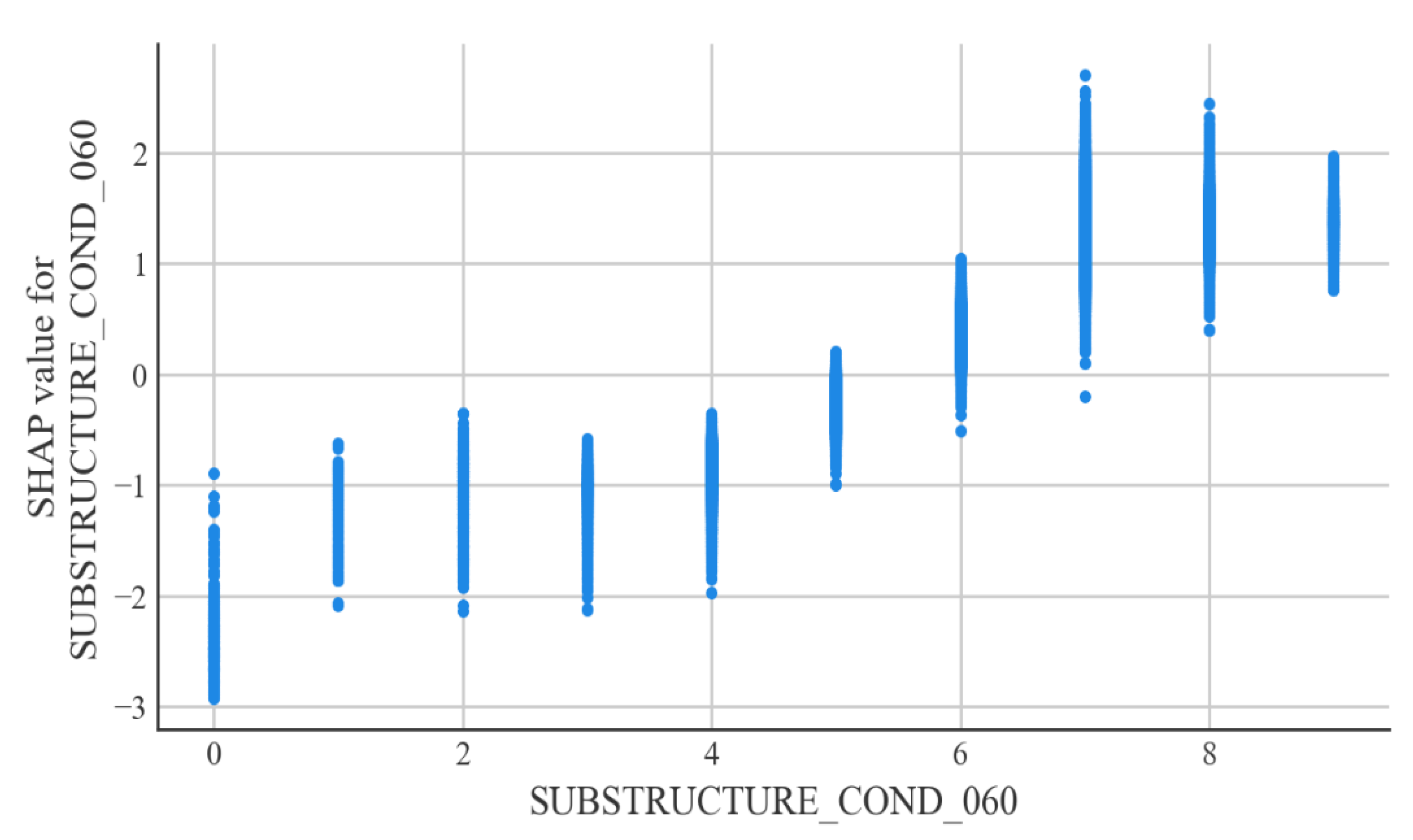
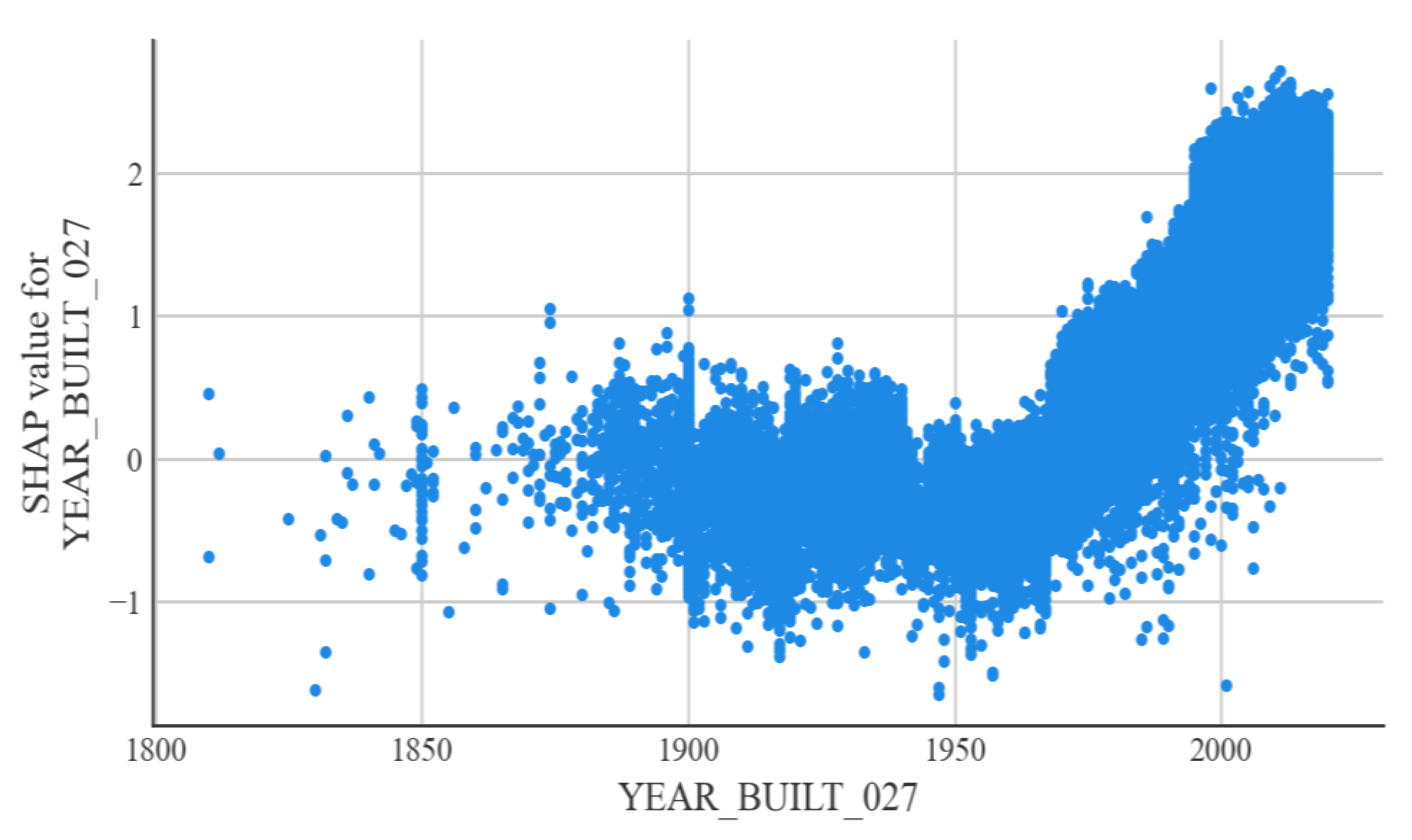
According to the interpretable machine learning framework SHAP, the most important factor affecting the condition of steel bridge deck defects is the condition of the bridge superstructure. Relatively minor factors are the condition of the bridge substructure and the year of bridge construction. The better the condition of the superstructure and substructure of a steel bridge, the less likely the bridge deck is to be defective. The older the steel bridge deck is, the more likely it is that it will have defects. The explanatory analysis of the model is consistent with the actual situation in engineering applications and can justify the developed model.

The ensemble learning model developed using this study can help bridge managers to accurately predict the condition of steel bridge deck defects. Additionally, based on the important factors affecting the condition of steel bridge decks obtained in this study, bridge managers should prioritize the maintenance of each steel bridge component when making maintenance decisions and ensure the rational use of funds. Steel bridges have a lot of room for development in China, and as the number of steel bridges in China rises, it is important to establish a database of the steel bridges in China. The future use of the Chinese steel bridge database to build a bridge deck condition prediction model will be more beneficial for Chinese bridge managers in making steel bridge deck maintenance decisions.

Contemporary assessments of bridge defects are usually carried out by manual inspection methods, which are highly subjective [41]. To solve this problem, sensor-based detection methods and computer-vision-based detection methods can also be used to obtain bridge assessment data [42]. The models developed in this study can also be used in conjunction with these detection techniques.

References

1. Lu, Q.; Bors, J. Alternate uses of epoxy asphalt on bridge decks and roadways. Constr. Build. Mater. 2015, 78, 18–25. [Google Scholar] [CrossRef]
2. Liu, C.; Qian, Z.; Liao, Y.; Ren, H. A Comprehensive Life-Cycle Cost Analysis Approach Developed for Steel Bridge Deck Pavement Schemes. Coatings 2021, 11, 565. [Google Scholar] [CrossRef]
3. Luo, S.; Qian, Z.; Yang, X.; Lu, Q. Laboratory evaluation of double-layered pavement structures for long-span steel bridge decks. J. Mater. Civ. Eng. 2018, 30, 04018111. [Google Scholar] [CrossRef]
4. Chen, X.; Huang, W.; Qian, Z.; Zhang, L. Design principle of deck pavements for long-span steel bridges with heavy-duty traffic in China. Road Mater. Pavement Des. 2017, 18 (Suppl. 3), 226–239. [Google Scholar] [CrossRef]
5. Chen, X.; Qian, Z.; Liu, X.; Lei, Z. State of the art of asphalt surfacings on long-spanned orthotropic steel decks in China. J. Test. Eval. 2012, 40, 1252–1259. [Google Scholar] [CrossRef] [Green Version]
6. Fereshtehnejad, E.; Gazzola, G.; Parekh, P.; Nakrani, C.; Parvardeh, H. Detecting Anomalies in National Bridge Inventory Databases Using Machine Learning Methods. Transp. Res. Rec. 2022, 03611981221075028. [Google Scholar] [CrossRef]
7. Nasrollahi, M.; Washer, G. Estimating inspection intervals for bridges based on statistical analysis of national bridge inventory data. J. Bridge Eng. 2015, 20, 04014104. [Google Scholar] [CrossRef]
8. Assaad, R.; El-adaway, I.H. Bridge infrastructure asset management system: Comparative computational machine learning approach for evaluating and predicting deck deterioration conditions. J. Infrastruct. Syst. 2020, 26, 04020032. [Google Scholar] [CrossRef]
9. Dorafshan, S.; Azari, H. Deep learning models for bridge deck evaluation using impact echo. Constr. Build. Mater. 2020, 263, 120109. [Google Scholar] [CrossRef]
10. Pedneault, J.; Desjardins, V.; Margni, M.; Conciatori, D.; Fafard, M.; Sorelli, L. Economic and environmental life cycle assessment of a short-span aluminium composite bridge deck in Canada. J. Clean. Prod. 2021, 310, 127405. [Google Scholar] [CrossRef]
11. Wang, C.; Yao, C.; Zhao, S.; Zhao, S.; Li, Y. A Comparative Study of a Fully-Connected Artificial Neural Network and a Convolutional Neural Network in Predicting Bridge Maintenance Costs. Appl. Sci. 2022, 12, 3595. [Google Scholar] [CrossRef]
12. Ghonima, O.; Anderson, J.C.; Schumacher, T.; Unnikrishnan, A. Performance of US concrete highway bridge decks characterized by random parameters binary logistic regression. ASCE-ASME J. Risk Uncertain. Eng. Syst. Part A: Civ. Eng. 2020, 6, 04019025. [Google Scholar] [CrossRef]
13. Lavrenz, S.M.; Saeed, T.U.; Murillo-Hoyos, J.; Volovski, M.; Labi, S. Can interdependency considerations enhance forecasts of bridge infrastructure condition? Evidence using a multivariate regression approach. Struct. Infrastruct. Eng. 2020, 16, 1177–1185. [Google Scholar] [CrossRef]
14. Ranjith, S.; Setunge, S.; Gravina, R.; Venkatesan, S. Deterioration prediction of timber bridge elements using the Markov chain. J. Perform. Constr. Facil. 2013, 27, 319–325. [Google Scholar] [CrossRef]
15. Mohammed Abdelkader, E.; Zayed, T.; Marzouk, M. A computerized hybrid Bayesian-based approach for modelling the deterioration of concrete bridge decks. Struct. Infrastruct. Eng. 2019, 15, 1178–1199. [Google Scholar] [CrossRef]
16. Huang, Y.-H. Artificial neural network model of bridge deterioration. J. Perform. Constr. Facil. 2010, 24, 597–602. [Google Scholar] [CrossRef]
17. Contreras-Nieto, C.; Shan, Y.; Lewis, P. Characterization of steel bridge superstructure deterioration through data mining techniques. J. Perform. Constr. Facil. 2018, 32, 04018062. [Google Scholar] [CrossRef]
18. Liu, H.; Zhang, Y. Bridge condition rating data modeling using deep learning algorithm. Struct. Infrastruct. Eng. 2020, 16, 1447–1460. [Google Scholar] [CrossRef]
19. Li, Q.-F.; Song, Z.-M. High-performance concrete strength prediction based on ensemble learning. Constr. Build. Mater. 2022, 324, 126694. [Google Scholar] [CrossRef]
20. Zhou, Z.-H. Ensemble Methods: Foundations and Algorithms; Chapman and Hall/CRC: London, UK, 2019. [Google Scholar]
21. Chen, S.-Z.; Feng, D.-C.; Han, W.-S.; Wu, G. Development of data-driven prediction model for CFRP-steel bond strength by implementing ensemble learning algorithms. Constr. Build. Mater. 2021, 303, 124470. [Google Scholar] [CrossRef]
22. Farooq, F.; Ahmed, W.; Akbar, A.; Aslam, F.; Alyousef, R. Predictive modeling for sustainable high-performance concrete from industrial wastes: A comparison and optimization of models using ensemble learners. J. Clean. Prod. 2021, 292, 126032. [Google Scholar] [CrossRef]
23. Chen, W.; Zhang, L. Building vulnerability assessment in seismic areas using ensemble learning: A Nepal case study. J. Clean. Prod. 2022, 350, 131418. [Google Scholar] [CrossRef]
24. Gong, H.; Sun, Y.; Hu, W.; Polaczyk, P.A.; Huang, B. Investigating impacts of asphalt mixture properties on pavement performance using LTPP data through random forests. Constr. Build. Mater. 2019, 204, 203–212. [Google Scholar] [CrossRef]
25. Liang, W.; Luo, S.; Zhao, G.; Wu, H. Predicting hard rock pillar stability using GBDT, XGBoost, and LightGBM algorithms. Mathematics 2020, 8, 765. [Google Scholar] [CrossRef]
26. Brown, I.; Mues, C. An experimental comparison of classification algorithms for imbalanced credit scoring data sets. Expert Syst. Appl. 2012, 39, 3446–3453. [Google Scholar] [CrossRef] [Green Version]
27. He, H.; Bai, Y.; Garcia, E.A.; Li, S. In ADASYN: Adaptive synthetic sampling approach for imbalanced learning. In Proceedings of the 2008 IEEE International Joint Conference on Neural Networks (IEEE World Congress on Computational Intelligence), Hong Kong, 1–8 June 2008; IEEE: Piscataway, NJ, USA, 2008; pp. 1322–1328. [Google Scholar]
28. Zhang, C.; Liu, C.; Zhang, X.; Almpanidis, G. An up-to-date comparison of state-of-the-art classification algorithms. Expert Syst. Appl. 2017, 82, 128–150. [Google Scholar] [CrossRef]
29. Genuer, R.; Poggi, J.-M. Random forests. In Random Forests with R; Springer: Berlin/Heidelberg, Germany, 2020; pp. 33–55. [Google Scholar]
30. Geurts, P.; Ernst, D.; Wehenkel, L. Extremely randomized trees. Mach. Learn. 2006, 63, 3–42. [Google Scholar] [CrossRef] [Green Version]
31. Ying, C.; Qi-Guang, M.; Jia-Chen, L.; Lin, G. Advance and prospects of AdaBoost algorithm. Acta Autom. Sin. 2013, 39, 745–758. [Google Scholar]
32. Hastie, T.; Tibshirani, R.; Friedman, J.H.; Friedman, J.H. The Elements of Statistical Learning: Data Mining, Inference, and Prediction; Springer: Berlin/Heidelberg, Germany, 2009; Volume 2. [Google Scholar]
33. Chen, T.; Guestrin, C. Xgboost: A scalable tree boosting system. In Proceedings of the 22nd ACM SIGKDD International Conference on Knowledge Discovery and Data Mining, San Francisco, CA, USA, 13–17 August 2016; pp. 785–794. [Google Scholar]
34. Ke, G.; Meng, Q.; Finley, T.; Wang, T.; Chen, W.; Ma, W.; Ye, Q.; Liu, T.-Y. Lightgbm: A highly efficient gradient boosting decision tree. Adv. Neural Inf. Processing Syst. 2017, 30. Available online: https://papers.nips.cc/paper/2017/hash/6449f44a102fde848669bdd9eb6b76fa-Abstract.html (accessed on 6 April 2022).
35. Lundberg, S.M.; Lee, S.-I. A unified approach to interpreting model predictions. Adv. Neural Inf. Processing Syst. 2017, 30. Available online: https://arxiv.org/abs/1705.07874 (accessed on 6 April 2022).
36. Administration, F.H. Recording and Coding Guide for the Structure Inventory and Appraisal of the Nation’s Bridges; US Department of Transportation: Washington, DC, USA, 1995. [Google Scholar]
37. Administration, F.H. National Performance Management Measures; Assessing Pavement Condition for the National Highway Performance Program and Bridge Condition for the National Highway Performance Program. Fed. Regist. 2017, 82, 14438–14439. [Google Scholar]
38. Pedregosa, F.; Varoquaux, G.; Gramfort, A.; Michel, V.; Thirion, B.; Grisel, O.; Blondel, M.; Prettenhofer, P.; Weiss, R.; Dubourg, V. Scikit-learn: Machine learning in Python. J. Mach. Learn. Res. 2011, 12, 2825–2830. [Google Scholar]
39. Mohri, M.; Rostamizadeh, A.; Talwalkar, A. Foundations of Machine Learning; MIT Press: Cambridge, MA, USA, 2018. [Google Scholar]
40. Fernández-Delgado, M.; Cernadas, E.; Barro, S.; Amorim, D. Do we need hundreds of classifiers to solve real world classification problems? J. Mach. Learn. Res. 2014, 15, 3133–3181. [Google Scholar]
41. Hadjidemetriou, G.M.; Herrera, M.; Parlikad, A.K. Condition and criticality-based predictive maintenance prioritisation for networks of bridges. Struct. Infrastruct. Eng. 2021, 1–16. [Google Scholar] [CrossRef]
42. Santarsiero, G.; Masi, A.; Picciano, V.; Digrisolo, A. The Italian guidelines on risk classification and management of bridges: Applications and remarks on large scale risk assessments. Infrastructures 2021, 6, 111. [Google Scholar] [CrossRef]
Figure 1. Predictive model flow chart.
Applsci 12 05442 g001
Figure 2. Pearson coefficient correlation matrix.
Applsci 12 05442 g002
Figure 3. Evaluation results of the ensemble learning models on the training set.
Applsci 12 05442 g003
Figure 4. Evaluation results of the ensemble learning models on the test set.
Applsci 12 05442 g004
Figure 5. Importance of input feature variables.
Applsci 12 05442 g005
Figure 6. Bridge superstructure condition characteristics dependence diagram.
Applsci 12 05442 g006
Figure 7. Bridge substructure condition characteristics dependence diagram.
Applsci 12 05442 g007
Figure 8. Bridge construction year characteristics dependency chart.
Applsci 12 05442 g008