Hybrid Deep Neural Network Model for Multi-Step Energy Prediction of Prosumers

Abstract

The transition toward decentralized renewable energy transforms the energy grid, with the prosumers playing an active role in the local energy management. Accurate day-ahead prediction of their energy demand is a prerequisite to ensure the stability and efficiency of the power grid by balancing the energy demand with the production, while incorporating renewable energy as much as possible. In this paper, we propose a 24-steps-ahead energy prediction model that integrates clustering and multilayer perceptron classification models used to detect the classes of energy profiles and multilayer perceptron regression models used to fine-tune the energy prediction, considering the energy data streams. We introduce new features derived from the raw energy data collected from prosumers, such as the profile peaks and valleys, concerning the energy baseline and describe a software infrastructure for integrating the real-time energy data streams with the hybrid deep learning models training and prediction. The evaluation tests consider energy datasets that are closer to the real-time energy data streams from prosumers. The results show that, even on energy data streams, the model offers a good prediction accuracy for small- and medium-scale prosumers.

1. Introduction

Lately, there has been a considerable increase in interest in developing automated power grid management and distribution systems. The transition toward decentralized renewable energy makes energy grid management rather complicated and exposed to uncertainty. The stochastic nature of renewable energy and high variability in the energy demand of small and medium-scale consumers makes it difficult to correlate the increasing energy demand and energy availability at the edge of the grid. Moreover, with the adoption of small-scale renewable energy, the consumers of energy are transformed into prosumers that can play an active role in the management of the smart grid [1]. To better plan the available energy sources, the energy grid management processes are relying on the short-term prediction of energy demand, production, or flexibility. Accurate energy prediction catalyzes the transformation of prosumers into active energy players into smart grids [2]. They can contribute to the stability and efficiency of the power grid by balancing the energy demand with the production in demand response programs, while incorporating, at a larger extent, renewable energy.

There are many use cases related to energy trading, management, and optimization of microgrids or hybrid energy storage that require accurate predictions of energy or price with different time granularities and forecast horizons. Energy prediction is necessary to address problems related to optimal energy management, safety in distribution, and losses reduction. The energy consumption and production of a microgrid must be estimated in advance to better plan the available energy resources or storage usage. In the case of energy trading, the prediction of energy price helps in minimizing the energy costs or increasing the profit of energy prosumers [3,4]. Energy forecasting engines integrated with grid controllers are studied for better energy management [5,6,7]. The prediction of price-based demand–response signal and energy consumption patterns are integrated with home energy management controllers to increase energy efficiency and reduce electricity bills. The optimal power flow strategies could be implemented by using model-based predictive control [8]. The prediction models can be extended to the integration of other flavors of energy, such as the thermal energy or water distribution [9,10], and are useful in detecting abnormal behavior in energy consumption [11].

The significant increase in computing power and the evolution areas, such as the Internet of Things (IoT), Big Data, and Machine Learning, facilitate the development of intelligent management and control of energy systems [12,13]. Smart energy meters or sensors can be easily installed in key points of the grid or at prosumers to monitor and collect relevant information for the management processes. They provide a constant flow of data to be used by intelligent systems in the prediction processes and to take decisions to enforce the security, safety, stability, and performance of the smart grid.

The challenge is that the huge amount of energy data generated by all these measuring instruments must be collected and processed as soon as possible to extract estimates that will support the automatic decision process. There are two types of energy prediction models applicable for small and medium-scale prosumers white-box and black-box models [14]. The white-box prediction models use deterministic models [15] and feature a good generalization ability but do not feature large-scale applicability as they base on specific building data (e.g., construction details, operation schedules, HVAC design, etc.) [16]. The black-box models, on the other hand, use big-data-driven techniques. The models are trained using energy data collected by smart meters and are used to predict energy consumption. They have good applicability, as they do not depend on the characteristics of the prosumer but more on the energy data availability. The most common are data-driven models that are relying on machine learning, but only a few approaches use real-time energy data streams for model training and prediction. The data-driven prediction models [17] should consider only raw energy data as features but also contextualized information and energy and non-energy features to improve the prediction accuracy. The features used for model training can be related to the energy and weather characteristics, indoor environmental conditions, building characteristics, and occupancy features [18]. Models for a specific type of prediction often achieve better performance because the patterns of energy consumption depend on the type of the system used by the prosumer (e.g., heating, cooling, and lighting) and indirectly on the resident behavior; thus, it is less predictable. Finally, a significant challenge to the accuracy of the energy prediction is the prediction horizon. As the time horizon grows, the prediction accuracy decreases; thus, efforts should be committed to improving the multi-step energy prediction, such as the hourly day-ahead forecasting. A significant amount of the literature considers the one-step-ahead energy prediction, and only a few address the multi-step prediction.

To address the identified challenges in this paper, we bring the following novel contributions:

• Definition of a prediction model for multi-steps ahead energy prediction of prosumers that integrates clustering and multilayer perceptron classification models used to detect the classes of energy profiles and multilayer perceptron (MLP) regression models used to fine-tune the energy prediction considering the energy data streams;
• Introduction of new features derived from the raw energy data collected from prosumers into the machine learning prediction, such as peaks and valleys, concerning the energy baseline;
• Development of a software infrastructure that allows for the integration of real-time energy data streams with the deep learning models’ training and prediction;
• The evaluation tests are made not only by considering the offline datasets of energy data, as most state-of-the-art approaches do, but also using the real-time data streams of energy data from prosumers and their estimated impact on the prediction accuracy.

The rest of the paper is structured as follows: Section 2 presents the state-of-the-art approaches related to machine-learning-based energy prediction models highlighting the main gaps identified, Section 3 presents the multi-step energy prediction model for prosumers, and Section 4 show the evaluation results considering datasets and real-time data streams for prosumers of different scales. Finally, Section 5 presents the paper’s conclusions and planned future work.

2. Related Work

State-of-the-art approaches on data-driven energy prediction are combining machine-learning models to achieve results with better accuracy [19,20]. Some of the most-used machine-learning algorithms are support vector machines (SVMs) or support vector regression (SVR), neural networks, and more specific recurrent long short-term memory (LSTM). Moreover, some approaches are using other techniques, such as transfer learning, reinforcement learning, and wavelet transform. There are multiple SVM and SVR approaches that achieve high performance in forecasting energy, but the models show poor adaptability to different temporal or spatial granularities, and the predictions are made by using only one single step ahead. In reference [21], the performance of an SVR energy-consumption forecasting model is studied for different times and spatial granularities (e.g., 10 min, hourly, daily, etc.). This paper focuses on how these different data scales impact the prediction accuracy that is made per unit (an independent family from the building), per floor, and the entire building. The best performance was obtained for the predictions with hourly time granularity, whilst the worst was for the unit predictions with a time granularity of 10 min. Another approach is using a multi-SVR weighted model with parameters and weights optimized by a differential evolution algorithm. The solution proposed in reference [22] involves a hybrid forecasting model which can make single-step energy-consumption predictions for a building with a half-hourly and daily time granularity. After the optimization of the SVR models’ parameters and their weights, the MAPE (Mean Absolute Percentage Error) obtained on the test set was 5.84% for daily predictions and 3.76% for half-hourly predictions.

Hybrid models using long short-term memory (LSTM) with different variations and optimization algorithms for model parameters are used for building energy-consumption forecasting [23]. A model combining long short-term memory recurrent neural network with an Improved Sine Cosine Optimization Algorithm is used in reference [24] for different forecasts’ horizons. In this case, the optimization algorithm is used to select the best hyperparameters for the LTSM model. The input and forecast window sizes are adjusted for different scenarios. In reference [25], parallel LSTM neural networks were combined with singular spectrum analysis (SSA) for multiple prediction time intervals, showing high prediction accuracy and computation efficiency. The SSA algorithm is used for data preprocessing, and the energy consumption data are decomposed to obtain more regular time series. The performance is between 4% and 18%. In reference [26], a prediction model is proposed by using unidirectional and bidirectional LSTM models. The bidirectional model has an additional backward pass in which the inputs are processed from future to past. Similarly, a bidirectional LSTM model is proposed in reference [27]. It is combined with a convolutional neural network to forecast building energy for the next hour. Some of the models proposed for energy predictions, such as Elman Neural Networks [28], can store data in memory neurons. An optimized gradient boosting regressor model with a swarm particle optimization was proposed to monthly energy forecasting in reference [29] as a solution for energy prediction to verify the actual monitored values from different prosumers. Deep reinforcement learning was studied in reference [30] for predictions with a horizon of 5 min up to one hour in advance. Another proposed solution for the problem of short-term load forecasting is the Ranger-Based Online Learning Approach [31]. A hybrid approach that combines machine-learning algorithms with stationary wavelet transform was presented in reference [32]. The wavelet transform decomposes the actual monitored data used as input for the machine-learning algorithm, while its inverse is used to reconstruct power values from the predicted ones. Moreover, there are solutions based on techniques such as transfer learning [33] with good results for buildings or federated learning [34].

An improvement proposed in multiple studies for the problem of forecasting energy is using a clustering-based approach to identify energy patterns in the dataset before training the prediction models [35,36]. Clustering approaches have been proposed to identify and group similar energy profiles and train different forecasting models for each cluster. For instance, in reference [35], a clustering method is proposed for a Functional Wavelet-Kernel approach. The clustering is made through unsupervised curve classification and groups days with similar consumption patterns. The proposed model predicts day-ahead energy-load curves at the household level, with a time granularity of 30 min. Likewise, in reference [36], a clustering is applied to find similar weather regimes to predict hourly day-ahead solar-power generation. An ensemble containing multiple random forest models is proposed to make predictions for each cluster, but the result is computed by integrating all predicted values. Self-organizing map (SOM) and learning vector quantization (LVQ) networks were proposed in reference [37] by H.-T. Yang et al. for PV power output classification before training multiple SVR models. The SOM model can be used to find the patterns in the power output of the PV and associate them with a defined weather type. The LVQ model is the classifier that assigns different classes for the weather features identified by using SOM. Thus, similar days are grouped based on weather data. In reference [38], the Fuzzy C-means pattern recognition algorithm was studied as an energy-consumption forecasting technique at the subentry level that is very useful in energy management. A hybrid prediction model is proposed in reference [20] to forecast hourly day-ahead energy based on consumption patterns of an office building. This work aims to improve energy prediction by using a pattern-classification strategy for the consumption profiles. Multiple forecasting models are built for patterns identified by a decision tree, using date and time information. There are patterns inside a day and for the weekdays according to the month of the year and one for the weekend. They are suitable for an office building with a fixed working schedule, and the pattern corresponding to the non-working hours has the lowest energy consumption. A similar hybrid solution based on consumption patterns is discussed in reference [39], and the energy predictions are made a day ahead with hourly time granularity for commercial buildings. The commercial buildings were classified as stationary buildings (e.g., office buildings, administration buildings, shopping malls, etc.) and non-stationary buildings (e.g., hotels or venues). The more complex energy prediction problem is for the non-stationary building where the fluctuation of the energy demand depends on the occupant’s behavior. A fuzzy c-means algorithm is used to identify days and hours with similar historical consumption, and then a modified SVR with a wavelet decomposition is used for energy predictions according to the clustering results. The clustering algorithms are useful to group the consumer by their consumption patterns and reduce the number of trained models. Such an approach was presented in reference [40], and the algorithm used for clustering to recognize consumption patterns was k-Medoid. The medoids have a central location and are used as reference points to identify similar consumption patterns and to reduce the number of trained models. The transformers are grouped by considering their energy-consumption profiles, and a single model is trained for each group. In reference [41], a clustering-based approach is proposed to group consumers. The DBSCAN algorithm is used to identify clusters in a dataset with multiple consumers. The K-Means algorithm is applied to group them in low energy and high energy consumers. Then, a pyramid CNN approach is proposed with different models trained for each identified consumer cluster.

Finally, time horizon and the time granularity affect the accuracy of the energy predictions. The forecast horizon refers to the period for which the prediction is made, and the time granularity indicates the prediction step [2]. Most of the state-of-the-art solutions address the one-step-ahead energy prediction. Very few approaches in the literature address the multi-step energy prediction, such as the hourly day-ahead forecasting for different types of consumers or producers [42,43]. They feature purer accuracy than the one-step energy forecasting. An ensemble learning framework is proposed in reference [44] for average day-ahead energy consumption forecasting, but only a single value is predicted for the next day. The solution was tested at the household level and obtained a MAPE between 11% and 16%. Different approaches for the prediction of hourly day-ahead photovoltaic energy generation are studied in reference [45]. Several learning models are compared with a second-order regressive method and an ensemble model combining all models which achieved the highest performance. In reference [46], a deep residual neural network–based solution is used for the prediction of electrical energy consumption of households. The model performance was evaluated by using a dataset containing energy-consumption data from several households in the same region with a time granularity of 1 min. The model predicts energy values for 24 h of the next day. In this context, a relevant problem is that the energy-prediction results are difficult to be compared because they use different or non-public datasets and the metrics used to quantify the performance of the system are different [47,48].

When analyzing the above-presented state-of-the-art, we noticed that most of the literature is focused on one-step-ahead energy prediction and only several approaches to the day-ahead energy prediction for energy prosumers. Moreover, the data-driven deep-learning models focus on raw energy data. Few consider other types of features that could be related to improve the prediction accuracy. In this paper, we address the identified knowledge gap in the literature by proposing a hybrid deep-neural-network model for day-ahead energy prediction that ensembles classification with regression models. The classification model is implemented by using K-Means clustering and multilayer perceptron to predict the energy classes concerning the prosumer daily peaks, valleys, and baseline of each energy. The multilayer perceptron regression model is trained to fine-tune the energy-prediction results. We are not using only the raw monitored energy, but we derive several energy-based features useful in the prediction process, such as the prosumer energy profile peaks and valleys concerning the daily baseline, correlated with weather information. Moreover, the prediction model was tested not only on historical datasets, but it was integrated with two prosumers, and the real-time data streams of energy data were considered in the training and prediction process.

3. Multi-Step Energy Prediction Model

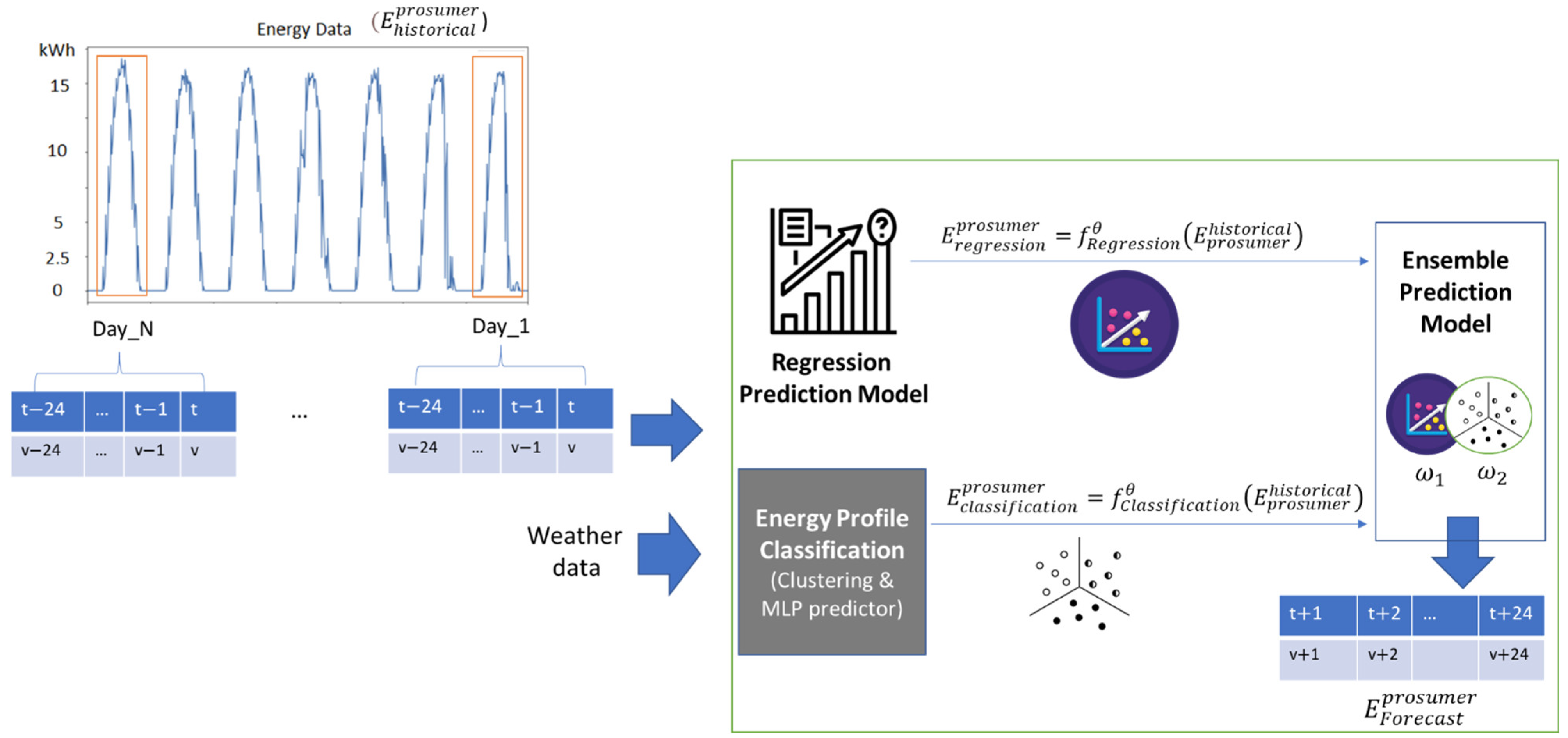
We propose a multi-step energy prediction model (see Figure 1) for prosumers that forecasts the energy values for each hour, $t$, of the next day with respect to the current day denoted as “day” (i.e., 24 steps ahead):

$$E_{predicted}^{prosumer,day}=\left\{e_t^{day+1}\right| t=\left\{1,\dots ,24\right\} and day\in {\mathbb{Z}}^{+} \}.$$

(1)

The features for the energy-prediction model are defined based on energy time-series intervals of 24 h corresponding to days in the past with time intervals of 1 h granularity spreading over the entire monitored data history:

$$E_{historical}^{prosumer,day}=\left\{e_t^{day-d}\right| t=\left\{1,\dots ,24\right\}, d\in \left\{1,2,\dots \right\}\}.$$

(2)

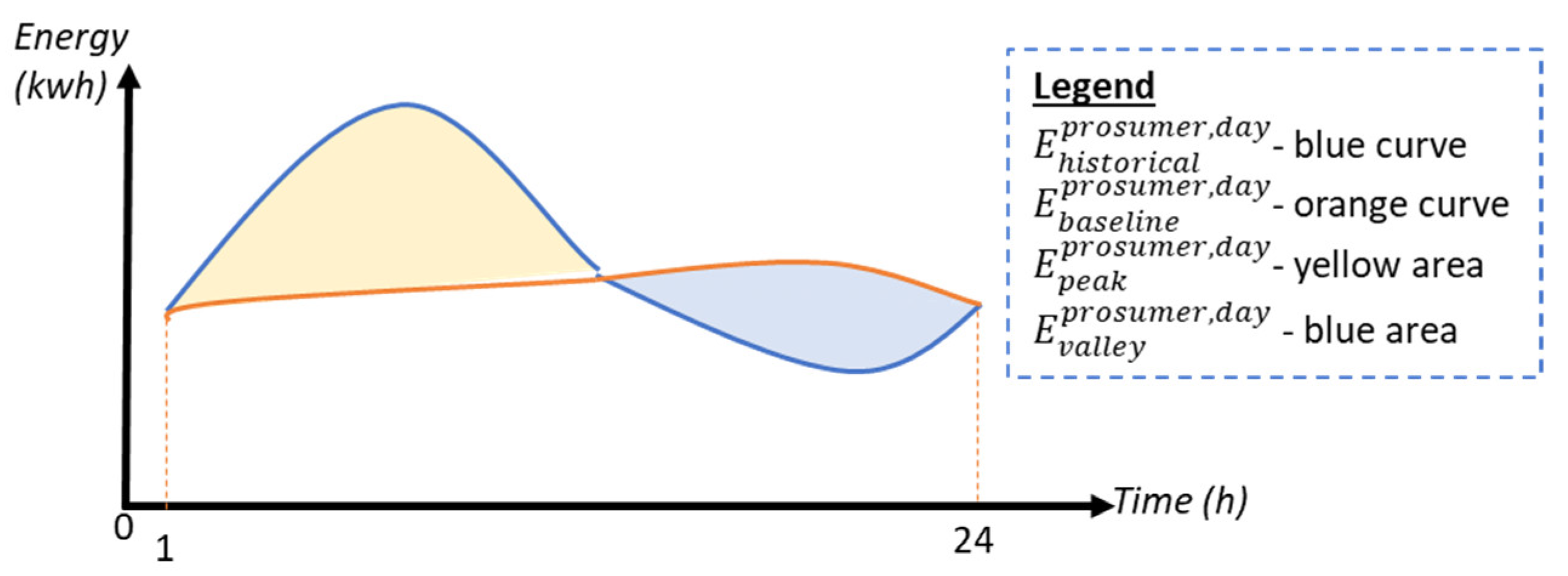
We have considered and extracted relevant energy features by decomposing the energy profiles of the prosumer into three components: energy baseline, valleys, and peaks. This process is shown in Figure 2, where the energy profile is represented with blue, while the baseline profile is colored in orange.

To determine the daily baseline energy profile of a prosumer, we selected and averaged similar intervals from X previous days, with each featuring 24 values for the hours, not including the highest and lowest profiles [2]:

$$E_{baseline}^{prosumer,day}=\frac{1}{X_{days}-2}{{\displaystyle \sum }}_{day \in MID\left(X_{days}\right)}^{X_{days}-2}{E}_{historical}^{prosumer,day}.$$

(3)

where $X_{days}$ represents the number of days in the past considered.

The valleys and the peaks were computed as the energy profile values that are lower or higher than the baseline, as shown in Algorithm 1.

Algorithm 1: Determine Peaks and Valleys

Inputs:$E_{historical}^{prosumer}\left(t\right)$ —historical energy data of prosumer, $t\in \left\{1,\dots ,24\right\}$

$X_{days}—\mathrm{number\; of\; days\; in\; the\; past\; used\; to\; determine\; the\; baseline};$

$day—\mathrm{the\; current\; day\; with\; monitored\; energy\; data}$

$\mathbf{Outputs:} E_{valley}^{prosumer,day}\left(t\right), E_{peak}^{prosumer,day}—\mathrm{the\; energy\; peaks\; and\; valleys\; for\; the\; current} day$

$\mathbf{Begin}$

$E_{historical}^{prosumer,day}=E_{historical}^{prosumer}+E_{current}^{prosumer,day}$ $E_{baseline}^{prosumer,day}=determineBaseline \left(E_{historical}^{prosumer}, X_{days}\right)$ $\mathrm{For\; each\; hour\; t\; of\; the\; day\; do}$ $\mathrm{If} E_{historical}^{prosumer,day}\left(t\right)<E_{baseline}^{prosumer,day}\left(t\right) \mathrm{then}$ $E_{valley}^{prosumer,day}\left(t\right)=E_{historical}^{prosumer,day}\left(t\right)$ $\mathrm{If} E_{historical}^{prosumer,day}\left(t\right)>E_{baseline}^{prosumer,day}\left(t\right) \mathrm{then}$

End

The energy-based features are enhanced by adding contextual information, as we expect different energy profile patterns in different time intervals of a day or for different days in the week or month, etc. The timestamp-derived features allow for the identification of complex and hidden energy patterns and the representation of the time differences in the energy profiles. Weather-related features such as solar irradiance, temperature, or humidity are considered similarly in the prediction process.

The defined energy-prediction model described in Figure 1 uses the above-presented features, and it is based on an ensemble learner to aggregate partial prediction results from regressors and classifiers. A weighted average of two partial predictions is used to handle data heterogeneity, where the sum of the model weights is equal to one:

$$E_{ensemble}^{prosumer}\left(t\right)={\omega }_1\left(t\right)\times E_{classification}^{prosumer}\left(t\right)+(1-{\omega }_1\left(t\right))\times E_{regression}^{prosumer}\left(t\right), \forall t\in \left\{1\dots 24\right\}$$

(4)

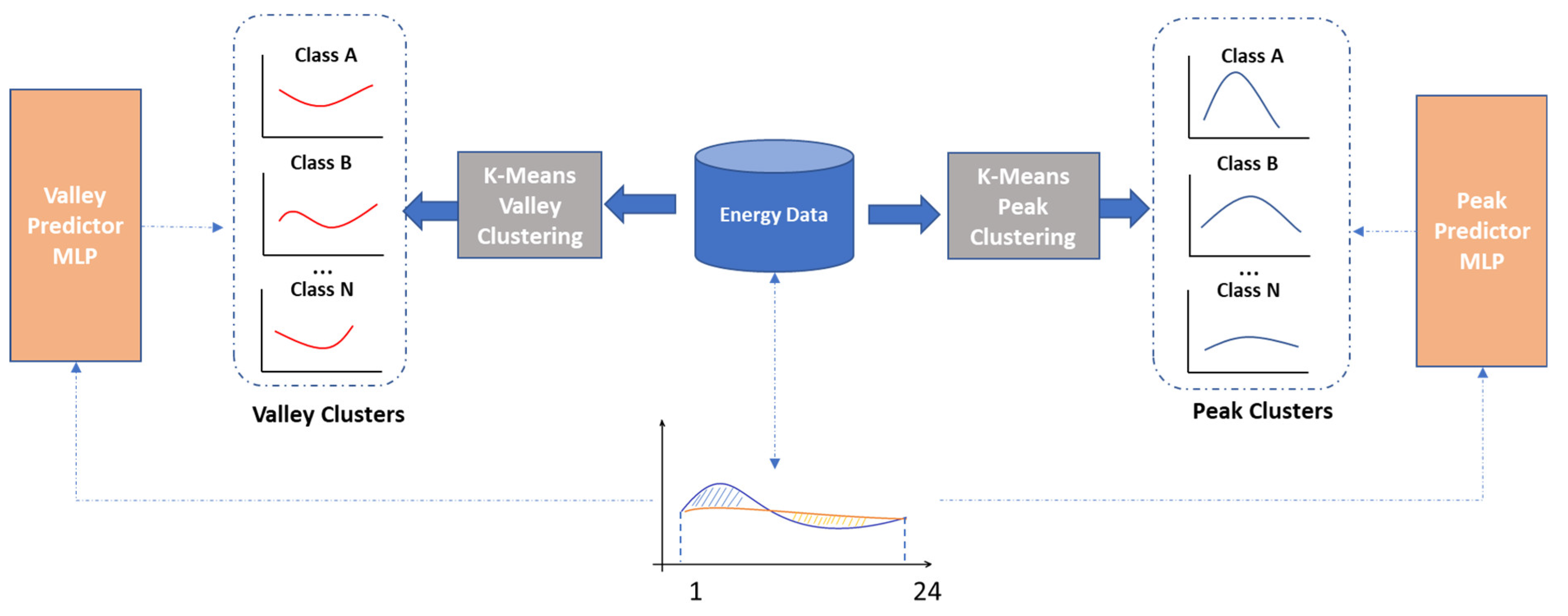
The classification-based models predict the energy peak and valley classes, for the day ahead energy profile of a prosumer using a clustering algorithm (see Figure 3):

$$f_{classify}^{valley}:R^{24}\to \left\{1\dots N_{valley}\right\}, f_{classify}^{valley}\left(E_{valley}^{prosumer,day}\right)=clas{s}_{valley}^k,$$

(5)

$$f_{classify}^{peak}:R^{24}\to \left\{1\dots N_{peak}\right\}, f_{classify}^{peak}\left(E_{peak}^{prosumer,day}\right)=clas{s}_{peak}^k.$$

(6)

The functions $f_{classify}^{valley}$ and $f_{classify}^{peak}$ use K-Means clustering to group the energy valley and energy peak patterns from the historical data of the energy prosumer in $N_{valley}$ and $N_{peak}$ clusters, respectively. We chose K-Means because previous studies in the literature have shown that it is effective in clustering individual households based on their daily energy patterns [49]. However, to our knowledge, it was never applied for classifying the peaks and valleys which may be found inside of a daily energy pattern.

All valley and peak cluster classes, $k$, have as the centroid an energy pattern that is computed as follows ($N_k$ is the number of clusters determined by K-Means, and $t\in \left\{1,\dots ,24\right\}$ hours of the day):

$$mea{n}_{valley}^k\left(t\right)=\frac{1}{N_k}{{\displaystyle \sum }}_{i=1, }^{N_k}{E}_{valley}^{prosume{r}_i}\left(t\right), where E_{valley}^{prosume{r}_i} \in clas{s}_{valley}^k,$$

(7)

$$mea{n}_{peak}^k\left(t\right)=\frac{1}{N_k}{{\displaystyle \sum }}_{i=1}^{N_k}{E}_{peak}^{prosume{r}_i}\left(t\right), where E_{peak}^{prosume{r}_i} \in clas{s}_{peak}^k.$$

(8)

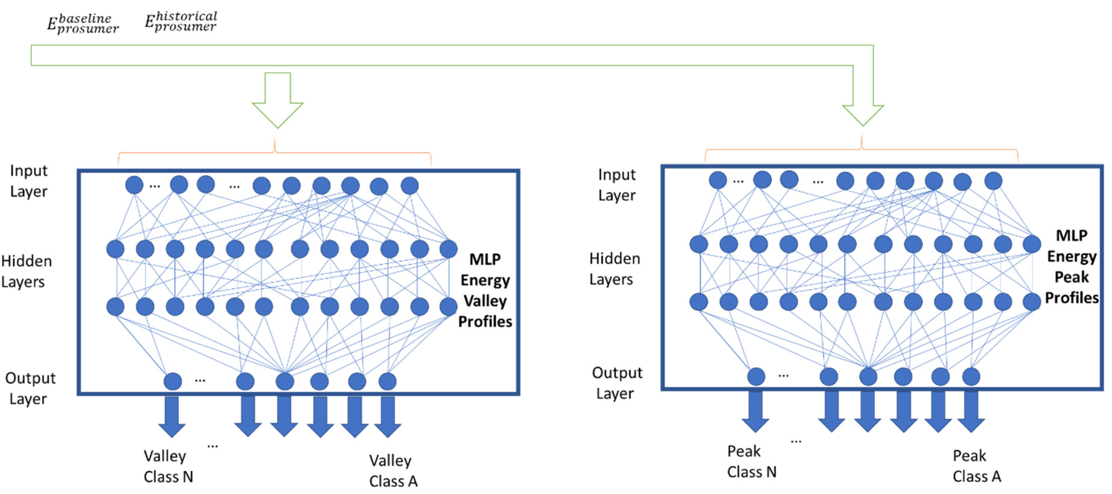
The energy prediction model defines a set of two neural-network-based classifiers that aim to predict the class of the peak and the class of the valley for the next day-ahead prediction. The general architecture of the component is shown in Figure 4. The two neural networks have the same inputs, arrays of length $2\times T+\left|C_F\right|$, where T is the historical data length given as input, and $\left|C_F\right|$ is the cardinality of the contextual feature ($C_F$) set. The inputs of the model are the historical energy data, $E_{prosumer}^{historical}$, over a time interval $\left[0\dots T\right]$ in the past and the baseline of the prosumer, denoted as $E_{baseline}^{prosumer}$.

Furthermore, the models receive as the contextual features derived from the timestamp of the prediction. The predictors can be expressed as functions $f_{peak}$ and $f_{valley}$ which are learned and modeled by using MLP-based neural networks and defined in Equations (9) and (10):

$$f_{peak}:R^{2\times T+\left|C_F\right|}\to \left\{1\dots N_{peak}\right\}, f_{peak}\left(E_{historical}^{prosumer,day}, E_{baseline}^{prosumer,day},C_F\right)=clas{s}_{peak}^{prosumer},$$

(9)

$$f_{valley}:R^{2\times T+\left|C_F\right|}\to \left\{1\dots N_{valley}\right\},f_{valley}\left(E_{historical}^{prosumer,day}, E_{baseline}^{prosumer,day},C_F\right)=clas{s}_{valley}^{prosumer}.$$

(10)

There are several advantages of MLP that have led us to adopt it for this implementation, such as fast development and training, robustness to outliers and missing data, and the fact that it is a universal approximator [50]. At the same time, the MLP network will be eventually translated to a set of non-linear mathematical functions, which, in the case of regression, map the set of input features to set of real numbers. Being feedforward networks, they do not keep track of time, so each classification operation is independent from the last one.

The two predictors, together with the baseline computation component, are put together, as shown in Figure 4, to compute the energy prediction for the prosumer. The components get the historical data from the database and compute the contextual features out of the timestamp. Based on this data, the classifiers defined compute the foreseen peak and valley class for the prosumer.

Knowing the predicted class of the energy valley, $clas{s}_{valley}^{prosumer}$, and the predicted class of the energy peak, $clas{s}_{peak}^{prosumer}$, the energy prediction values for the peak and the valley are determined as being the centroid of the corresponding class.

Finally, the energy prediction is estimated as being the sum of the baseline energy, the centroid of the peak class, and the centroid of the valley class, as shown in Equation (11):

$$E_{classification}^{prosumer}=E_{baseline}^{prosumer}-E_{valley}^{prediction}+E_{peak}^{prediction}.$$

(11)

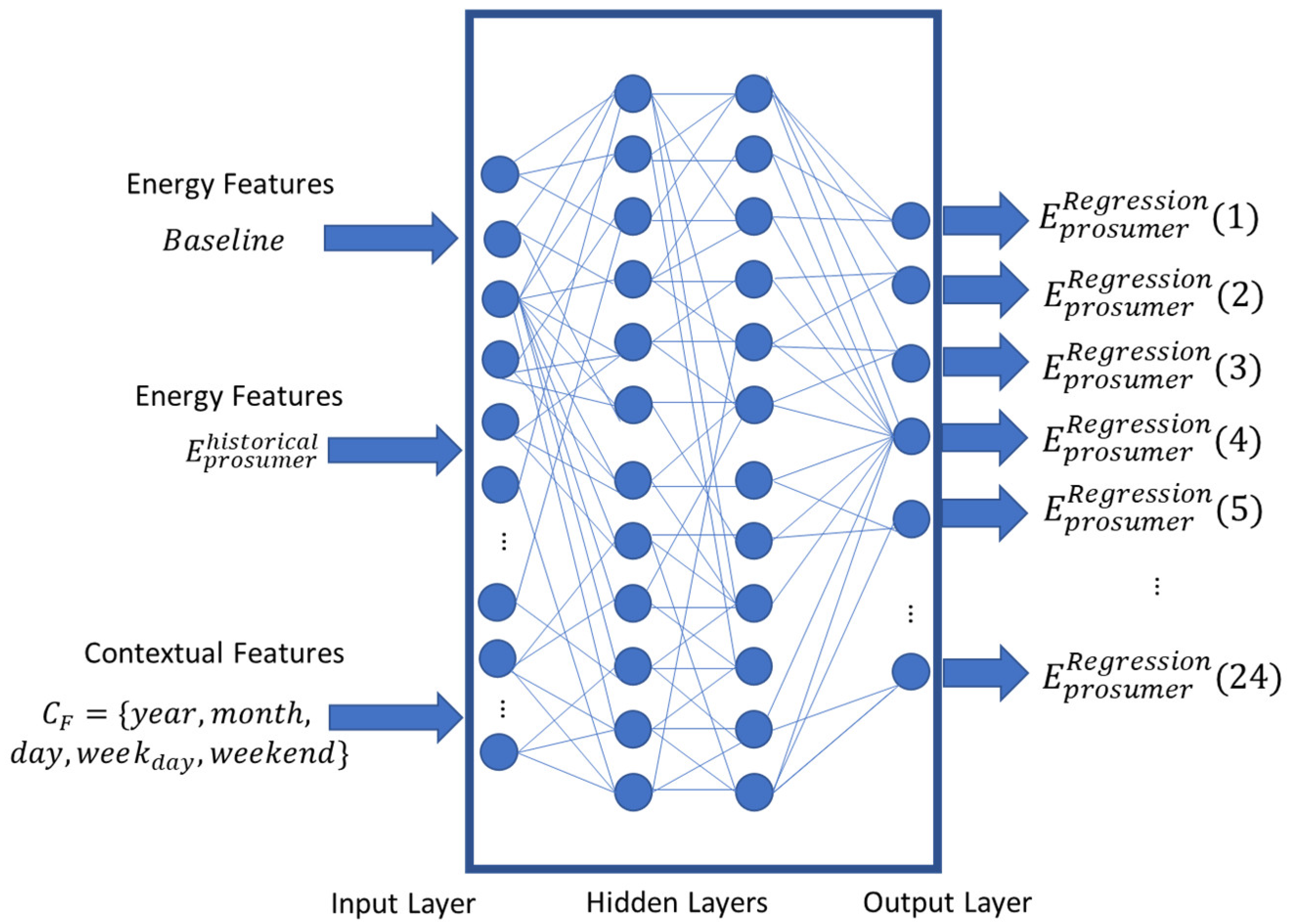
In case of the energy prediction model based on regression, we are aiming to estimate the finer granularity fluctuations of the energy-consumption patterns. Thus, we define a regressor having the same inputs as the classifier above, but, as outputs, it should have the energy patterns for the prediction window:

$$f_{regression}:R^{2\times T+\left|C_F\right|}\to R^T, f_{regression}\left(E_{historical}^{prosumer}, E_{baseline}^{prosumer},C_F\right)=E_{regression}^{prosumer}.$$

(12)

The function $f_{regression}$ is learned by using a multilayer perceptron (MLP), depicted in Figure 5, having as inputs the $E_{historical}^{prosumer}$ over an interval in the past; the baseline $E_{baseline}^{prosumer}$; and a set of contextual features, such as year, month, day, day of week, season, and holiday. The output of the model is a set of T values, $E_{regression}^{prosumer}$, where the value from index h represents the energy consumption prediction for hour, $h$.

4. Evaluation Results

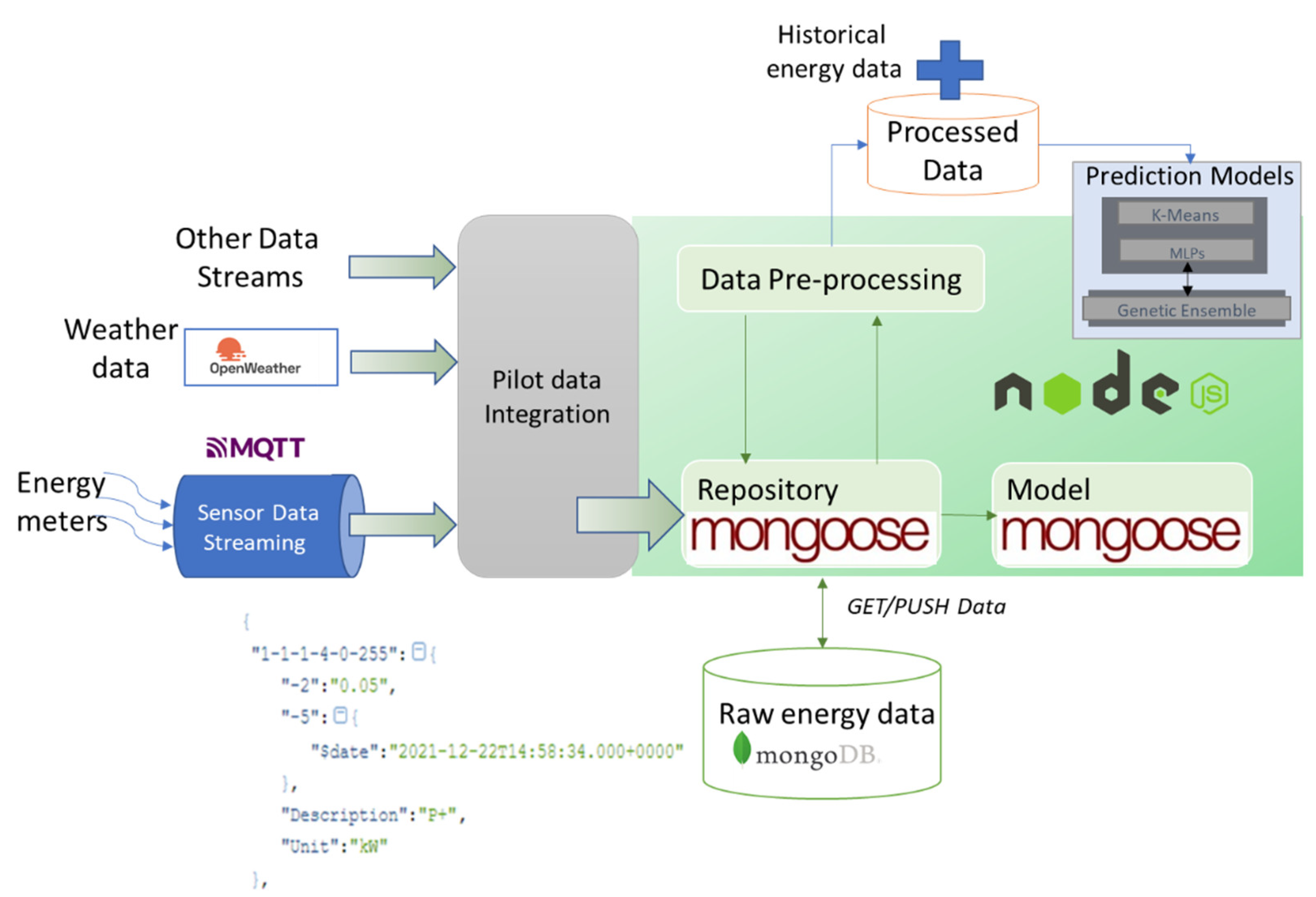
The proposed energy-prediction solution was implemented in a proof-of-concept prototype that has three main components (see Figure 6): (i) the prosumer data integration (i.e., hardware monitoring infrastructure with the data storage), (ii) the preprocessing of raw data, and (iii) the deep-learning models for energy prediction.

From smart energy meters, the data are sent through MQTT queues. It contains the monitored value, the timestamp, the measuring unit, and the sensor ID. An MQTT listener checks for new samples, and all data received are validated and inserted into a MongoDB NoSQL database. The interaction with MongoDB is made with the Mongoose framework that facilitates the data-validation process before inserting it into the database. The weather data (e.g., temperature, humidity, etc.) is collected and used as a feature to improve the energy-demand prediction. We are using periodical requests to weather APIs with the areas in which the smart meters are installed.

A data-preprocessing thread is associated with each sensor and scheduled to run every hour. The data are converted if necessary and aggregated over one hour, and the missing data are handled by using a multiplicative seasonal method for imputation. The processed database stores the field device configuration, the energy data, and the prediction results. It can store the hourly energy values, the determined clusters, and data needed for model training, such as the daily baseline demand, the valleys, and the peaks. The historical datasets used for evaluation are directly fed into this database. The prediction module implements the prediction algorithms. The K-Means model used for clustering is developed by using the Weka library and the configurable MLP models by using the Deep java library. The input for the MLP is defined as a generic map to enable the model’s training with a different number of features.

We used historical and live energy data streams acquired from the smart meters associated with energy prosumers [51] to evaluate the energy-prediction solution. Combinations of energy and weather features for two categories of prosumers have been considered to determine the energy-prediction accuracy (see

Table 1. Energy-prediction evaluation test cases.

Type	Characteristics	Evaluation Setup				Evaluation Case ID
		Prediction Features			Live Energy Data Streams
		Energy	Temperature	Humidity
Small	- Maximum energy demand: 13.7 kWh - Four years of monitored data - 15 min the Granularity of the monitored data	Yes	No	No	No	TC-S1
		Yes	No	No	Yes	TC-S2
		Yes	Yes	No	Yes	TC-S3
Medium	- Maximum energy demand: 260 kWh - Three years of monitored data: - 1 h the granularity of the monitored data	Yes	No	No	No	TC-M1
		Yes	Yes	No	No	TC-M2
		Yes	No	Yes	No	TC-M3

). The models are re-trained on a daily basis, and a thread is scheduled to make predictions in day-ahead (i.e., 24 energy values, one for each hour of the next day).

4.1. Small-Scale Prosumer

For the first evaluation case (TC-S1), historical data from a prosumer with a low energy demand was used to train the models and evaluate the energy prediction results. The data were split in 60% for models training, 20% for validation and weight computation, and 20% for prediction testing.

The clustering was made on the 24-energy consumption peaks’ and valleys’ values computed daily concerning the baseline energy profile. Figure 7 shows the centers of the clusters determined. In the case of the peak profiles, there are two clusters representing periods with very low energy consumption (0–0.5 kWh), two clusters representing periods with increased energy consumption in the intervals (6–11 and 9–14), and one cluster for profiles where the energy consumption is increased for hour interval 6–19. In the case of the valleys, four clusters store profiles representing a small constant decrease in energy consumption and five cluster aggregate profiles indicating a significant decrease in consumption at different time intervals during the day.

Over 1000 epochs were used to train the prediction models. The weights for the models were found by using the genetic algorithm and saved in the database to compute the final predicted values by ensemble the individual prediction results. The average SMAPE (Symmetric Mean Absolute Percentage Error) was approx. 6.5%, and the minimum error obtained for one day was 2.44%. The best predicted day can be seen in Figure 8. SMAPE was selected because it measures accuracy based on a percentage that is scale-independent and, therefore, can be used for comparing the energy prediction of prosumers with different energy scales [49,52]. Moreover, it is symmetric having both lower and upper bounds addressing one of the main disadvantages of MAPE.

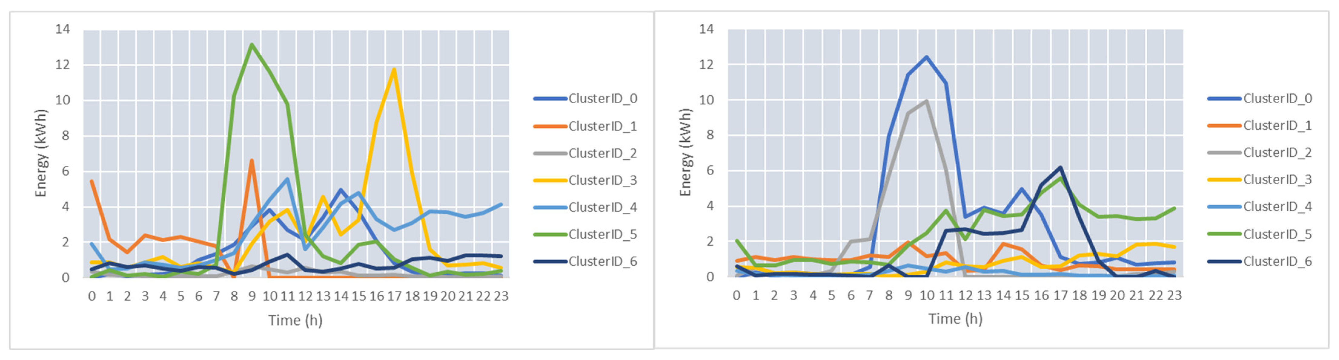
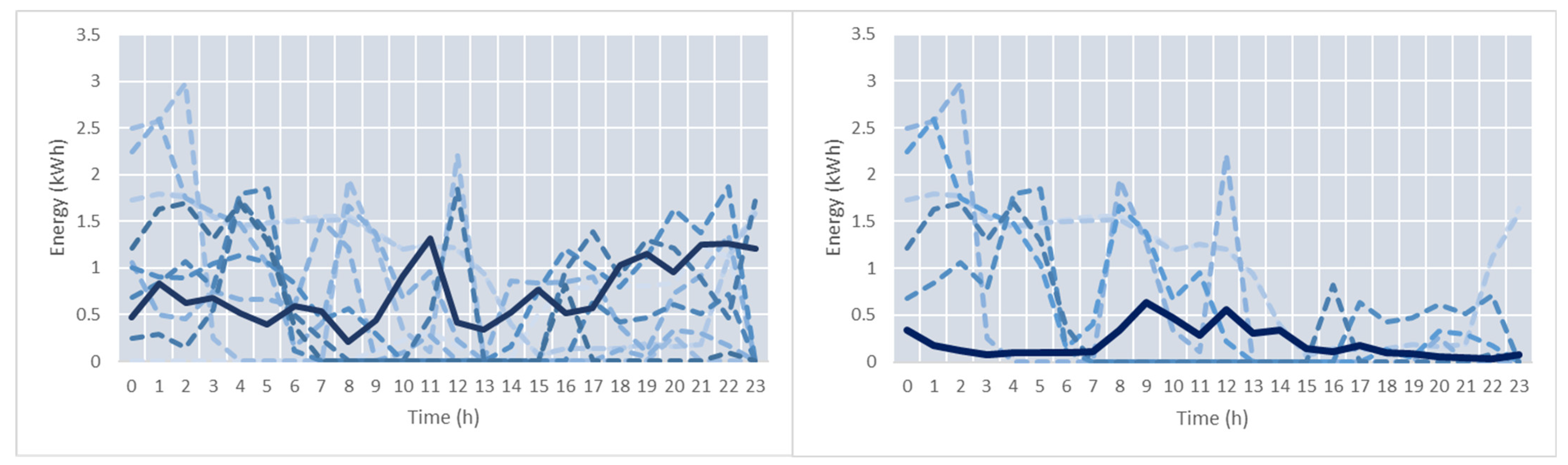
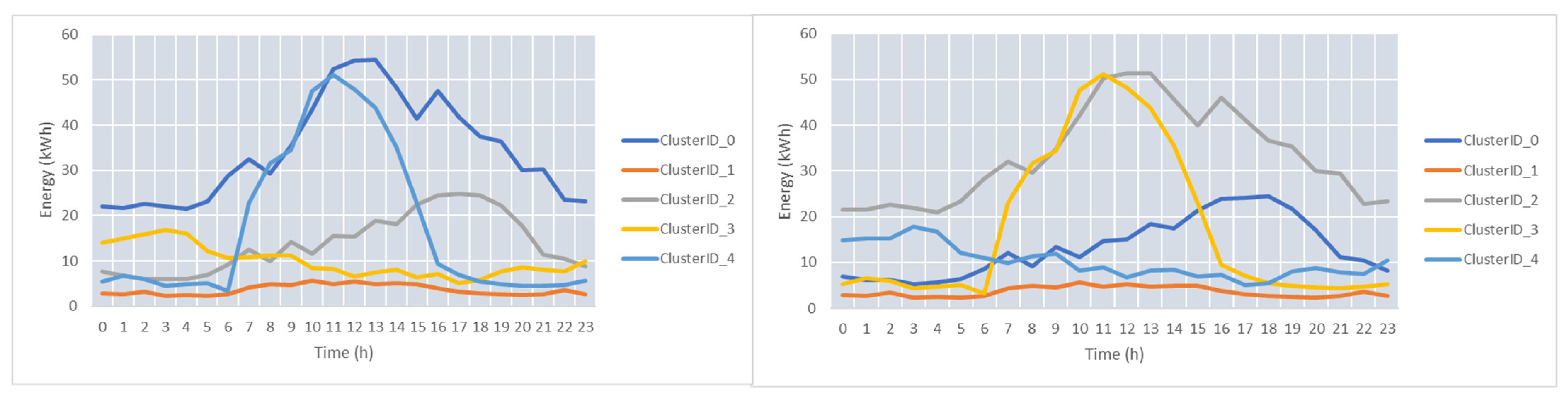
In the case of test cases, TC-S2 and TC-S3 energy data streams are collected in real-time for three months and used for model training and energy prediction. We use the same energy prediction methodology. The daily baseline is computed to determine the energy peak and valley values. The K-Means algorithm is applied to daily energy patterns to cluster the peaks’ and valleys’ profiles.

The distance from each energy profile to the cluster centroids is computed by using a 24-dimensional Euclidean distance. Figure 9 shows the centers of the clusters. Seven clusters for the peaks and seven for the valleys were determined. Figure 10 presents the energy profiles for the peaks and valleys of the clusters with the ID_6 and ID_3, respectively.

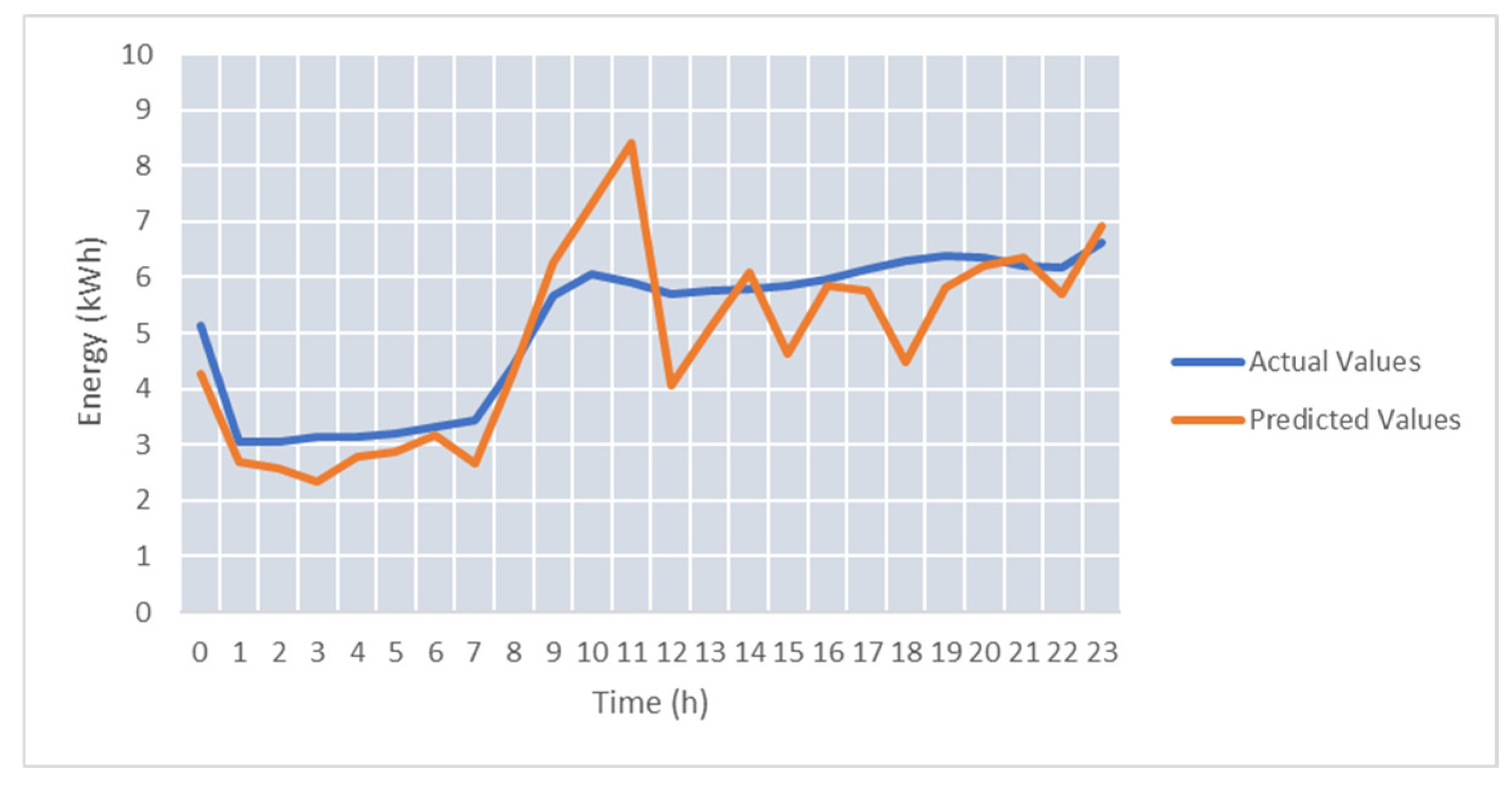
For test case TC-S2, we used only energy features. The higher variability of live energy data streams and the size of the training data affect the accuracy of the energy prediction. The average SMAPE was 37.58%. Figure 11 shows the energy predicted values, considering the monitored energy data stream for 24 h.

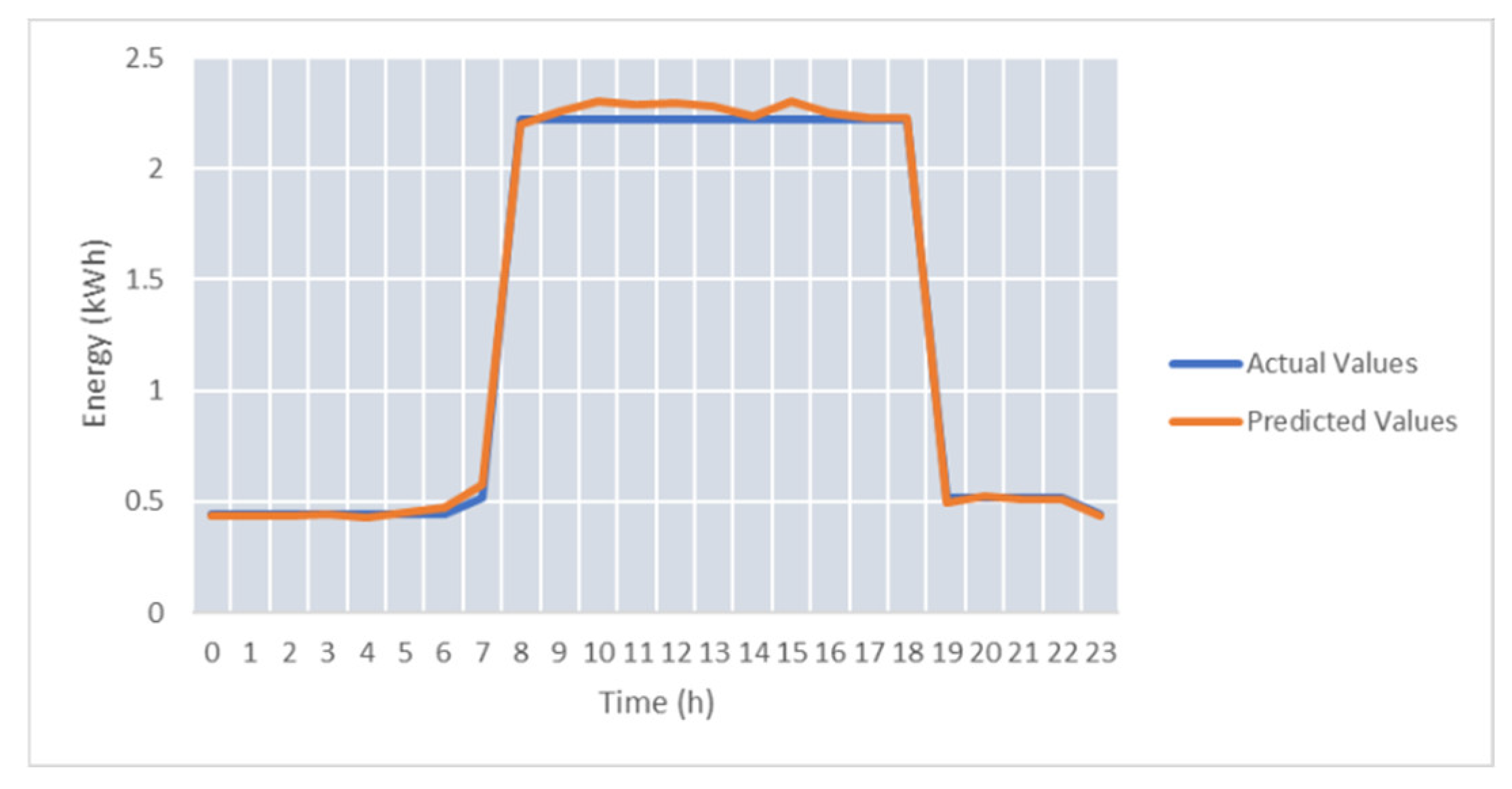
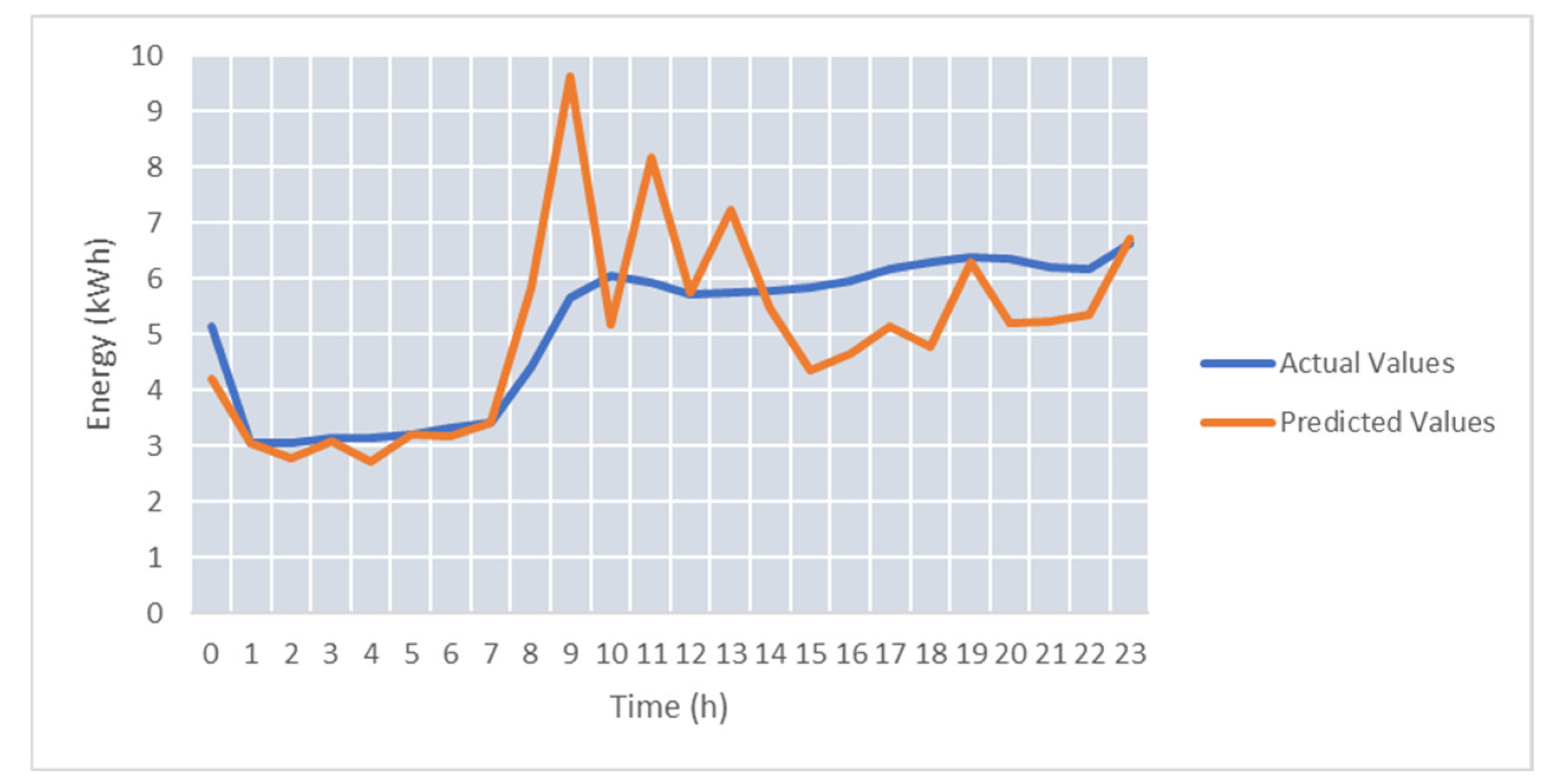
To improve the accuracy of the energy prediction on real-time data streams in test case TC-S3, we considered temperature as an additional feature. After we added the temperature sensor to the model training, the average SMAPE was 29.9%. Figure 12 shows the prediction improvement compared to Figure 11. The forecasted energy values follow with better accuracy the actual energy profile.

As it can be seen, the use of temperature as a feature brings a significant improvement for the energy prediction values, with the SMAPE decreasing for the best predicted day from 14.9 down to 9.06.

4.2. Medium Scale Prosumer

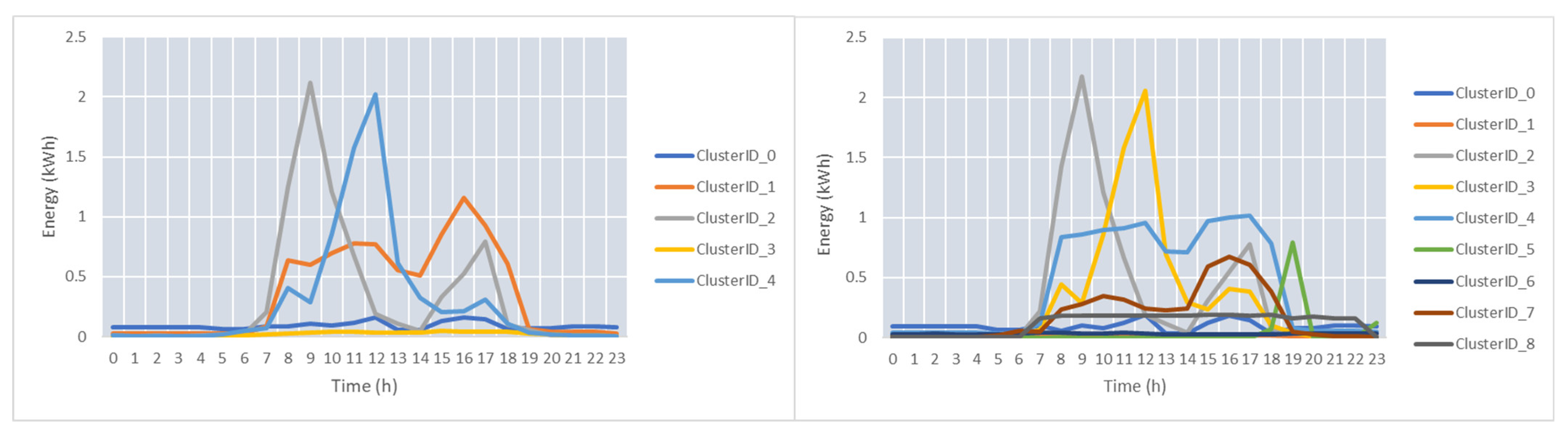
For medium-scale prosumer, five clusters representing the peak profiles and five clusters representing the valleys profiles were identified. The centroids of the clusters can be seen in Figure 13.

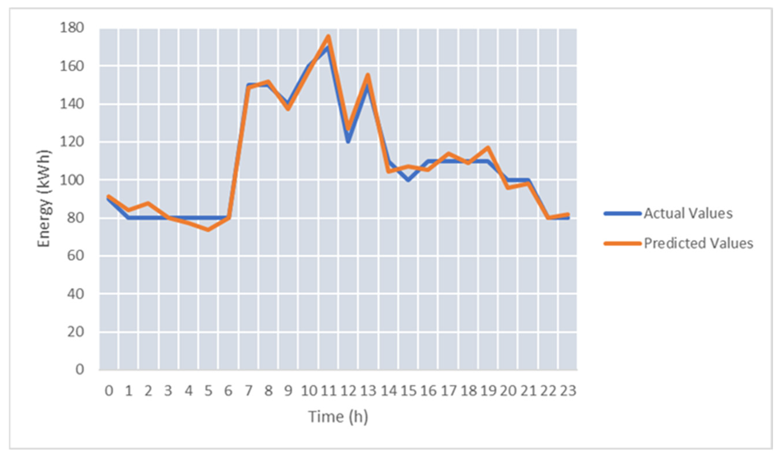
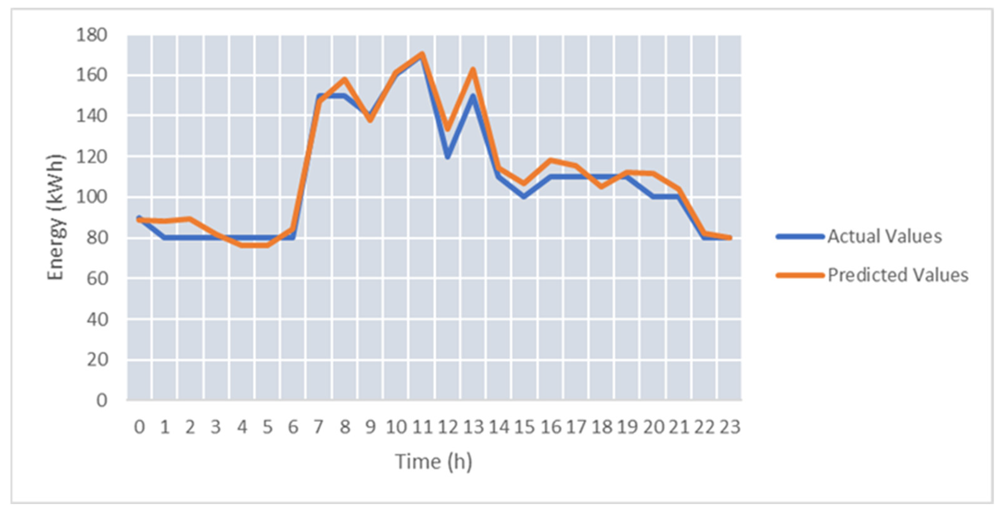
For the first test case, TC-M1, we have considered only the energy features in the prediction configuration. The training configuration of the models (i.e., splits size of data—60%, 20%, and 20%; number of epochs—over 1000) was similar to the previous evaluation cases. The average SMAPE was about 14%, while the minimum value was 4.8% (see Figure 14).

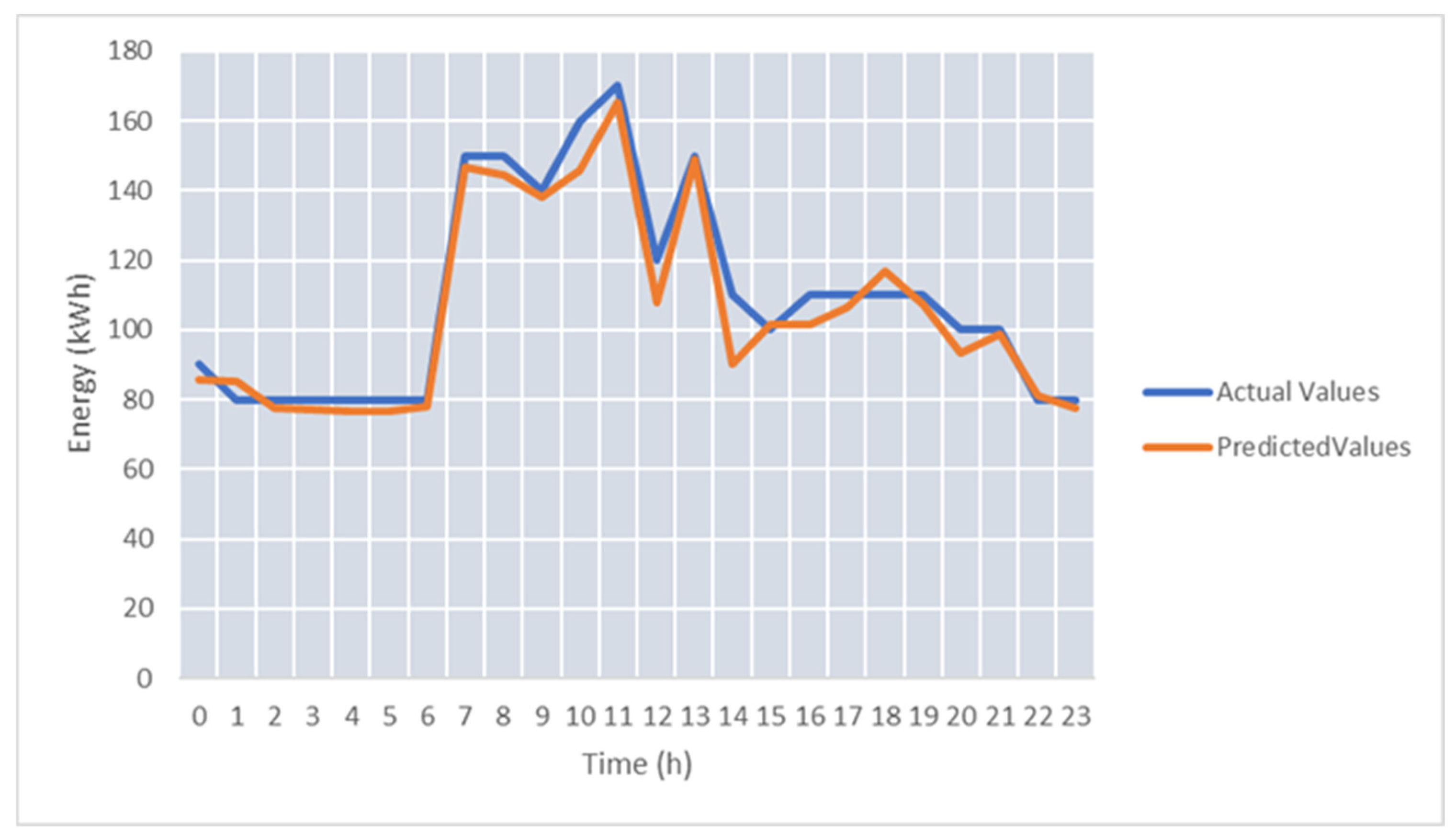
We have considered the temperature taken from weather services as a feature to improve the prediction accuracy (i.e., test case TC-M2). With a higher number of epochs, the accuracy was improved, with the average SMAPE being around 12%, and the SMAPE for the best predicted was 4.7% (see Figure 15).

In the last tested configuration, TC-M3, the temperature sensor was substituted with a humidity sensor, and slightly better results were obtained, with a lower best SMAPE (see Figure 16).

5. Conclusions and Discussion

In this paper, we have proposed a deep neural network model for day-ahead prediction of energy profiles of prosumers. Such energy prediction is a prerequisite for their active participation in energy grid management. Our model uses an ensemble of classification-based models used to cluster similar energy profiles and regression models used to fine-tune the energy prediction. We propose and successfully used the peaks and valleys of the energy profile with respect to the energy baseline as features of the learning process. Our solution addresses some of the challenges related to the use of machine learning models for energy prediction. As most of the literature is focused on one-step-ahead energy prediction, we provide a solution for the significantly difficult case of multi-step energy prediction in which 24 values are predicted in advance, corresponding to a day-ahead prediction at one hour granularity. We are not using only the raw monitored energy, but we also collect several energy-based features that are correlated with weather information. Moreover, the prediction model was tested not only on historical datasets, but also on prosumers feeding real-time energy data. We have provided a prosumer integrated solution, and the real-time data streams of energy data were considered in the training and prediction process. The software infrastructure defined allows the integration of real-time energy data streams with the deep learning models’ training and prediction.

Table 2. Energy prediction results.

Evaluation Case ID	SMAPE
	Best	Average
TC-S1	2.44%	6.5%
TC-S2	14.9%	37.58%
TC-S3	11.2%	29.9%
TC-M1	4.8%	14%
TC-M2	4.7%	12%
TC-M3	3.38%	12%

summarizes the energy prediction results for the various test case configurations used. For the small-scale prosumer, when the historical data are available, the results are significantly better than the real-time predictions, where less and more scarce energy data are available. The additional weather information, such as temperature, improves the accuracy but has a small impact on the prediction results. In the case of the medium-scale prosumer, when additional weather sensors (e.g., temperature and humidity) were added, the predictions improved significantly, and the average SMAPE decreased from 14% to 12%.

For the small-scale prosumer, the lowest average SMAPE (6.5%) is in the case in which historical data are available for a longer period (TC-S1). The performance achieved by the models in this evaluation case is higher than for the medium energy prosumer with a training set similar in size, where the average SMAPE is between 12% and 14%. The number of identified peaks’ and valleys’ clusters corresponding to energy consumption patterns is not higher than in the case of the small prosumer. Thus, the errors for the second prosumer can be due to a higher range of variation for the energy consumption values in the same cluster. A higher number of clusters can bring improvements for the best predicted days, but the general performance would be affected by the higher complexity of peaks and valleys classes prediction due to more similarities between clusters. Moreover, the first prosumer has a lower best-predicted day error than the prosumer with higher energy consumption (2.44% for the small prosumer, and 4.8% for the medium prosumer) when only the energy historical features are used for prediction.

In the evaluation cases using live energy data streams, the data available for training are on a shorter period, and the performance of the predictions is affected. For the small prosumer (TC-S2), if only the historical energy consumption is used, the average SMAPE is 37.58%. When the monitored temperature is added in the features set (TC-S2), the average SMAPE is significantly lower (29.9%), and there are also improvements for the best cases from 14.9% to 11.2%. When more features that correlate energy consumption are available, such as the temperature, the prediction accuracy is higher. The improvements brought by additional weather data can also be observed in the case of the medium-scale prosumer when temperature and humidity data were considered in two test scenarios (TC-M2 and TC-M3). The best prediction day has a lower error for both test scenarios, but a significant improvement is shown for the worst predicted day error that decreases consistently.

As future work, we plan to combine the black-box machine learning models with the white-box models provided as digital twins of energy assets. We will move toward the direction of physical informed machine learning by developing a hybrid solution that integrates physical realities and data model predictions to capture finer-grained details and provide more precise predictions. Digital twins’ models of the energy assets will be used to model the physical features and to conduct data-driven simulations for better understanding their fine-grained energy behavior, operational constraints, and optimal integration/usage with multi-energy services. Moreover, such models will allow the generation of data with better quality that will cover non-optimal situations and will complement the monitored data. For the black-box models, we will implement deep neural network models that can be used on top of the big data-processing infrastructure, while considering the comprehensive modeling of demand and supply provided by the digital twins. Lambda architectures could be used to dispatch heterogenous monitored data to both a batch layer managing historical datasets and a speed layer for managing closer to the real-time streams of data. Finally, the coupling and association of energy data with other non-energy vector data, such as social data or cross-sectors’ data, can be investigated, with a view of generating more accurate predictions.