
Three-Dimensional Acoustic Analysis of a Rectangular Duct with Gradient Cross-Sections in High-Speed Trains: A Theoretical Derivation


Abstract
:Featured Application
Abstract
1. Introduction
2. 3D Analytical Solutions to the Wave Equations of a RDGC
2.1. 3D Solutions for a Straight Rectangular Duct
2.2. 3D Solutions for a RDGC
3. Derivation of the TM for a RDGC
4. The TMs and TLs of Rectangular Expansion Chambers (RECs)
4.1. The TMs of the RECs with One or Double Baffles
4.2. Geometries of the RECs
4.3. Calculation and Measurement of the TLs for the RECs
5. Results
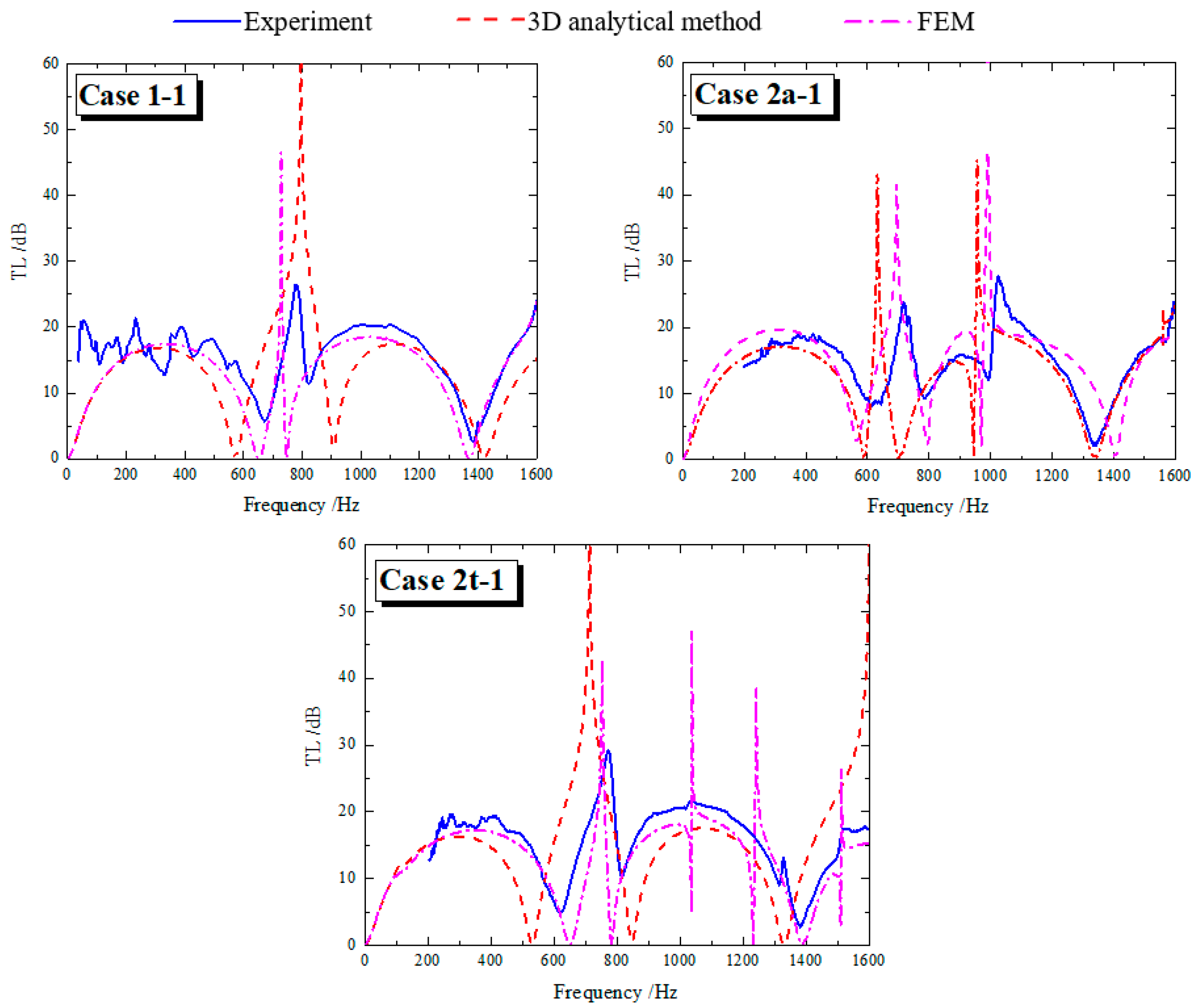
5.1. Experimental Validation of the Calculated Results
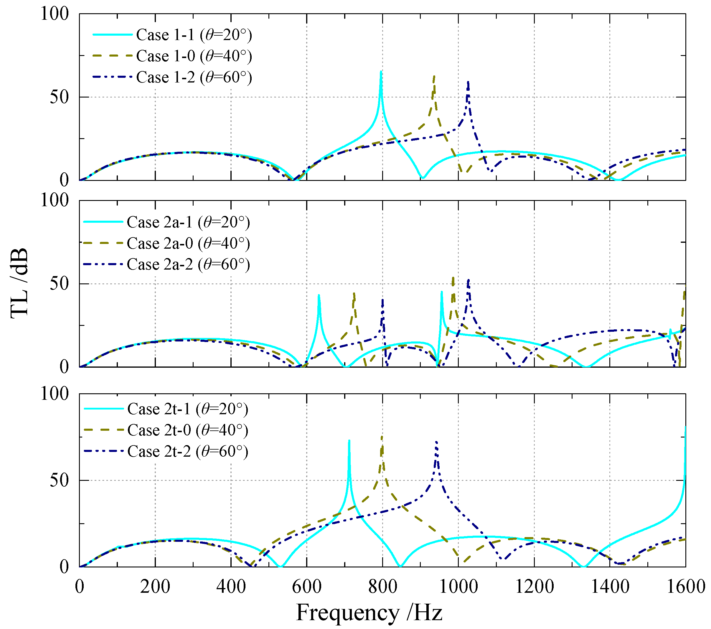
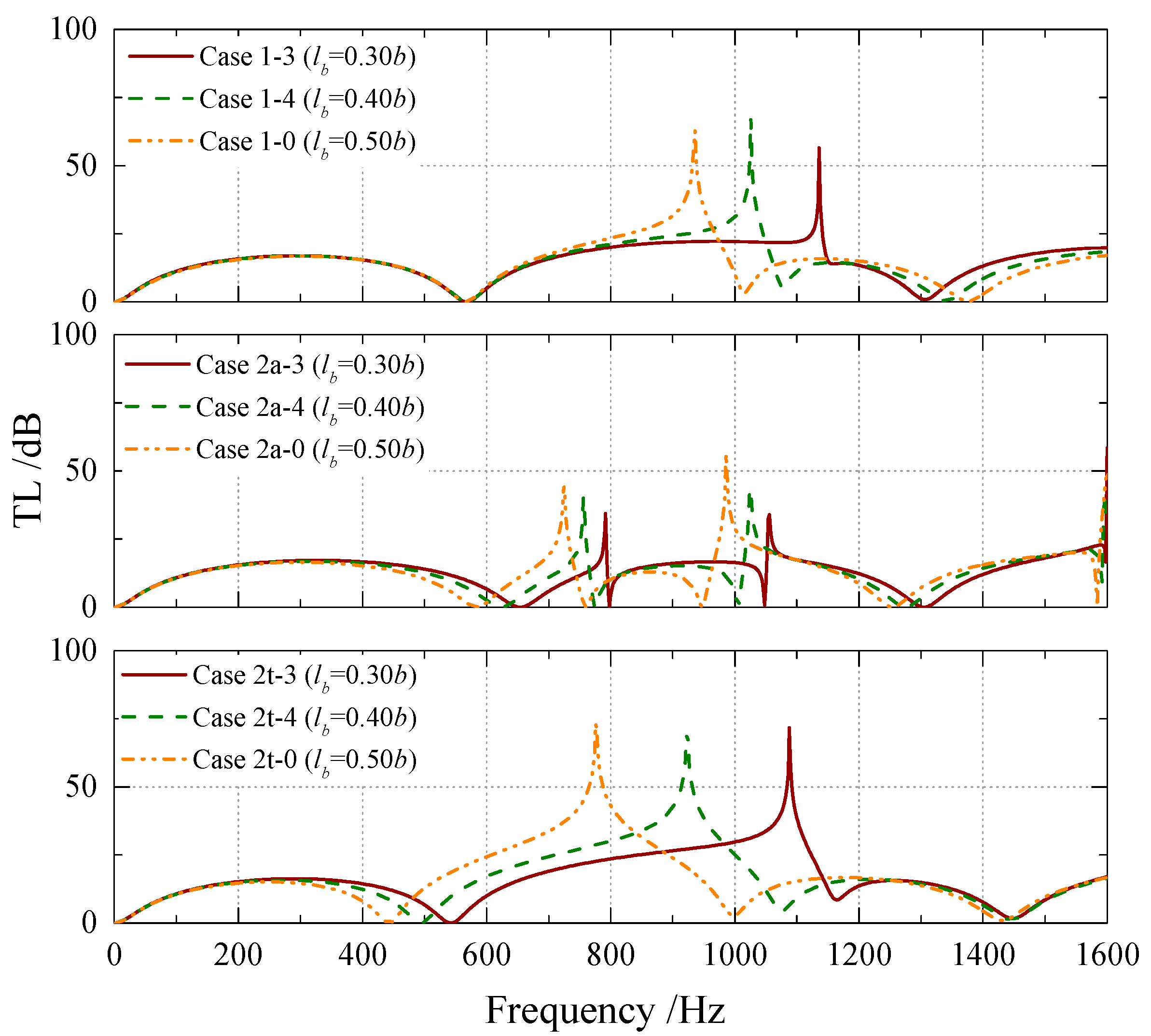
5.2. TLs of the RECs
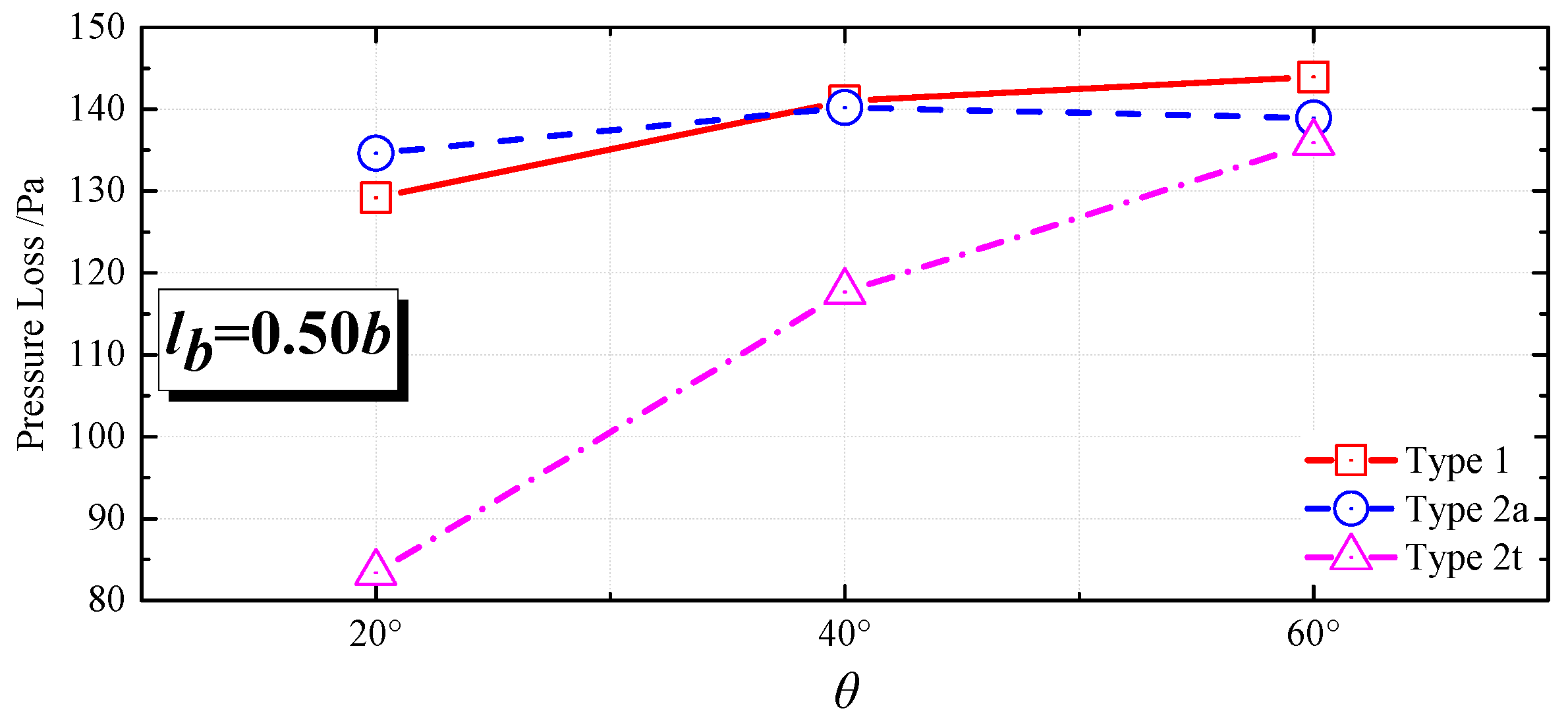
5.3. Pressure Losses of the RECs
6. Conclusions
Author Contributions
Funding
Institutional Review Board Statement
Informed Consent Statement
Data Availability Statement
Conflicts of Interest
Appendix A. Derivation of the A, B, C and D in the TM
Appendix B. FEM Methodology

References
- Sun, Y.H.; Zhang, J.; Han, J.; Gao, Y.; Xiao, X.B. Acoustic transmission characteristics and optimum design of the wind ducts of high-speed train. J. Mech. Eng. Chin. Ed. 2018, 54, 129–137. (In Chinese) [Google Scholar] [CrossRef]
- Sun, Y.H.; Zhang, J.; Han, J.; Gao, Y.; Xiao, X.B. Sound transmission characteristics of silencer in wind ducts of high-speed train. J. Zhejiang Univ. Eng. Sci. 2019, 53, 1389–1397. (In Chinese) [Google Scholar]
- Gopalakrishnan, S.; Raut, M.S. Longitudinal wave propagation in one-dimensional waveguides with sinusoidally varying depth. J. Sound Vib. 2019, 463, 114945. [Google Scholar] [CrossRef]
- Assis, G.F.C.A.; Beli, D.; Miranda, E.J.P., Jr.; Camino, J.F.; Dos Santos, J.M.C.; Arruda, J.R.F. Computing the complex wave and dynamic behavior of one-dimensional phononic systems using a state-space formulation. Int. J. Mech. Sci. 2019, 163, 105088. [Google Scholar] [CrossRef]
- Liu, J.; Wang, T.; Chen, M. Analysis of sound absorption characteristics of acoustic ducts with periodic additional multi-local resonant cavities. Symmetry 2021, 13, 2233. [Google Scholar] [CrossRef]
- Terashima, F.J.H.; de Lima, K.F.; Barbieri, N.; Barbieri, R.; Filho, N.L.M.L. A two-dimensional finite element approach to evaluate the sound transmission loss in perforated silencers. Appl. Acoust. 2022, 192, 108694. [Google Scholar] [CrossRef]
- Junge, M.; Brunner, D.; Walz, N.-P.; Gaul, L. Simulative and experimental investigations on pressure-induced structural vibrations of a rear muffler. J. Acoust. Soc. Am. 2010, 128, 2782–2791. [Google Scholar] [CrossRef]
- Liu, L.L.; Zheng, X.; Hao, Z.Y.; Qiu, Y. A computational fluid dynamics approach for full characterization of muffler without and with exhaust flow. Phys. Fluids 2020, 32, 066101. [Google Scholar]
- Liu, L.L.; Hao, Z.Y.; Zheng, X.; Qiu, Y. A hybrid time-frequency domain method to predict insertion loss of intake system. J. Acoust. Soc. Am. 2020, 148, 2945. [Google Scholar] [CrossRef]
- Liu, L.L.; Zheng, X.; Hao, Z.Y.; Qiu, Y. A time-domain simulation method to predict insertion loss of a dissipative muffler with exhaust flow. Phys. Fluids 2021, 33, 067114. [Google Scholar] [CrossRef]
- Tolstoy, I. The WKB approximation, turning points, and the measurement of phase velocities. J. Acoust. Soc. Am. 1972, 52, 356–363. [Google Scholar] [CrossRef]
- Subrahmanyam, P.B.; Sujith, R.I.; Lieuwen, T.C. A family of exact transient solutions for acoustic wave propagation in inhomogeneous, non-uniform area ducts. J. Sound. Vib. 2001, 240, 705–715. [Google Scholar] [CrossRef]
- Li, J.; Morgans, A.S. The one-dimensional acoustic field in a duct with arbitrary mean axial temperature gradient and mean flow. J. Sound. Vib. 2017, 400, 248–269. [Google Scholar] [CrossRef]
- Rani, V.K.; Rani, S.L. WKB solutions to the quasi 1-D acoustic wave equation in ducts with non-uniform cross-section and inhomogeneous mean flow properties—Acoustic field and combustion instability. J. Sound. Vib. 2018, 436, 183–219. [Google Scholar] [CrossRef]
- Basu, S.; Rani, S.L. Generalized acoustic Helmholtz equation and its boundary conditions in a quasi 1-D duct with arbitrary mean properties and mean flow. J. Sound. Vib. 2021, 512, 116377. [Google Scholar] [CrossRef]
- Eisner, E. Complete solutions of the “Webster” horn equation. J. Acoust. Soc. Am. 1967, 41, 1126–1146. [Google Scholar] [CrossRef]
- Miles, J.H. Verification of a one-dimensional analysis of sound propagation in a variable area duct without flow. J. Acoust. Soc. Am. 1982, 72, 621–624. [Google Scholar] [CrossRef]
- Lee, S.K.; Mace, B.R.; Brennan, M.J. Wave propagation, reflection and transmission in non-uniform one-dimensional waveguides. J. Sound. Vib. 2007, 304, 31–49. [Google Scholar] [CrossRef]
- Martin, P.A. On Webster’s horn equation and some generalizations. J. Acoust. Soc. Am. 2014, 116, 1381–1388. [Google Scholar] [CrossRef] [Green Version]
- Donskoy, D.M. Directionality and gain of small acoustic velocity horns. J. Acoust. Soc. Am. 2017, 142, 3450–3458. [Google Scholar] [CrossRef]
- Pagneux, V.; Amir, N.; Kergomard, J. A study of wave propagation in varying cross-section waveguides by modal decomposition. Part I. Theory and validation. J. Acoust. Soc. Am. 1996, 100, 2034–2048. [Google Scholar] [CrossRef]
- Amir, N.; Pagneux, V.; Kergomard, J. A study of wave propagation in varying cross-section waveguides by modal decomposition. Part II. Results. J. Acoust. Soc. Am. 1997, 101, 2504–2517. [Google Scholar] [CrossRef] [Green Version]
- Maurel, A.; Mercier, J.F.; Pagneux, V. Improved multimodal admittance method in varying cross section waveguides. Proc. Math. Phys. Eng. Sci. 2014, 470, 20130448. [Google Scholar] [CrossRef] [PubMed]
- Pillai, M.A.; Ebenezer, D.D.; Deenadayalan, E. Transfer matrix analysis of a duct with gradually varying arbitrary cross-sectional area. J. Acoust. Soc. Am. 2019, 146, 4435–4445. [Google Scholar] [CrossRef] [PubMed]
- Munjal, M.L. Acoustics of Ducts and Mufflers, 2nd ed.; John Wiley & Sons: New York, NY, USA, 2014. [Google Scholar]
- Polyanin, A.D.; Zaitsev, V.F. Handbook of Exact Solutions for Ordinary Differential Equations; CRC Press: Boca Raton, FL, USA, 1995. [Google Scholar]
- Fucci, G.; Kirsten, K. Expansion of infinite series containing modified Bessel functions of the second kind. J. Phys. A Math. Theor. 2015, 48, 435203. [Google Scholar] [CrossRef] [Green Version]
- Torregrosa, A.J.; Broatch, A.; Payri, R. A study of the influence of mean flow on the acoustic performance of Herschel–Quincke tubes. J. Acoust. Soc. Am. 2000, 107, 1874–1879. [Google Scholar] [CrossRef]
- Ih, J.G. The reactive attenuation of rectangular plenum chambers. J. Sound. Vib. 1992, 157, 93–122. [Google Scholar] [CrossRef]
- Mechel, F.P. Formulas of Acoustics, 2nd ed.; Springer: Berlin/Heidelberg, Germany, 2008. [Google Scholar]
- ASTM E2611-09; Standard Test Method for Measurement of Normal Incidence Sound Transmission of Acoustical Materials Based on the Transfer Matrix Method. ASTM International: West Conshohocken, PA, USA, 2009.
- ANSYS Inc. Ansys Fluent 19.1 Theory Guide; ANSYS Inc.: Canonsburg, PA, USA, 2018. [Google Scholar]
- Fu, J.; Chen, W.; Tang, Y.; Yuan, W.H.; Li, G.M.; Li, Y. Modification of exhaust muffler of a diesel engine based on finite element method acoustic analysis. Adv. Mech. Eng. 2015, 7, 1–2. [Google Scholar] [CrossRef]


| Unit | TM | Annotations |
|---|---|---|
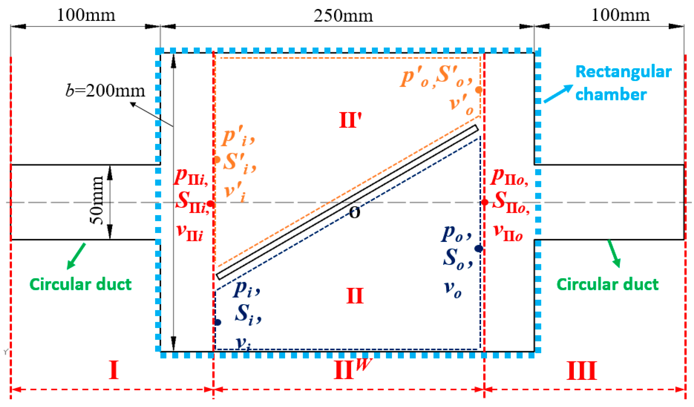
| I | —made of two uniform ducts and one sudden expansion section | |
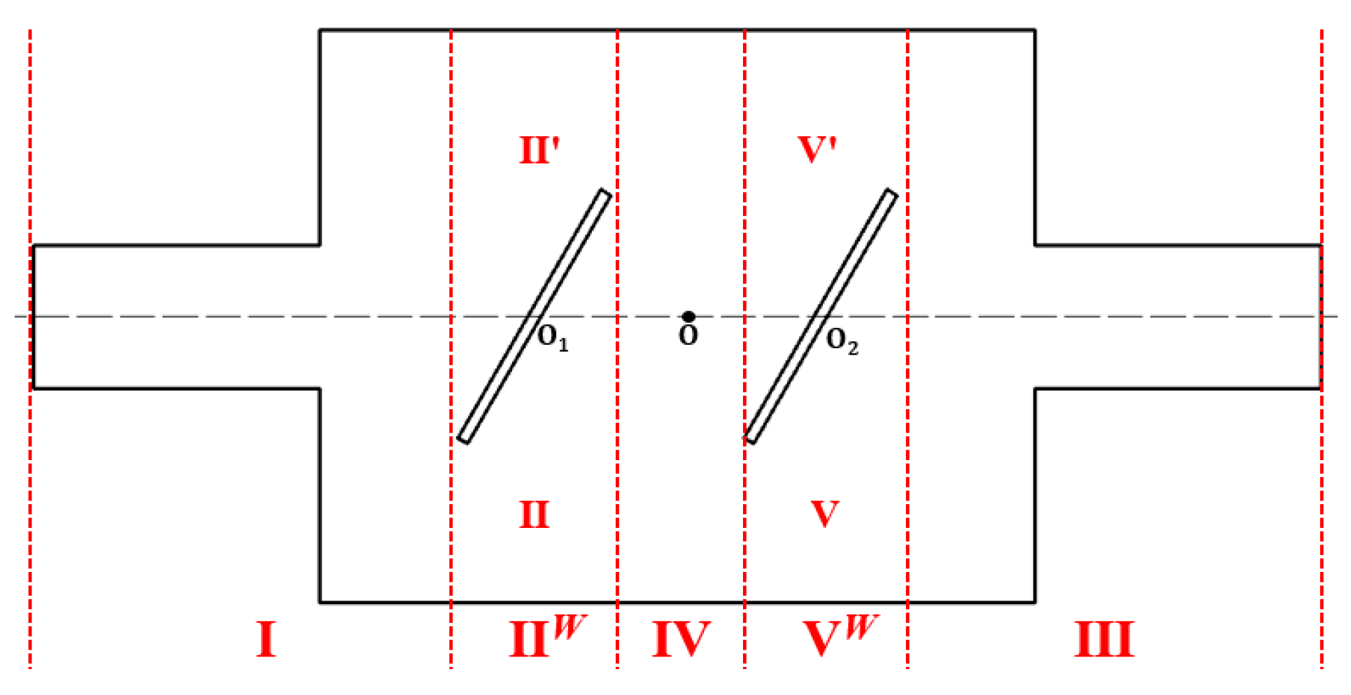
| —made of an expanding RDGC (II) and a shrinking RDGC (II′) | ||
| III | —made of two uniform ducts and one sudden contraction section |
| m | 0 | 1 | 2 | |
|---|---|---|---|---|
| n | ||||
| 0 | 0 | 857.5 | 1715.0 | |
| 1 | 1143.3 | 1429.2 | 2061.2 | |
| 2 | 2286.7 | 2442.2 | 2858.3 | |
| Type 1 | Case 1-0 | 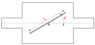 The REC with one baffle | lb = 0.50b, θ = 40° |
| Case 1-1 | lb = 0.50b, θ = 20° | ||
| Case 1-2 | lb = 0.50b, θ = 60° | ||
| Case 1-3 | lb = 0.30b, θ = 40° | ||
| Case 1-4 | lb = 0.40b, θ = 40° | ||
| Type 2a | Case 2a-0 |  The REC with double baffles distributed axially | lb = 0.50b, θ = 40° |
| Case 2a-1 | lb = 0.50b, θ = 20° | ||
| Case 2a-2 | lb = 0.50b, θ = 60° | ||
| Case 2a-3 | lb = 0.30b, θ = 40° | ||
| Case 2a-4 | lb = 0.40b, θ = 40° | ||
| Type 2t | Case 2t-0 | 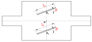 The REC with double baffles distributed transversely | lb = 0.50b, θ = 40° |
| Case 2t-1 | lb = 0.50b, θ = 20° | ||
| Case 2t-2 | lb = 0.50b, θ = 60° | ||
| Case 2t-3 | lb = 0.30b, θ = 40° | ||
| Case 2t-4 | lb = 0.40b, θ = 40° |
| Parameters | Values |
|---|---|
| Temperature | 24.5 °C |
| Relative humidity | 29.2% |
| Pressure | 101,300 Pa |
| Case 1-0 | Case 2a-0 | Case 2t-0 |
|---|---|---|
| 141 Pa | 140.2 Pa | 117.7 Pa |
Publisher’s Note: MDPI stays neutral with regard to jurisdictional claims in published maps and institutional affiliations. |
© 2022 by the authors. Licensee MDPI, Basel, Switzerland. This article is an open access article distributed under the terms and conditions of the Creative Commons Attribution (CC BY) license (https://creativecommons.org/licenses/by/4.0/).
Share and Cite
Sun, Y.; Qiu, Y.; Liu, L.; Zheng, X. Three-Dimensional Acoustic Analysis of a Rectangular Duct with Gradient Cross-Sections in High-Speed Trains: A Theoretical Derivation. Appl. Sci. 2022, 12, 5307. https://doi.org/10.3390/app12115307
Sun Y, Qiu Y, Liu L, Zheng X. Three-Dimensional Acoustic Analysis of a Rectangular Duct with Gradient Cross-Sections in High-Speed Trains: A Theoretical Derivation. Applied Sciences. 2022; 12(11):5307. https://doi.org/10.3390/app12115307
Chicago/Turabian StyleSun, Yanhong, Yi Qiu, Lianyun Liu, and Xu Zheng. 2022. "Three-Dimensional Acoustic Analysis of a Rectangular Duct with Gradient Cross-Sections in High-Speed Trains: A Theoretical Derivation" Applied Sciences 12, no. 11: 5307. https://doi.org/10.3390/app12115307
APA StyleSun, Y., Qiu, Y., Liu, L., & Zheng, X. (2022). Three-Dimensional Acoustic Analysis of a Rectangular Duct with Gradient Cross-Sections in High-Speed Trains: A Theoretical Derivation. Applied Sciences, 12(11), 5307. https://doi.org/10.3390/app12115307