Damage Detection in Wind Turbine Blades Based on an Improved Broad Learning System Model

Abstract

The research on damage detection in wind turbine blades plays an important role in reducing the risk of shut down in wind turbines. Rapid and accurate damage identification by using efficient detection models is the focus of the current research on damage detection in wind turbine blades. To solve the problems of the complex structure of the model and high time consumption in deep learning models, an improved broad learning system (BLS) model using the algorithm of chunking based on non-local means (NLMs) was proposed, which was called the CBNLM-BLS. The chunked, in-parallel accelerated integral image approach was used to optimize the NLM to speed up the BLS. Experiment results showed that the proposed model achieved a classification accuracy of 99.716%, taking 28.662 s to detect damage in the wind turbine blades. Compared with deep neural network models, such as ResNet, AlexNet and VGG-19, the proposed CBNLM-BLS had higher classification accuracy, shorter training time and less complex model construction and parameters. Compared with traditional BLSs, the CBNLM-BLS had less time complexity. It is of great significance to identify damage in wind turbine blades more efficiently.

1. Introduction

In recent years, the development and utilization of renewable energy has been highly valued by many countries. Wind energy is a new and renewable energy source with great value for exploitation and has become the fastest growing renewable energy source in the world. It is gradually occupying an important position in the global energy structure and is highly competitive with traditional energy sources. Figure 1 shows the global cumulatively installed wind power capacity and growth rate from 2001 to 2020, as compiled by the Global Wind Energy Council (GWEC) and Weber Consulting [1]. Over the last two decades, global wind power has grown rapidly. Cumulatively installed wind power capacity has increased from 24 GW to 743 GW, with a compound annual growth rate of over 20%. Since 2020, it has remained on track despite the impact of COVID-19. Wind turbines are moving towards being developed on a large scale, as the number of installed wind turbines grows. By 2030, the globally installed capacity of wind power will exceed 2000 GW [2]. Large wind turbines place higher demands on the safe and reliable operation of their components [3]. As size and power ratings increase, the analysis of support structures and blades subjected to wind loads become increasingly important [4].

Wind turbine blades are a crucial component for capturing wind energy. Wind turbine blades need to be manufactured from materials with excellent characteristics due to their working environment. Despite all the effort that has been put into the material of the blades, the surface is inevitably subject to various defects due to the constant exposure to storms, sand, lightning, rain and snow. The cost of wind turbine components accounts for around 20% of the overall installed cost [5], which is high. Wind turbines could suffer from varying degrees of damage during operation. If not repaired in time, this could have a serious impact on the cost control and output efficiency of wind power generation and could even cause serious accidents [6]. The prevention and identification of defects in the blades of wind turbines in advance could reduce the incidence of accidents and economic losses.

With the development of neural network technology, deep learning algorithms have received increasing attention from academic and industrial fields in the processing of images [7,8]. Xiyun Yang et al. [9] proposed a new convolutional neural network (CNN) model with the classifiers of migration learning and integrated learning to improve the accuracy of defect detection in the blades of wind turbines. Xu Donghua et al. [10] selected VGG-11 as a damage recognition model for wind turbine blades and used the algorithm of the alternating direction method of multipliers (ADMM) to compress the model to reduce the requirements on the hardware devices. Wen et al. [11] proposed a new CNN developed on the basis of the LeNet-5 neural network to detect the damage types in rotating machinery. A detection method combining a back propagation (BP) neural network and a support vector machine was proposed by Zhou as the machine classifier [12]. The experimental nature of deep learning methods usually requires a large amount of image data to provide the foundational support. The large amount of data and the slow running processes have become the biggest problems for deep learning.

The BLS was proposed by Philip Chen in 2017 [13,14]. It is regarded as the replacement for the deep learning structure. The problems of time consumption and complex structures in deep learning models are solved by the BLS. Chen proposed that convolutional and pooling operations should be used to improve the feature extraction capability of traditional BLSs for images to reduce the training time [15]. The intrinsic graph with the BLS (IGBLS) and the intrinsic penalty graph with the BLS (IPGBLS) have been proposed by Jin to further mine image features [16]. Zhao extended the BLS to semi-supervised learning for classification using a large number of unlabeled samples combined with the theory of manifold regularization to improve the accuracy of the model for image classification [17]. The graph convolutional broad network (GCB) proposed by Wang and Zhang has been used to explore the deep information of image structure to analyze data more effectively [18]. Up until now, the BLS has not been used for damage detection in wind turbine blades.

Although deep learning algorithms have been widely used in image processing, with the deepening of model structure, time complexity of back propagation is becoming higher and higher [19]. Deep learning algorithms also rely heavily on labelled images that are getting increasingly difficult to develop; therefore, it is necessary to develop a new model to better analyze images [20]. The CBNLM-BLS was proposed as a novel model based on the BLS and has been applied to damage detection in wind turbine blades in this work. The main contribution of this paper consists of the following two aspects.

On one side, to solve the problem of the low computational efficiency in NLMs, the method of improving NLMs using the chunked, in-parallel approach is proposed. It solved the problem of repeated calculations for finding the difference value of pixels pair by pair in the NLM. The use of chunked operations sped up the operation of the integral map, which, in turn, improved the overall operation efficiency of the NLM.

On the other side, to solve the problem of the poor generalization ability caused by little image data, the CBNLM-BLS-based damage detection for wind turbine blades was established. The proposed model had a single hidden layer structure, and the model performance could be improved only by adjusting the number of feature nodes and enhancement nodes. By calculating the pseudo-inverse of the feature nodes and enhancement nodes to the target value to calculate the weights, the training speed of the model was improved rapidly.

2. Mathematical Preliminaries

2.1. Non-Local Means

NLMs [21] are a novel denoising technique that was recently proposed. The method makes full use of the redundant information in an image, and is able to maintain the amount of detail in an image. The NLM uses mean-square error (MSE) to calculate the similarity of two neighborhood blocks. The rows and columns of the neighborhood blocks are the same. Assuming neighborhood blocks all consist of m rows and n columns, the MSE can then be calculated as follows (Equation (1)), where A(i, j) is the pixel value of point (i, j) in the neighborhood block centered on point A and B(i, j) is the pixel value of the point at the same position in the neighborhood block centered on point B.

$$MSE(A,B)=\frac{1}{mn}{\displaystyle \sum _{i=0}^{m-1}{\displaystyle \sum _{j=0}^{n-1}{\left(A\left(i,j\right)-B\left(i,j\right)\right)}^2}},$$

(1)

Let the image with noise be $v$ and the denoised image be $\tilde{u}$, the filter value of point A $\tilde{u}\left(A\right)$, namely the denoised image of A, can be obtained by the weighted average of the pixel values of all points in the search window, as is shown in Equation (2). $w\left(A,B\right)$ is the Gaussian weight of point A and any point B in the search window, which can be calculated by Equation (3), where the sum is calculated by Equation (4), and h is a smoothing parameter which is proportional to the standard deviation of the noise.

$$\tilde{u}(A)={\displaystyle \sum _{}w(A,B)v(B)},$$

(2)

$$w\left(A,B\right)=\frac{1}{sum}{e}^{-\frac{MSE(A,B)}{h^2}}$$

(3)

$$sum={\displaystyle \sum e^{-\frac{MSE(A,B)}{h^2}}}$$

(4)

2.2. Broad Learning System

The BLS was proposed by Philip Chen in 2017 [13]. As an alternative to deep network structures, the input data are first mapped to mapped features before being mapped to enhancement nodes. The output layer connects both the mapped feature layer and the enhancement node layer.

The data are transformed by a linear mapping function connecting the input weight matrices to obtain a mapping feature set. The mapped features are noted as $Z_i$, the ith set of mapped features, i = 1, 2, …, n, obtained after a linear mapping and activation function, i.e.,

$$Z_i={\varphi }_i(X{W}_{e_i}+{\beta }_{e_i}),i=1,2,\dots ,n,$$

(5)

where $X\in R^{a\times b}$ denotes the input sample data for model training, where the number of samples is a and the dimension of each sample is b. $W_{e_i}$ denotes the weight matrix of the ith feature node, the optimal input connection weight matrix obtained by sparse autoencoder fine-tuning. ${\varphi }_i$ is the activation function of the feature node. ${\beta }_{e_i}$ denotes the input layer to the mapping feature layer with $W_{e_i}$ being the corresponding bias matrix. The dimension of the weights $W_{e_i}$ determines the number of nodes in the $Z_i$ mapped feature group. To tackle the problems caused by randomness, a sparse autoencoder effectively reduces the linear correlation of newly generated feature nodes [22,23]. What makes the sparse feature matrix learning model attractive is that it can explore essential features [24,25]. The mapped feature group obtained by n transformations is denoted as follows:

$$Z^n=[Z_1,Z_2,Z_3,\dots ,Z_n],$$

(6)

The enhancement nodes are obtained from the mapped nodes by a nonlinear mapping and activation function transformation. Denote $H_j$ as the jth group of enhancement nodes, j = 1, 2, …, m, that is the following:

$$H_j={\xi }_j(Z^n{W}_{h_j}+{\beta }_{h_j}),j=1,2,\dots ,m,$$

(7)

where ${\xi }_j$ is the activation function of the enhancement node. $W_{h_j}$ denotes the random connection weight matrix of the jth group of mapped feature nodes to the enhancement node layer. ${\beta }_{h_j}$ denotes the jth group of bias matrices, and the group of enhancement nodes obtained by m transformations is denoted as follows:

$$H^m=[H_1,H_2,H_3,\dots ,H_m],$$

(8)

The mapped feature nodes together with the enhancement nodes are used as inputs for the BLS and is solved for the eigenvector using $Y=[Z^n|H^m]W^m$.

Where matrix $[Z^n|H^m]$ denotes the actual input to the BLS. $Y$denotes the eigenvector of the input. $W^m$denotes the matrix of weights connecting the input to the output layer of the system, which is solved by solving a ridge regression [26], as follows:

$$W^m={(\lambda I+A^{\top }A)}^{-1}{A}^{\top }Y,$$

(9)

where $A=[Z^n|H^m]$ denotes the actual input to the BLS. $\lambda$ denotes the regularization factor and $I$ denotes the unit matrix.

3. Damage Detection in Wind Turbine Blades Based on the CBNLM-BLS

In order to solve the problems of low operational efficiency of NLMs and the complex structure of deep neural networks [27], an improved model based on CBNLMs to accelerate the BLS was proposed in this paper. It was applied to the field of damage detection in wind turbine blades. To demonstrate the effectiveness of the proposed network for wind turbine blade damage detection and the simplicity of the model, this chapter compared it with existing mainstream methods in terms of classification capability as well as model structure.

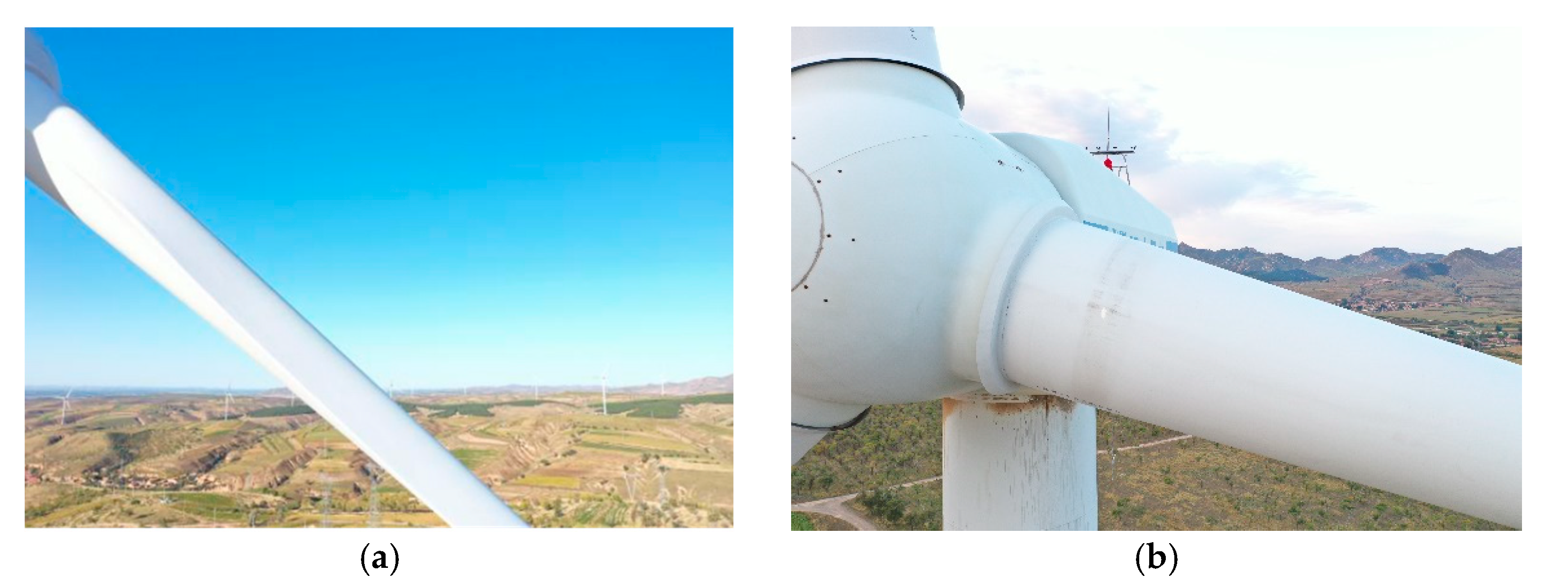
3.1. The Acquisition of Wind Turbine Blade Images

To develop a database containing cracked, normal wind turbine blades, multiple images were truncated using the region of interest (ROI) method on the images captured by the DJI UAV Royal Mavic 2. The database was then expanded by rotating, panning, adding noise, changing brightness, contrast, etc. The final 741 images of the wind turbine blades were generated. All images collected were canonically processed and were 256 × 256 in size. The image dataset was divided into a training set and a test set on a scale of 3:1. The details of the dataset’s categories are shown in

Table 1. The details of the image dataset.

	The Number of Images	Images with Damage	Images without Damage
Training set	556	266	290
Testing set	185	88	97
Total	741	354	384

. Two collected image samples of wind turbine blades are shown in Figure 2.

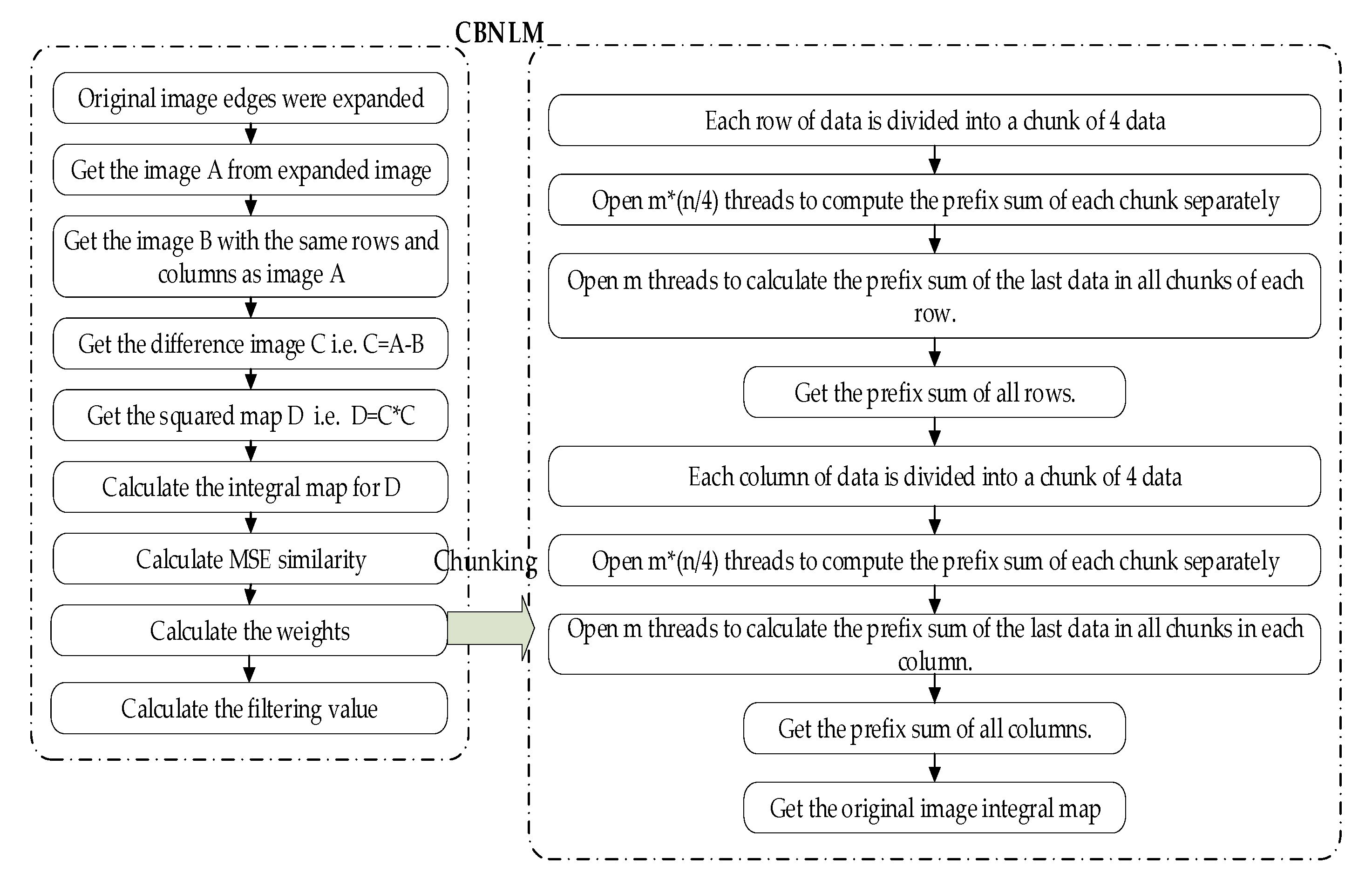
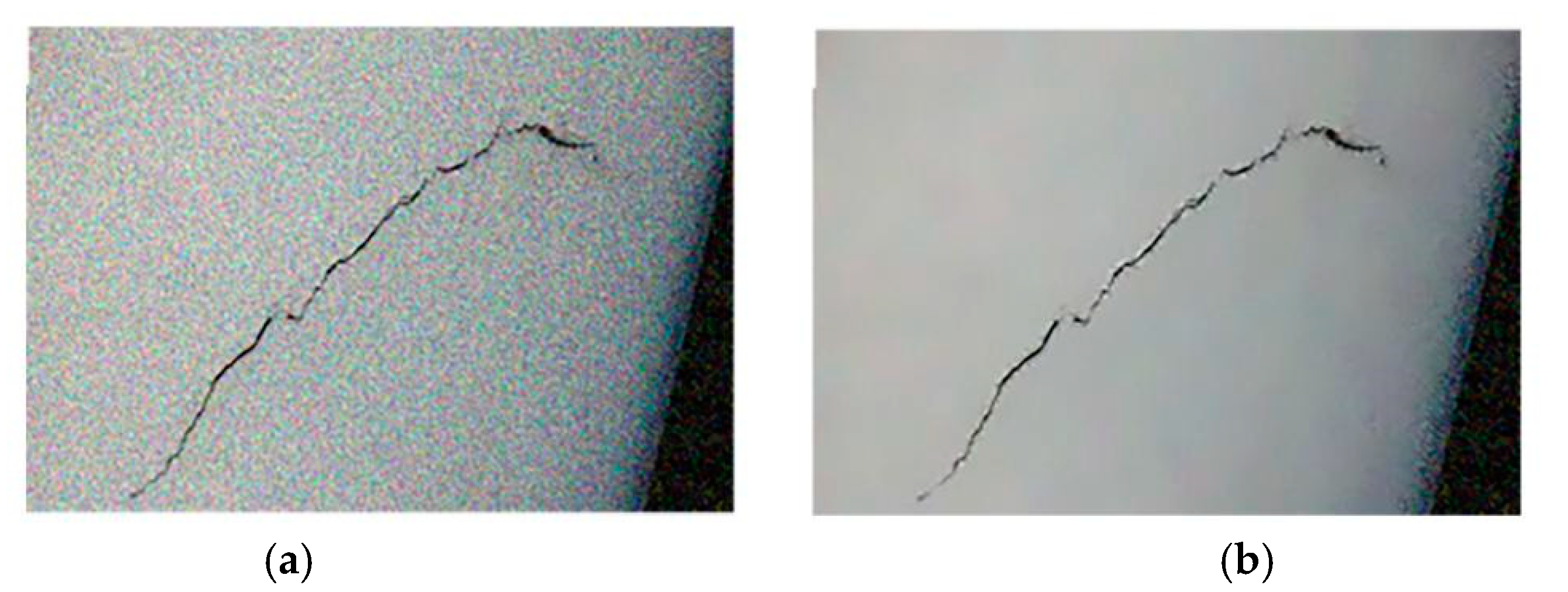
3.2. The CBNLM for Pre-Processing of Images

Images are inevitably affected by noise during acquisition, storage, recording and transmission, which reduces the contrast of the image and seriously affects its application [28]. In image pre-processing algorithms, the method of mean filter denoising loses feature information in the image, tends to blur the image and is powerless against pretzel noise [29,30]. The above problems can be solved by NLMs. However, NLMs have the problem of a long running time [31]. Its main time-consuming point is the frequent calculation of the mean square error (MSE) of two patches. This paper proposed the use of a chunked, in-parallel approach to speed up the computation of the MSE for two patches, which improved the computational speed of the NLM.

It is well known that for an image the prefix sums of all its rows are calculated separately to obtain the prefix-sum image. The prefix sum of all columns is then calculated separately for the image of the row prefix sum to obtain the integral image. The flowchart of the complete CBNLM is shown in Figure 3. The critical process of the CBNLM for m-row and n-column images consisted of the following nine steps.

Step 1: Each row of data is divided into four data blocks, and m × (n/4) threads are opened. Each thread computes the prefix sum of the four data blocks, and all threads are computed in parallel.

Step 2: Each thread corresponds to a row of data and is responsible for calculating the prefix sum of the last data block in all the small blocks in that row, opening m threads.

Step 3: A total of m × (n/4) threads are opened, each corresponding to a small block. For each row, the number in each chunk (except the last number) is added to the last number of its previous chunk to obtain the prefix sum of all rows, starting with the second chunk.

Step 4: Each column of data is divided into chunks of four data blocks each and (m/4) × n threads are opened. Each thread computes the prefix sum of the four data blocks in a chunk, and all threads are computed in parallel.

Step 5: A total of n threads are opened. Each thread corresponds to a column of data and is responsible for calculating the prefix sum of the last data in all the small blocks in that column.

Step 6: A total of (m/4) × n threads are opened. Each thread corresponds to one chunk. For each column, starting with the second chunk, the number in each chunk (except the last number) is added to the last number of its previous chunk to obtain the prefix sum of all columns. This is the integral image of the original image.

Step 7: Once the integration map is obtained, the neighborhood block area is acquired according to the position of the current point to be filtered on the integration map. The average of the pixel values of all points in the neighborhood block area is quickly calculated, which is the MSE similarity.

Step 8: The Gaussian weights of the points to be filtered and any point in the search window are calculated from the MSE similarity of the neighborhood blocks.

Step 9: The filter value is calculated as a weighted average of the pixel values of all points within the search window.

The images before and after the CBNLM are shown in Figure 4.

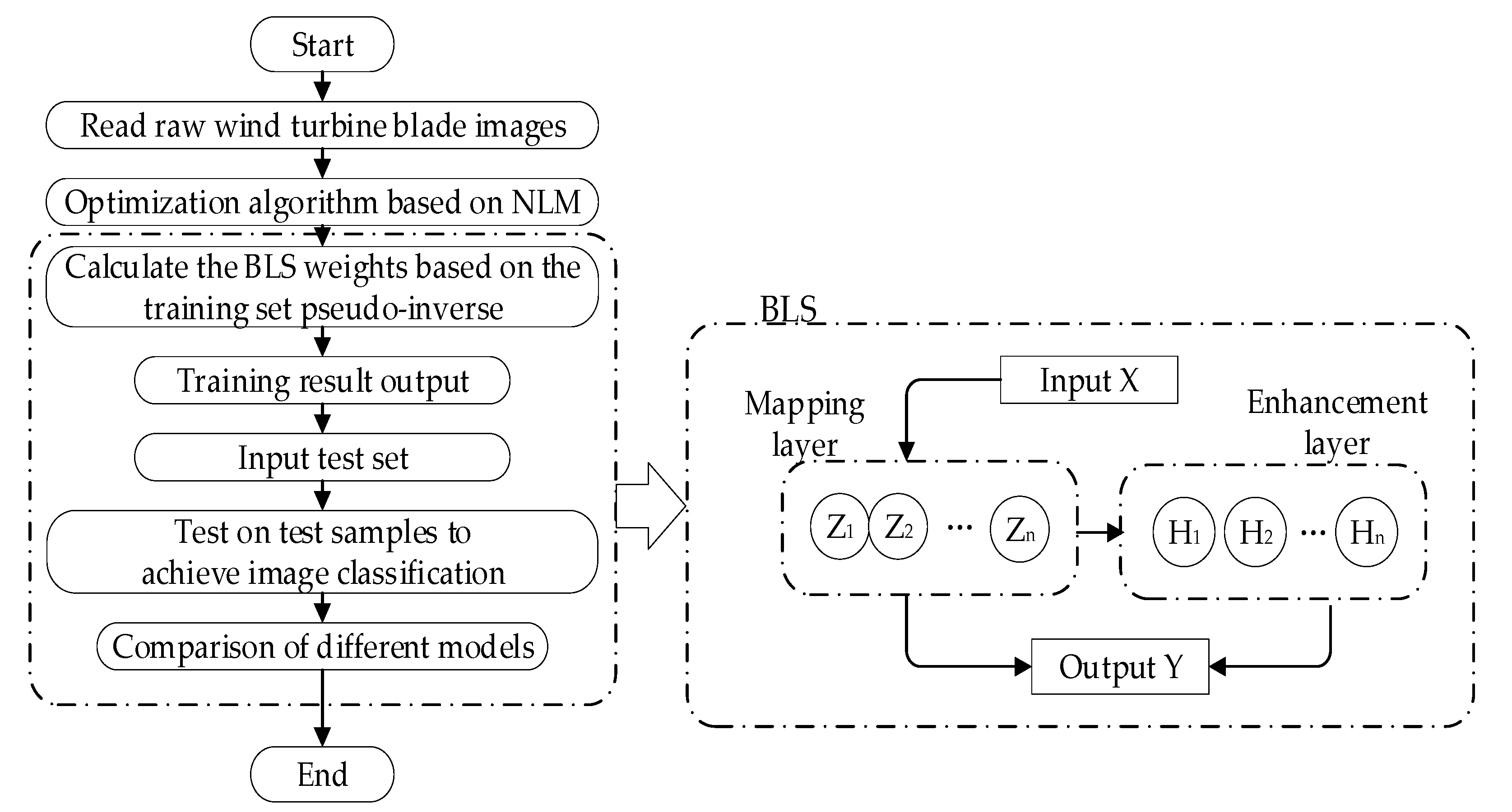
3.3. Construction of the CBNLM-BLS

The CBNLM-BLS performs feature extraction on input data X. The input data are mapped into multiple feature nodes, which are classified as mapped features $Z_1,\dots ,Z_n$ in that part of the data. $Z_1,\dots ,Z_n$ are first multiplied by a set of random weights, $W$, and then biased. The activation function is processed as the output of the enhancement node layer, noted as $H_1,\dots ,H_m$. Finally, $Z_1,\dots ,Z_n$ mixed with $H_1,\dots ,H_m$ is noted as $A=\left[Z | H\right]$. The output is noted as $Y={AW}_m$. The core of the CBNLM-BLS is to find the pseudo-inverse of the feature nodes and enhancement nodes to the target value. The CBNLM-BLS is constructed in three steps as follows: generation of feature nodes, generation of enhancement nodes and finding the pseudo-inverse. The input layer data set is noted as $\left(s\times f\right)\times H_1$, where $s$ denotes the number of samples and $f$ denotes the number of features. For two-dimensional images, the code pulls it into a one-dimensional vector; the feature node layer contains $N_1$ feature node windows, each containing $N_2$ feature nodes and the enhancement layer contains $N_3$ enhancement nodes.

The construction of the CBNLM-BLS consists of the following steps.

1.

The generation of feature nodes.

A mapping of input data to feature nodes is created. The Z-score normalization is carried out for $H_1^{}$ to ensure that the input data have been normalized to between 0–1 of its expansion, making it $H_{1\left[s\times \left(f+1\right)\right]}$. In order to generate feature nodes, bias terms can be added directly by matrix operations.

Feature nodes are generated for each window. An $\left(f+1\right)\times N_2$-dimensional random weight matrix, $W_e$, is generated. The features of each sample are convolved and biased once with random weights to obtain the new features, $A_1=H_1^{}\times W_e$. The new features are sparsely represented and normalized, resulting in a window of feature nodes T₁.

$N_2$ feature nodes are generated for each of the $N_1$ feature windows. Each feature node is an $s$-dimensional feature vector. For the whole network, the feature node matrix $y$ is a matrix of dimension $s\times \left(N_1\times N_2\right)$.

2.

Enhancement nodes are generated.

The CBNLM-BLS can make use of enhancement nodes to complement the random feature nodes, which are linear. The enhancement nodes are introduced with the aim of enhancing the non-linear elements in the network.

A mapping of feature nodes to enhancement nodes is created. As with the feature nodes, the feature node matrix $y$ is first normalized and expanded to obtain $H_2$. Unlike the feature node, the coefficient matrix of the enhancement node is not a random matrix, but is a random matrix normalized orthogonally. The coefficient matrix of the enhancement nodes, $W_h$, can be $N_1\times N_2>N_3$ expressed as an $N_1\times N_2\times N_3$ dimensional orthogonal normalized random matrix, which allows the feature nodes to be mapped to a higher dimensional subspace through non-linearity, making the network more expressive and provides an ‘augmentation’ effect. Afterwards, activation operations are performed on the augmented nodes to maximize the activation of the features expressed by the augmented nodes to generate T₂.

T₃ is the final input of the generated network. Compared with the feature nodes, the enhancement nodes did not require a sparse representation or window iterations. Although the iterations of orthogonalization consumed some computational time, the time to add augmented nodes was often less than adding feature nodes, and the final input T₃ of the network can be expressed as ${\left[y,T_2\right]}^T$, where each sample feature dimension is $N_1\times N_2+N_3$.

3.

Pseudo-inversion is sought.

Let $yy$ be the output value of the network, i.e., $yy=T_3\times W$. Then the pseudo-inverse matrix is $W={\left(T_3^T\times T_3^{}+C\times I^{N_1\times N_2+N_3}\right)}^{-1}\left(T_3^T\times Y\right)$, where $C$ is the regular term parameter and $Y$ is the training set label. At this point the input and weights of the whole network is trained. Finally, the network is used $yy=T_3\times W$ to make predictions.

The flowchart of the proposed wind turbine blade damage identification model based on the CBNLM-BLS is shown in Figure 5 below.

3.4. Results and Discussion

All experiments were completed on a Windows 10 computer system equipped with Inter 1.70 GHz and 16 GB of RAM by using pyCharm 2021.

To demonstrate the effectiveness and model simplicity of CBNLM-BLS for wind turbine blade damage detection, the algorithms in this paper were compared with existing mainstream methods in terms of classification capability and model structure, ResNet101 [32], VGG19 [33] and AlexNet [34]. The deep learning network hyperparameters involved were tuned based on backpropagation. The initial learning rate was set to 10⁻⁵ and the activation functions were all RELU. In the CBNLM-BLS, the regularization parameter for ridge regression was set to 10⁻⁸. The relevant parameters, ${\omega }_{e_i}$ and ${\beta }_{e_i}$, were extracted from a standard unified distribution of [−1, 1] and the tansig function was chosen for the enhancement node layer.

A line chart for the variation in damage recognition accuracy with the number of iterations for each neural network algorithm is shown in Figure 6. It could be seen from the figure that the accuracies of ResNet, VGG19 and AlexNet did not increase with the increase in iterations, but remained unchanged within a certain range. Different from other deep networks, the accuracy of the CBNLM-BLS was changed by adjusting the number of nodes. The horizontal coordinate in Figure 6d represents the number of increases of enhancement nodes. The figure shows that the accuracy of the CBNLM-BLS decreased with the increase in the number of nodes. This was because the enhancement nodes that were converted were sufficient to extract enough features to obtain an accurate classification result after the images were fed into the model.

In addition to the comparison in terms of accuracy, the four metrics of precision and recall as well as F1 score and time were introduced. For the problem of two kinds of classification for damage detection in wind turbine blades, the image samples were divided into cases of true positive (TP), false positive (FP), true negative (TN) and false negative (FN) according to the combination of actual categories and predicted categories. A confusion matrix of classification results is shown in

Table 2. Explanatory table for evaluation indicators.

Actual Categories	Predicted Categories
	Positive	Negative
Positive	TP	FN
Negative	FP	TN

. The results of the comparison of the different models are shown in

Table 3. Comparison of the classification results in different classification algorithms for wind turbine blade damage.

Algorithm	Accuracy (%)	Precision (%)	Recall (%)	F1_Score (%)	Times (s)
ResNet	81.035	94.444	37.778	53.968	35,939
AlexNet	95.700	81.818	100	90.000	11,898
VGG19	82.609	82.609	100	90.476	13,063
BLS	99.107	100	98.276	99.131	51.126
CBNLM-BLS	99.716	98.630	100	99.310	28.662

.

The accuracy indicated the number of correct samples predicted as a proportion of the total sample.

$$\mathrm{Accuracy}=\frac{\mathrm{TP}+\mathrm{TN}}{\mathrm{TP}+\mathrm{TN}+\mathrm{FP}+\mathrm{FN}},$$

(10)

The precision represented the probability that all samples with a positive prediction were actually positive.

$$\mathrm{Precision}=\frac{\mathrm{TP}}{\mathrm{TP}+\mathrm{FP}},$$

(11)

Recall represented the probability that of samples that were actually positive were predicted to be positive.

$$\mathrm{Recall}=\frac{\mathrm{TP}}{\mathrm{TP}+\mathrm{FN}},$$

(12)

F1_Score was a weighted harmonic mean of precision and recall.

$$\mathrm{F}1\text{\_}\mathrm{score}=\frac{2\mathrm{Precision}\times \mathrm{Recall}}{\mathrm{Precision}+\mathrm{Recall}},$$

(13)

As can be seen from Table 3, in the experiments for damage detection in wind turbine blades, the CBNLM-BLS model proposed in this work had the highest classification accuracy of 99.716%. While the BLS, ResNet101, AlexNet and VGG19 algorithms had accuracies of 99.107%, 81.0%, 95.7% and 82.6%, respectively. Compared with other models, the BLS model had the highest precision of 100%. The precision of the CBNLM-BLS was 98.63%, which was slightly lower than that of the BLS. Although the recall rate of the CBNLM-BLS was the same as AlexNet and VGG19, the accuracy of CBNLM-BLS was better than other models. The F1-score value of CBNLM-BLS was bigger than the other four, indicating that the classification effect of the model was the best. The two algorithms of the BLS and the CBNLM-BLS were both much faster than the other three deep neural networks, indicating that they could overcome the weakness of the large time consumption and the high complexity of structure in deep learning neural networks such as ResNet, AlexNet and VGG-19. Compared with the traditional BLS, the training time of the CBNLM-BLS was shorter, at 28.662 s. It revealed that by using chunked parallelism, the computing speed of the CBNLM-BLS algorithm was greatly improved and it had less time complexity than the BLS.

Figure 7 shows the structures of ResNet, CBNLM-BLS, AlexNet and VGG19, respectively. The structural diagrams show that the CBNLM-BLS had no layer-to-layer coupling, no multi-layer connections, no more parameters to save and no need to update the weights using gradient descent.

Parametric analysis of the proposed CBNLM-BLS for damage detection in wind turbine blades is shown in

Table 4. Comparison of the results of the CBNLM-BLS for damage images of the wind turbine blade on the collected image dataset when taking different parameters.

N1	N2	N3	Accuracy (%)	Times (s)
10	10	100	99.639	28.301
		150	99.639	27.211
		200	99.819	27.327
5	10	50	99.097	14.543
10			99.639	27.891
15			99.639	41.060
10	5	50	99.278	14.078
	10		99.639	27.327
	15		99.639	41.752

, when the network parameters took different values, where N₁ denoted the number of windows, N₂ denoted the number of nodes per window and N₃ denoted the number of enhancement nodes.

As can be seen in Table 4, the accuracy of the CBNLM-BLS did not increase with the increase in N₃, and the training time changed in a certain range when N₁ and N₂ were set to be unchanged. The accuracy did not increase with the increase in N₁, and the training time increased accordingly when N₂ and N₃ were set to be unchanged. When N₁ and N₃ remain unchanged, the training time increased with the increase in N₂, but the accuracy did not increase with the increase in N₂, indicating that the classification accuracy of the random broad learning network, in a certain range, and the increase in N₁, N₂ and N₃ would make the extracted features richer and would obtain the best number of features in that range; thus, getting a higher classification. At the same time, as the nodes increased, the time also increased.

The dimensionality of the CBNLM-BLS parameters $W$ could be found to be a matrix of dimensionality $\left(N_1\times N_2+N_3,n\right)$, meaning that it was independent of the number of samples, s, in the training set. This implied that the feature nodes and augmentation nodes were generated according to the training steps and then used $yy=T_3\times W$ to make predictions, except that the feature nodes were generated according to the previous normalization criteria when they were generated. After training was complete, the only parameters that needed to be saved were in fact $W$ and the normalization method. Compared to deep learning algorithms, the CBNLM-BLS had fewer parameters and the training time was greatly reduced.

4. Conclusions

A novel CBNLM-BLS model for damage detection in wind turbine blades was proposed in this work. It could overcome the weakness of large time consumption and high complexity of structure in deep learning neural networks such as ResNet, AlexNet and VGG-19. Compared with the traditional BLS model, the CBNLM-BLS had less time complexity due to the use of chunked parallelism. Comparison experiment for damage detection of wind turbine blades was performed and it showed that the proposed CBNLM-BLS had the best performance and achieved a classification accuracy of 99.716% and took 28.662 s.

Future work would be concentrated on further validation of the CBNLM-BLS model and its application for real time and online damage detection in wind turbine blades.

References

1. Data Interpretation: Analysis of Global Wind Power Installed Capacity Growth Trend from 2001 to 2020. Available online: https://www.sohu.com/a/496115969_100158378?spm=smpc.author.fd-d.4.1651547430984GFPQYRM (accessed on 20 October 2021).
2. Global Wind Energy Council. GWEC|Global Wind Report 2021; Global Wind Energy Council: Brussels, Belgium, 2021. [Google Scholar]
3. Lu, J.Q.; Mou, S.X. Advances in leading edge protection technology of wind turbine blades. J. Gla. Fiber. Reinf. Plast. 2015, 7, 91–95. [Google Scholar]
4. Yuan, C.; Li, J. Investigation on the Effect of the Baseline Control System on Dynamic and Fatigue Characteristics of Modern Wind Turbines. Appl. Sci. 2022, 12, 2968. [Google Scholar] [CrossRef]
5. Wang, Z.G.; Yang, B. Advances in online monitoring technology for wind turbine blades under operating conditions. J. Eng. Ther. Energy Power 2017, 32, 1–5. [Google Scholar]
6. Skrimpas, G.A.; Kleani, K. Detection of icing on wind turbine blades by means of vibration and power curve analysis. Wind Energy 2016, 19, 1819–1832. [Google Scholar] [CrossRef]
7. Yeum, C.M.; Choi, J. Automated region-of-interest localization and classification for vision-based visual assessment of civil infrastructure. Struct. Health Monit. 2019, 18, 675–689. [Google Scholar] [CrossRef]
8. Lenjani, A.; Dyke, S.J. Towards fully automated post-event data collection and analysis: Pre-event and post-event information fusion. Eng. Struct. 2020, 208, 109884. [Google Scholar] [CrossRef] [Green Version]
9. Yang, X.; Zhang, Y.; Lv, W.; Wang, D. Image recognition of wind turbine blade damage based on a deep learning model with transfer learning and an ensemble learning classifier. Renew. Energy 2021, 163, 386–397. [Google Scholar] [CrossRef]
10. Xu, D.; Wen, C.B. Wind turbine blade surface inspection based on deep learning and UAV-taken images. J. Renew. Sust. Energy 2019, 11, 053305. [Google Scholar] [CrossRef]
11. Wen, L.; Li, X.Y. A New Convolutional Neural Network-Based Data-Driven Fault Diagnosis Method. IEEE Trans. Ind. Electron. 2017, 65, 5990–5998. [Google Scholar] [CrossRef]
12. Zhou, S.T.; Li, Y.Y. Optical Inspection Technology of metal surface defects based on machine vision. Nondestruct. Test. 2020, 42, 39–44. [Google Scholar]
13. Chen, C.; Liu, Z. Broad Learning System: An Effective and Efficient Incremental Learning System without the Need for Deep Architecture. IEEE Trans. Neural Netw. Learn. Syst. 2018, 29, 10–24. [Google Scholar] [CrossRef]
14. Chen, C.P.; Liu, Z. Broad learning system: A new learning paradigm and system without going deep. In Proceedings of the 2017 32nd Youth Academic Annual Conference of Chinese Association of Automation, Hefei, China, 19 May 2017. [Google Scholar]
15. Chen, C.P.; Liu, Z. Universal approximation capability of broad learning system and its structural variations. IEEE Trans. Neural Netw. Learn. Syst. 2018, 30, 1191–1204. [Google Scholar] [CrossRef]
16. Jin, J.; Liu, Z.L. Discriminative graph regularized broad learning system for image recognition. Sci. China Inf. Sci. 2018, 61, 1–14. [Google Scholar] [CrossRef]
17. Zhao, H.; Zheng, J.J. Semi-supervised broad learning system based on manifold regularization and broad network. IEEE Trans. Circuits Syst. I Regul. Pap. 2020, 67, 983–994. [Google Scholar] [CrossRef]
18. Zhang, T.; Wang, X.H. GCB-Net: Graph convolutional broad network and its application in emotion recognition. IEEE Trans. Affect. Comput. 2019, 13, 379–388. [Google Scholar] [CrossRef]
19. Guha, R.; Das, N. Devnet: An efficient cnn architecture for handwritten devanagari character recognition. Int. J. Pattern Recognit. Artif. Intell. 2020, 34, 2052009. [Google Scholar] [CrossRef]
20. Jiao, L.; Zhao, J. A survey on the new generation of deep learning in image processing. IEEE Access 2019, 7, 172231–172263. [Google Scholar] [CrossRef]
21. Zhan, Y.; Wu, J.; Ding, M.; Zhang, X. Nonlocal means image denoising with minimum MSE based decay parameter adaptation. IEEE Access 2019, 7, 130246–130261. [Google Scholar] [CrossRef]
22. Gong, M.; Liu, J. A Multiobjective Sparse Feature Learning Model for Deep Neural Networks. IEEE Trans. Neural Netw. Learn. Syst. 2017, 26, 3263–3277. [Google Scholar] [CrossRef]
23. Tibshirani, R. Regression shrinkage and selection via the lasso: A retrospective. J. R. Stat. Soc. 2011, 73, 267–288. [Google Scholar] [CrossRef]
24. Boyd, S.; Parikh, N. Distributed Optimization and Statistical Learning via the Alternating Direction Method of Multipliers. Found. Trends Mach. Learn. 2010, 3, 1–122. [Google Scholar] [CrossRef]
25. Yang, W.; Gao, Y. MRM-Lasso: A Sparse Multiview Feature Selection Method via Low-Rank Analysis. IEEE Trans. Neural Netw. Learn. Syst. 2017, 26, 2801–2815. [Google Scholar] [CrossRef] [PubMed] [Green Version]
26. Hoerl, A.E.; Kennard, R.W. Ridge Regression: Biased Estimation for Nonorthogonal Problems. Technometrics 2012, 12, 80–86. [Google Scholar]
27. Wu, R.T.; Singla, A. Pruning deep convolutional neural networks for efficient edge computing in condition assessment of infrastructures. Comput. Civ. Infrastruct. Eng. 2019, 34, 774–789. [Google Scholar] [CrossRef]
28. Mafi, M.; Martin, H. A comprehensive survey on impulse and Gaussian denoising filters for digital images. Signal Process. 2019, 157, 236–260. [Google Scholar] [CrossRef]
29. Jain, P.; Tyagi, V. A survey of edge-preserving image denoising methods. Inf. Syst. Front. 2016, 18, 159–170. [Google Scholar] [CrossRef]
30. Mafi, M.; Rajaei, H. A robust edge detection approach in the presence of high impulse noise intensity through switching adaptive median and fixed weighted mean filtering. IEEE Trans. Image Process. 2018, 27, 5475–5490. [Google Scholar] [CrossRef]
31. Cai, B.; Liu, W. An improved non-local means denoising algorithm. Pattern Recognit. Artif. Intell. 2016, 29, 1–10. [Google Scholar]
32. He, K.; Zhang, X. Identity Mappings in Deep Residual Networks; Springer: Cham, Switzerland, 2016; pp. 630–645. [Google Scholar]
33. Simonyan, K.; Zisserman, A. Very Deep Convolutional Networks for Large-Scale Image Recognition. arXiv 2014, arXiv:1409.1556. [Google Scholar]
34. Krizhevsky, A.; Sutskever, I. ImageNet Classification with Deep Convolutional Neural Networks. Adv. Neural Inf. Process. Syst. 2012, 25, 1097–1105. [Google Scholar] [CrossRef]
Figure 1. Global cumulatively installed wind power capacity and rate of growth in 2001–2020 (GW, %).
Applsci 12 05164 g001
Figure 2. The collected images of wind turbine blades. (a) A wind turbine blade without damage; (b) a wind turbine blade with damage.
Applsci 12 05164 g002
Figure 3. Flowchart of the complete CBNLM.
Applsci 12 05164 g003
Figure 4. The image before and after the CBNLM. (a) The image before the CBNLM; (b) the image after the CBNLM.
Applsci 12 05164 g004
Figure 5. Flowchart of damage detection in wind turbine blades based on the CBNLM-BLS.
Applsci 12 05164 g005
Figure 6. Line chart of model accuracy variation with number of iterations. (a) Line chart of ResNet accuracy variation with number of iterations; (b) line chart of VGG19 accuracy variation with number of iterations; (c) line chart of AlexNet accuracy variation with number of iterations; (d) line chart of CBNLM-BLS accuracy variation with number of nodes.
Applsci 12 05164 g006
Figure 7. Structure of models. (a) Structure of ResNet; (b) structure of the CBNLM-BLS; (c) structure of VGG19; (d) structure of AlexNet.
Applsci 12 05164 g007