Abstract
Knowledge about crop type distribution is valuable information for effective management of agricultural productivity, food security estimation, and natural resources protection. Algorithms for automatic crop type detection have great potential to positively influence these aspects as well as speed up the process of crop type mapping in larger areas. In the presented study, we used 14 Sentinel-2 images to calculate 12 widely used spectral vegetation indices. Further, to evaluate the effect of reduced dimensionality on the accuracy of crop type mapping, we utilized principal component analysis (PCA). For this purpose, random forest (RF)-supervised classifications were tested for each index separately, as well as for the combinations of various indices and the four initial PCA components. Additionally, for each RF classification feature importance was assessed, which enabled identification of the most relevant period of the year for the differentiation of crop types. We used 34.6% of the ground truth field data to train the classifier and calculate various accuracy measures such as the overall accuracy (OA) or Kappa index. The study showed a high effectiveness of the Modified Chlorophyll Absorption in Reflectance Index (MCARI) (OA = 86%, Kappa = 0.81), Normalized Difference Index 45 (NDI45) (OA = 85%, Kappa = 0.81), and Weighted Difference Vegetation Index (WDVI) (OA = 85%, Kappa = 0.80) in crop type mapping. However, utilization of all of them together did not increase the classification accuracy (OA = 78%, Kappa = 0.72). Additionally, the application of the initial three components of PCA allowed us to achieve an OA of 78% and Kappa of 0.72, which was unfortunately lower than the single-index classification (e.g., based on only NDVI45). This shows that dimensionality reductions did not increase the classification accuracy. Moreover, feature importance from RF indicated that images captured from June and July are the most relevant for differentiating crop types. This shows that this period of the year is crucial to effectively differentiate crop types and should be undeniably used in crop type mapping.
1. Introduction
Taking into account the farm-to-fork strategy and the continuous progression of climate change and consequent changes in biodiversity, as well as increasing population growth, it is necessary to increase agricultural productivity to ensure food security and help protect natural resources. To address these challenges, information about the type of crops is important. However, capturing information about the crop types cultivated in a specific study area is challenging, because in many cases it mostly depends on farmers’ declarations, reports provided to the specific agricultural national agencies, and field investigations. Moreover, gathering this information in large spatial areas, e.g., in areas of communes or provinces, and storing it as a spatial database is labor-intensive and time-consuming. In Poland, information about crop types is quantitatively provided to the Agency for Restructuring and Modernization of Agriculture (ARMA) [1] by farmers’ declarations, omitting information on its spatial distribution. The availability of free remote sensing data from the Copernicus Programme has opened new avenues for studying automatic approaches for remote and automatic crop type mapping. This automatic detection, which will provide quantitative and spatial information on the type of crop cultivated in specific regions, can help to increase agricultural productivity and to monitor food production to a great extent [2].
In the literature, numerous examples of remote sensing applications can be found for crop type detection, including optical satellite data [3,4,5], SAR data [6,7], and data captured from unmanned aerial vehicles [8,9]. Moreover, some authors have utilized integrated approaches based on SAR as well as optical satellite images [2,10,11] or even Google Street View photographs for crop type detection [12]. However, optical time series data (OTSD) have been proven to be efficient for crop mapping over many years, because the phenological evolution of each crop produces a unique temporal profile of reflectance and spectral indexes [13]. For crop type mapping, some researchers have utilized a specific spectral index calculated from multitemporal satellite data [14,15], whereas others utilized many spectral indexes calculated from one image [16] or many spectral indices calculated from many multitemporal images [5,17]. In the literature, there are also studies based on reflectance information without the calculation of any spectral indices [13]. For all of these various input data, different methods have been utilized, including machine learning and deep learning techniques, which have been widely applied recently [18,19,20]. Additionally, considering that many vegetation indices are calculated from the same spectral bands with different mathematical formula, these indexes are correlated. Therefore, scientists have attempted to synthetize information included in this correlated vegetation indices by using various approaches such as feature selection via machine learning approaches [21,22] or by applying Principal Component Analysis (PCA), which allows to reduce redundant information within correlated variables [22,23,24]. However, various scientists report various effects on accuracy by applying PCA. Authors of [22] reported that models with the PCA-based features selection perform even worse than no feature selection. In contrary, [24] showed that Support Vector Machine classification with feature extraction (PCA) on individual image dates produced the most accurate classification (96.2%). Therefore, additional evaluation of this aspect is needed.
Considering these various approaches, the question arises whether a wider number of spectral indexes helps increase the accuracy of automatic crop detection and which of these indexes are the most valuable for crop mapping. Therefore, the main objective of the study was to evaluate which of the spectral indexes were the most valuable for detection of specific plant types in our study area, which was mostly cultivated with maize and winter wheat. Moreover, considering that vegetation indices are correlated with each other, principal component analysis (PCA) enables a reduction in redundant information between features. Therefore, the secondary goal of this study was to evaluate whether dimensionality reduction within indices will influence the accuracy of crop mapping. Furthermore, random forest enables the evaluation of feature importance; thus, the additional goal of this study was to evaluate the importance of the Sentinel-2 acquisition dates on crop differentiation. As an experimental test site, we selected an agricultural area close to the town of Jelcz-Laskowice in Poland, utilizing the random forest classification of 14 Sentinel-2 images and 12 vegetation indices.
2. Automatic Crop Type Mapping Using Spectral Indices
The Normalized Difference Vegetation Index (NDVI) is widely used for crop type detection. For example, Gumma et al., (2020) [15] evaluated the mapping of winter croplands and corresponding cropping patterns by utilizing NDVI and a spectral matching technique (SMT) for 16 multi-temporal Sentinel-2 data values and unsupervised classification. They achieved Kappa coefficients between 0.64 and 0.74 for these three various districts. Similarly, Heupel et al., (2018) [14] used a progressive classification algorithm based on the phenological development of plants and the corresponding reflectance characteristics and NDVI. They processed 36 and 47 multitemporal satellite images for the year of 2015 and 2016 from four sensors (Landsat-7 and -8, Sentinel-2A, and RapidEye) and achieved overall accuracy (OA) of 89.49% and 77.19% for 2015 and 2016, respectively. The lower performance for the year 2016 was mostly associated with adverse weather conditions.
In contrast, Zhang et al., (2020) [5] used eight multi-temporal Sentinel-2 data and five various spectral indices to analyze the performance of the temporal and spectral features used in machine-learning-based classification methods. Among the spectral indexes, they utilized NDVI as the well as the Perpendicular Moisture Index (PMI), Normalized Differential Senescent Vegetation Index (NDSVI), Normalized Difference Residue Index (NDRI), and Normalized Differential Tillage Index (NDTI). The resulting OA was between 95.92% and 97.85% and the Kappa value was between 0.93 and 0.96 for various machine learning methods. Additionally, Mestre-Quereda et al., (2020) [17] used three vegetation indices that incorporated the NIR band (NDVI, GDVI: Green Normalized Difference Vegetation Index; NDRE: Normalized Difference Red Edge Index) derived from RapidEye images for crop type classification. Their goal was to investigate the potential use of these indices on crop type classification and the effect of each index on the accuracy of the Support Vector Machine classification accuracy. The use of three vegetation indices resulted in a classification accuracy of 87.46% and a Kappa coefficient of 0.85, which proved to be higher than the classification accuracy of any dual combination of these three vegetation indices. Additionally, single-band classification of each index provided OAs between 57.84% and 63.42% and Kappa coefficients between 0.47 and 0.58, which clearly shows that the utilization of many spectral indices increases the final accuracy.
Furthermore, Kobayashi et al., (2020) [16] calculated 91 spectral indices from one cloudless Sentinel-2A MSI image and evaluated their performance in identifying each type of crop. For image classification, a stratified random sampling approach was applied to select the fields used for modeling (50%), hyperparameter tuning (25%), and evaluation (25%) of the classification to prevent overfitting. The study showed that the use of spectral indices improved the classification accuracy (OA = 93.0%), whereas the integrated use of spectral indices and reflectance improved the negative effects associated with large sets of correlated variables and decreased the accuracy (OA = 92.4%). It was also shown that classifications based on reflectance including Bands 2, 4, 11, and 12, and eight various spectral indices achieve an accuracy of 93.1%. This indicates, on the contrary to [17], that the utilization of abundant numbers of spectral bands does not necessarily increase the accuracy; using only 8 indexes achieved the same accuracy level as using 91 indexes.
Jiang et al., (2020) [25] mapped five main crop types for large-scale mapping based on the decision tree and Sentinel-2 data. The authors chose seven spectral indicators such as NDVI04 (Normalized Difference Vegetation Index), NDWI04 (Normalized Difference Water IndexNDBI04 (Normalized Difference Building Index), etc., and designed a new indicator to better classify the crop patterns by investigating the sampling points. For each study region, they labeled the training sample, calculated the value of spectral indicators in a specific phenological period, and compared the differences in spectral characteristics that occurred in different crop species. Thus, it was possible to estimate crop types with an average OA of 94% for an area of two million km2. Moreover, Zhong et al., (2019) [18] applied various machine learning and deep learning methods for crop type classification based only on the Landsat Vegetation Index. XGBoost provided an accuracy of 85.54% and an F1 score of 0.73, whereas a one-dimensional convolutional neural network (Conv1D) yielded an OA of 85.54% and F1 score of 0.73.
3. Materials and Methods
3.1. Study Area
The agricultural area tested in this study is located in Jelcz-Laskowice, Nowy Dwór, and Piekary towns. The borders of the agricultural areas used for the investigation have been captured from the Corinne Land Cover database and cover 107.51 km2 (Figure 1). The area is located in Poland in the eastern part of the Lower Silesian province and lies in the transitional temperate zone with the influence of maritime polar air from the Atlantic Ocean [26]. It is a plain area with a moderate climate exhibiting oceanic features, characterized by the high variability of meteorological parameters [27]. The average annual temperature in this area is approximately 8.90 °C and the average annual precipitation is 500–600 mm [28]. These are some of the warmest areas in the entire region and have the longest growing season in Poland (225 days) [28]. The study area is dominated by podzolic soils, ranging from light sands to loams and clays [29]. The fields in the study area were planted with crop species such as maize, winter wheat, rye, potato, beet, sunflower, and canola. Figure 2 presents a crop calendar of the main crop types cultivated in this specific study area.
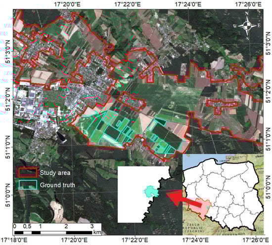
Figure 1.
Location of the study area.
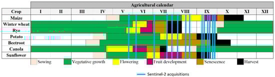
Figure 2.
Theoretical agricultural calendar for crop types cultivated in the study area overlaid with the period of Sentinel-1 acquisitions.
3.2. Data
Level 2A images from the Sentinel-2 mission with relative orbits 79 and 122 were used for classification. Weather conditions in the study area only allowed the collection of 14 cloud-free images at unequal time intervals, which are presented in Figure 2. In addition, it was necessary to capture field information about crop types in a specific region. For this purpose, 14 field visits were conducted between the dates of 18 May 2020 and 11 April 2020 to properly identify crop types.
Field inspection showed that in the study area there were seven crop types: beetroot, potato, canola, sunflower, maize, winter wheat, and rye. In total, 54 fields were identified, including 2 beetroot fields, 13 potato fields, 1 canola field, 4 sunflower fields, 17 maize fields, 15 winter wheat fields, and 2 rye fields. These data were used for training and testing the dataset.
3.3. Methodology
Figure 3 presents the flow chart applied in this study. After capturing 14 Sentinel-2 images, they were resampled at a B2 resolution of 10 m. Subsequently, for each Sentinel-2 image, 12 various spectral indices were calculated. Section 3.3.1. describes the computation of these indices in more detail. Many of these indices are correlated; therefore, principal component analysis (PCA) was utilized to remove redundancy of the data and to check whether the application of only first principal components without any data redundancy achieved the best results. Then, the detection of crop types based on random forest classification was carried out, as described in Section 3.3.3. Crop type classification was performed using the tools available in Esri ArcMap (version 10.8.1). This was performed separately for each index, for all indexes, for a group of selected indexes (MCARI, NDI4, and WDVI), and for different combinations of principal components (PCs). The accuracy of the classification was evaluated using various accuracy measures, as presented in Section 3.3.4.
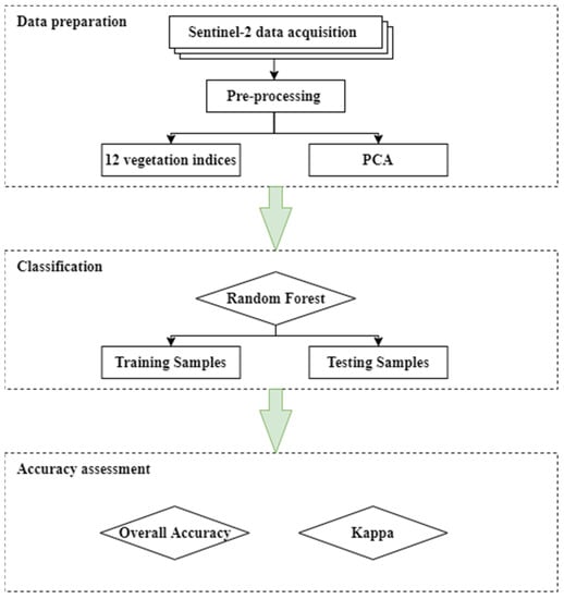
Figure 3.
Methodology workflow for crop type classification.
3.3.1. Vegetation Indices
The detection of crop species was performed based on 12 vegetation indices calculated from 14 Sentinel-2 images. Calculations were carried out in SNAP (version.8.0.2) and involved resampling in Band 2 (B2) with a 10 m resolution. Vegetation indices were calculated for multitemporal images between 30 May 2020 and 24 September 2020. PCA was carried out for all 12 spectral indices. Table 1 shows an overview of the used indices and a short description of each index used.

Table 1.
Spectral indices applied in the study. NIR—Near Infrared, R—Red band, G—Green bands and RE—Red Edge.
3.3.2. Principal Component Analysis
Principal component analysis (PCA) is one of the most popular multivariate statistical methods used in various fields of science; it allows to reduce the number of variables, while retaining the most important information from a dataset [41]. This method is based on finding linear combinations along which there is a maximum variability in the data, called principal components [42].
In order to apply PCA for spectral indices, it was necessary to assess their mutual correlation. The correlation matrix between these indices is shown in Table 2.
Table 2.
Correlation matrix of spectral indices for a Sentinel image captured on 05/30/20.
Based on the correlation matrix of the spectral indices, it can be stated that significant mutual correlations existed between the indices WDVI, SAVI, NDVI, NDI45, MSAVI, IRECI, and GNDVI. The correlation here was at a level of about 0.8–0.9. When analyzing the matrix, it can also be seen that the S2REP and REIP indices had a perfect correlation of 1 but showed almost no correlation with the rest of the coefficients. On this basis, it can be inferred that the application of additional correlated indices is not needed, because it contain redundant information.
PCA was performed for the 12 vegetation indices presented in Table 1. Figure 4 shows the accumulative eigenvalues for PCs. It can be seen that most of the information was contained in the first four components; therefore, we used these four PCs to evaluate the accuracy of crop type detection without making any information redundant.
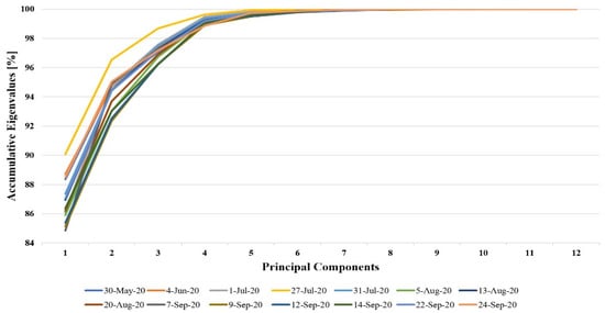
Figure 4.
Accumulative eigenvalues for the principal components.
3.3.3. Classification Using Random Forest
Random forest (RF) is a combinatorial ensemble learning classification algorithm [5]. It is designed to create multiple decision trees, which are trained on a bootstrapped sample of training data [43]. The algorithm can be described by the following equation [4]:
where h is the random forest classifier, x is an input variable, and {θk} is the independent identically distributed random predictor variables.
RF consists of many classifiers, which distinguishes it from traditional classification trees (CTs) and represents a new concept of classifiers [44]. The diversity of trees increases, because RF makes them grow from different subsets of training data through bootstrap aggregation and bagging [45]. In this method of classification, trees are used as base classifiers; thus, some data may be used more than once in classifier training, whereas others may never be used [44]. This makes the algorithm more robust to small changes in input data, increasing classification accuracy and making it more stable [44].
RF is widely used in remote sensing. It is known to run efficiently on large datasets with a large number of input variables, to estimate which variables are significant in the classification process, and is relatively robust to noise and outliers [44]. Numerous examples of the use of this algorithm can be found in the literature. Feng et al., (2019) [4] proposed a hybrid method using RF and texture analysis to accurately differentiate the land covers of urban vegetated areas and analyze changes in classification precision as a function of the texture window. An RF classifier consisting of 200 decision trees was used for classification in the spectral–textural feature space. Ground truth points were generated based on the information on crop types captured in the field.
Ground truth polygon data with agricultural fields were split into training and testing datasets. The training dataset consisted of 34.6% of all ground truths from the investigated field. The same training samples were used for each classification experiments. An RF classifier implemented within the European Space Agency open The Sentinel Application Platform SNAP (version 8.0.2) software was used for classification. A total of 5000 samples within the ground true data were used for training the model; 10% of the training samples were used for cross-validation for each classification to estimate model performance. Cross-validation indexes of all classification experiments carried out were at the level of 96–100%. Within RF classification in SNAP, only hyperparameters such as the number of training samples and number of trees can be modified and tuned by the user; other hyperparameters which are usually available for tuning in other software such as Python or R are not available in SNAP. However, in our approach, we performed a number of tests with different parameters and numbers of trees and training samples; in most cases, 100 trees and a 5000 training samples provided the best accuracy metrics. As accuracy metrics, the overall accuracy (OA) and Kappa coefficient were used. The accuracy metrics were calculated based on 500 ground truth points located in the area of testing.
3.3.4. Accuracy Measures
To verify the performance of crop type classification, it was necessary to perform an accuracy assessment. For this purpose, we computed the overall accuracy (OA) and the Kappa coefficient. OA is the total number of correctly classified samples (diagonals of the matrix). The precision of the whole image was measured without indicating the precision of individual categories [46]. OA can be described with the following equation:
Producer accuracy (PA) is the probability that a value in a given class was classified correctly. Having considered class number 1, PA is determined as follow:
User accuracy (UA) is the probability that a value predicted to be in a certain class really is that class. The probability is based on the fraction of correctly predicted values to the total number of values predicted to be in a class. Having considered positive class, PA is determined as follow
where:
- -
- true positive is an outcome where the model correctly predicts the positive class (TP).
- -
- true negative is an outcome where the model correctly predicts the negative class (TN).
- -
- false negative is an outcome where the model assigned observation to the negative class, which in reality belong to the positive class (FN),
- -
- false positive is an outcome where the model assign observation to positive class, which in reality belong to the negative class (FP),
- -
- N total number of pixels.
Kappa is a coefficient which was introduced by Cohen in 1960. In remote sensing, this is an index used to express the accuracy of the classification of an image [47]. In calculations of the Kappa coefficient, all elements of the error matrix are taken into consideration instead of just the diagonals of the matrix. The Kappa index provides a measure of how much better the classification performance is compared with the probability of randomly assigning pixels to their correct categories [48]. A kappa value of 1 represents perfect agreement, while a value of 0 represents no agreement [49]. The kappa coefficient is computed as follows:
where:
- i is the number of classes,
- N is the total number of classified values compared to truth values
- is the number of values belonging to the truth class i that have also been classified as class i (i.e., values found along the diagonal of the confusion matrix)
- is the total number of predicted values belonging to class i
- is the total number of truth values belonging to class i
4. Results
4.1. Effectiveness of Spectral Indices in Predicting Crop Type Detection
The main purpose of this study was to evaluate each vegetation index on the accuracy of crop type mapping. For the classification results, accuracy measures of OA and Kappa have been calculated and are presented in Figure 5 and Figure 6.
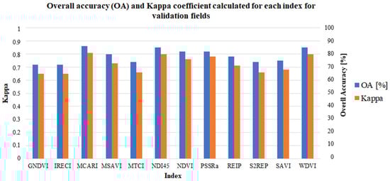
Figure 5.
OA and Kappa coefficient calculated for each index for the validation fields.
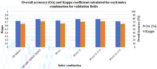
Figure 6.
Calculated OA and Kappa coefficient for each combination for the validation fields.
The highest values of OA and Kappa were obtained based on the MCARI (OA = 86%, Kappa = 0.81), NDI45 (OA = 85%, Kappa = 0.80), and WDVI (OA = 85%, Kappa = 0.80). On the other hand, both the GNDVI and IRECI exhibited the lowest accuracy (OA = 72% and Kappa = 0.65). Taking this into account, for the indices which demonstrated the best performance (MCARI, NDVI45, and WDVI) classification based on these three indices has been carried out. Unfortunately, despite the high accuracy of each of these indices used separately, their combination does not give better results (OA = 78%, Kappa = 0.72).
Furthermore, the results of the PCA showed that the highest accuracy could be obtained by using the initial two and three principal components. The accuracies of these variants were very close to each other, which may indicate that the three initial components contained most of the relevant information. However, these results do not have particularly high accuracy and may not be sufficient for the accurate detection of crop types. The use of only the first component provided an OA of 74% and Kappa of 0.66. The combination of the first four components provided an OA of 72% and Kappa of 0.65. Taking this into account, higher values have been delivered by MCARI or NDI45 or WDVI separately.
The classification performed by combining all the indices also did not generate more accurate results than the separate indexes alone (OA = 73% and Kappa = 0.65). This may be because each of the indices is slightly different and may respond differently to a given plant species. Although each of the indices used performed very well in detecting individual crop types, combining them could still lead to inconclusive results. Figure 7 shows a graphical representation of these results.
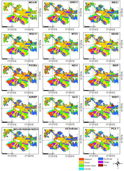
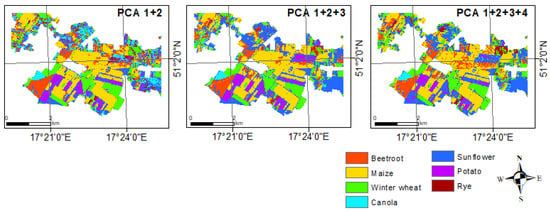
Figure 7.
Classification results for various experiments of crop type mapping.
4.2. Crop patterns in the Investigated Study Area
Based on the classification results derived from the MCARI, quantitative values of crop types within the study area were generated and are presented in Figure 8a. In contrast, Figure 8b presents the contribution of each crop type in the ground truth dataset. It is visible that similar contributions of different crop types are represented from ground truth as well as from classified results. This indicates that classification using MCARI enables the estimation of crop patterns in the analyzed areas at a larger scale. It could be observed that rye, sunflower, and canola were very rarely grown within the study area (1%, 5%, and 3%, respectively). The distributions of maize, winter wheat, and potato were quite similar, at a level of 24–30%, and were the crop types most widely cultivated in the study area.
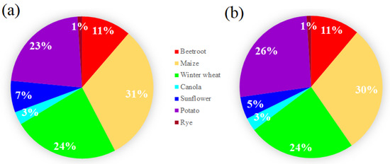
Figure 8.
Proportions of different crops grown in the investigated agricultural study areas based on MCARI classification (a) and for ground truth (b).
4.3. Feature Importance
Based on the feature importance provided by RF classification, it was possible to present the importance score (the first ten features ranked as the most important, as shown in Figure 9). Notably, in the classification using a single index, the index calculated on for 4 June 2020 usually appeared in first place. Then, 30 May 2020 and two images in August were the next most important. Having observed the scores, even then the acquisition date of 4 June 2020 did not appear in first place; this date was ranked in second place in another cases. This indicates that the images or the phenology period of June are most important for proper differentiation of the crop types. In the case of classification using all indices or by using PCA, no acquisition date repeats, which does not indicate any important phenology period for the proper crop type detection. However, classification results for these experiments were much lower than single-layer classification.
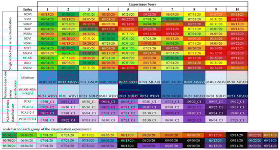
Figure 9.
Feature importance for each classification experiment. First part represents single index classification, second part represents multi index classification while third part represents PCA- based classification. Various color bars portrays specific acquisition dates in each of the classification experiments. Black color represent that this image is not within the top 10 important variables.
5. Discussion
Although all indices used in this study are closely related to the chlorophyll content of plants, their performance in crop field detection was found to vary slightly. This situation may be due to the different characteristics of each of these indices, the short time series used in this study, and the local settings. Surprisingly, the accuracy of the classification carried out for all investigated vegetation indices was not the highest as presented by other authors in literature (Zhang et al., (2020) [5], Utsuner et al., (2014) [17]). In some cases, crop type mapping based on each single vegetation index achieved higher accuracy than the integrated use of all indexes (MCARI, NDI45, and WDVI). Furthermore, Kobayshi et al., (2020) [16] also reported that the application of additional indices did not increase classification accuracy.
Figure 10 presents a graphical representation for the best and the worst results of the spectral-based classification and a comparison with the ground truth. As can be observed, mostly potato was classified as sunflower in the process with all indexes (the worst results). As can be seen, MCARI results corresponded relatively accurately with the ground truth. Both classification results provided noisy information in the northern part of the investigated area. This could have been caused by small agricultural fields in this area being problematic in correctly classifying the crop types.
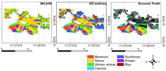
Figure 10.
Classification with the best and the worst spectral indices and comparison with the ground truth.
In Figure 11 and Figure 12, an NDVI and an MCARI time series is presented for the various crop types in the investigated study area, respectively. As can be observed, the time series of the NDVI was similar for maize and beetroot and for sunflower and potato, making them challenging to distinguish. This similar time series for these species is the answer for the false positives achieved in various classification tests as presented in Figure 8 and Figure 10. In addition to the similar NDVI time series responses of these species, the harvesting time of them is similar, which was also confirmed in Figure 2; the harvest (circles) and sowing periods of these two plants are comparable. This may present challenges in distinguishing between these two species. In contrast, another situation is presented by the MCARI. Maize and beetroot clearly have varying time series; this enables the more accurate detection of crop types. Unfortunately, we did not have access to cloud-free images in October; therefore, it was impossible to observe the spectral behavior of beetroot, maize, and sunflower.
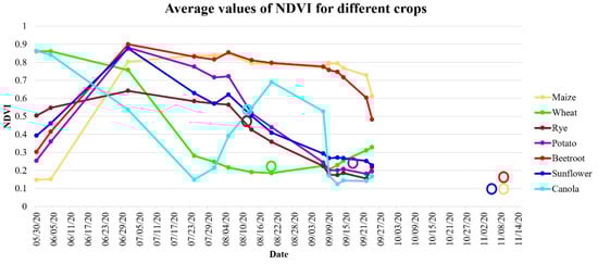
Figure 11.
Time series of the NDVI for different types of crops, calculated as average values of all fields with harvesting dates marked with circles.
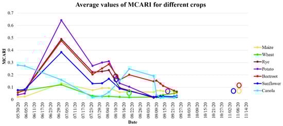
Figure 12.
Time series of the NDVI and MCARI for different types of crops, calculated as average values of all fields with harvesting dates marked with circles.
Another aspect worth investigating in the future is related to the investigated time period, which should be strictly adjusted to the phenological development of the plants. In this study, we captured images from May to September, which is not adequate to observe the development of all species. For example, wheat and canola were very well-developed plants in May, characterized by an NDVI value of 0.9. Therefore, to achieve better crop mapping results, it is worth covering the time period in which each of the plant species is sown and harvested. Therefore, a wider time series (preferably one year) would help differentiate between various crop species. Nevertheless, as presented in Figure 10, the period of June appears to be the most important in the detection of the plant species in our experiment. The reason for that is probably that the flowering, fruit development, and vegetation growth (Figure 2) appear for different plant species in that period. It is foreseen that the period of harvesting and sowing can also be the most important, since this is different for different plant species.
Based on the graphical representation of the classification results in Figure 10 and the PA and UA presented in Appendix A, it can be observed that in most cases the classification of corn and wheat fields is highly accurate. The reason for this may be the characteristics and unique late sowing time of corn in the study area. Sunflower, potato, and rye are characterized by a significantly lower detection accuracy. The reason for this may be the concentration of these plant fragments in the total investigated study area and unbalanced data. In 2020, the investigated research area was significantly dominated by cereal crops. When the samples were randomly generated and split into training and testing datasets, it may have turned out that most of these points came from beetroot, maize, and winter wheat; thus, the accuracy of the automatic detection of those species was higher. It is possible that these indexes could have shown greater efficiency in an area where more training samples could have been created for other plant species for a more balanced representation. Additionally, it is worth considering that the contribution of each crop type in the training samples will be similarly large.
Furthermore, when observing the classification results in Figure 11, we can see that a more accurate classification was presented in the area of training field location, whereas for the areas located further away from the training samples the classification results were noisier. This is mostly associated with the autocorrelation aspect introduced by the location of training within the training fields. This aspect should also be considered, because this procedure of splitting ground truths into training and testing data is more practical than a random sampling design (training fields/points evenly distributed across the whole study area). This is because it is easier to capture training samples during the field trips or farmers’ declarations in one concise study area rather than random and evenly distributed samples across the investigated study area (e.g., whole province or commune). This issue should also be taken into account when crop mapping is performed for large areas. For such analysis, it will be valuable to have training samples in various locations to properly describe remote sensing signals associated with various plant species. In this context, it is also worth considering that object-based image analysis (OBIA) does limit single false classification result or pixels located inside the field. Investigation of the field as a whole will be more advantageous.
Taking the classification accuracy measures into account, three indexes were the most satisfactory: MCARI, NDI45, and WDVI. These indices allowed for the accurate detection of fields not only of wheat and maize, but also of other cultivated plant species such as sunflower, potato, and beetroot (Appendix A). The difference between the behavior of these indexes and the others mentioned may concern their sensitivity to various crop species, the period of the multitemporal Sentinel-2A data, and local characteristics.
Classification performed on the basis of different combinations of PCA components has not provided higher accuracies. PCA was performed using the twelve vegetation indices; therefore, imperfections in the improper adjustment of the indices may have outweighed the advantages, resulting in lower accuracy in the detection of different plant species. Nevertheless, this indicates that the redundancy reduction based on 14 spectral indices applied in our case study do not increase classification accuracy. Additionally, when comparing the achieved results with some presented in the literature (Table 3), it can be concluded that in general the accuracy of automatic detection of cultivated plant species based on the Sentinel-2A multitemporal images was around the level of 85%. However, the application of other sensors such as Landsat may help to increase accuracy. However, as presented by Heupel et al., (2018) [14], this mostly depends on the weather conditions. Therefore, alternative methods are needed to integrate SAR and optical data for crop mapping.
Table 3.
Comparison of classification results in different studies.
6. Conclusions
The purpose of this study was to investigate the effectiveness of widely used vegetation indices calculated from Sentinel-2 images for the automatic detection of crop types using the random forest algorithm. The results showed that three vegetation indices yielded the highest accuracy, namely MCARI (OA = 86%, Kappa = 0.81), NDI45 (OA = 85%, Kappa = 0.81), and WDVI (OA = 85%, Kappa = 0.80). Although these indices have great potential when used separately, their combination led to lower accuracy (OA = 78%, Kappa = 0.72).
An additional goal of this study was to evaluate the effect of dimensionality reductions on automatic crop type mapping. However, four different combinations of components were used and the classification results and the reduction in the dimensionality using PCA did not show an increase in the mapping accuracy in all variants. For example, simultaneous use of the three initial PCA components exhibited an OA of 78% and Kappa coefficient of 0.72. Unfortunately, this is still not a satisfactory result.
Additionally, our experiments show that between April and September the most important period in which the spectral data should be captured is June and August. This is because in June, stages such as the flowering, fruit development, and vegetation growth (Figure 2) appear for different plant species in that period. Similarly, in September various species are harvested. Therefore, when designing the methodology for crop type detection, the images from key periods for each specific plant cultivated in the study should be included.
Vegetation indices show considerable potential for the automatic detection of crop fields. Using the MCARI, NDI45, and WDVI, we were able to accurately classify the fields in our selected study area. However, it should be taken into account that these indices may not show such satisfactory accuracy when classifying fields sown with crop species different from those presented in this study. In addition, a major drawback of optical data is the need to acquire cloudless images, which can be a very difficult task in some areas. In future research related to the automatic detection of fields, it will be worth considering additional optical images from other missions, as well as use of radar images which, because of their characteristics, can be acquired regardless of the time of day and weather conditions.
Author Contributions
Conceptualization, K.P.-F.; methodology, K.P.-F.; software, K.P.-F.; validation, K.P.-F.; formal analysis, K.P.-F. and M.P.; investigation, M.P.; resources, K.P.-F. and M.P.; data curation, M.P.; writing—original draft preparation, K.P.-F. and M.P.; writing—review and editing, K.P.-F. and M.P.; visualization, M.P.; supervision, K.P.-F.; project administration, K.P.-F.; funding acquisition, K.P.-F. and M.P. All authors have read and agreed to the published version of the manuscript.
Funding
This research was funded by the Ministry of Education and Science, grant number: MEiN/2021/205/DIR/NN4 under the program: “Best of the best! 4.0.”, under the Knowledge Education Development Operational Program co-financed by the European Social Fund (application number for funding, POWR.03.03.00-00-P019/18). The APC/BPC is financed/co-financed by Wroclaw University of Environmental and Life Sciences.
Data Availability Statement
Sentinel-2 data are freely available via https://scihub.copernicus.eu/ (accessed on 25 October 2020). Data containing information about the crop types in .shp captured within the field are available to share upon request.
Conflicts of Interest
The authors declare no conflict of interest.
Appendix A
Table A1.
User accuracy for the spectral indices used in this study.
Table A1.
User accuracy for the spectral indices used in this study.
| User Accuracy | ||||||||||||
|---|---|---|---|---|---|---|---|---|---|---|---|---|
| Class: | GNDVI | IRECI | MCARI | MSAVI | MTCI | NDI45 | NDVI | PSSRa | REIP | S2REP | SAVI | WDVI |
| Beetroot | 0.82 | 0.98 | 0.91 | 0.90 | 0.84 | 0.84 | 0.81 | 0.79 | 0.91 | 0.92 | 0.70 | 0.94 |
| Maize | 0.96 | 0.97 | 0.90 | 0.94 | 0.94 | 0.90 | 0.95 | 0.98 | 0.93 | 0.92 | 0.94 | 0.93 |
| Winter wheat | 0.99 | 0.98 | 0.98 | 0.98 | 0.94 | 0.98 | 0.99 | 0.99 | 0.94 | 0.91 | 0.99 | 0.99 |
| Canola | 0.94 | 0.94 | 1.00 | 1.00 | 0.84 | 1.00 | 0.94 | 1.00 | 0.67 | 0.76 | 0.89 | 1.00 |
| Sunflower | 0.23 | 0.23 | 0.61 | 0.33 | 0.27 | 0.54 | 0.40 | 0.25 | 0.32 | 0.31 | 0.37 | 0.43 |
| Potato | 0.88 | 0.89 | 0.87 | 0.87 | 0.86 | 0.87 | 0.87 | 0.90 | 0.88 | 0.87 | 0.87 | 0.89 |
| Rye | 0.43 | 0.57 | 0.57 | 0.57 | 0.43 | 0.60 | 0.57 | 0.57 | 0.50 | 0.30 | 0.57 | 0.50 |
Table A2.
Producer accuracy for the spectral indices used in this study.
Table A2.
Producer accuracy for the spectral indices used in this study.
| Producer Accuracy | ||||||||||||
|---|---|---|---|---|---|---|---|---|---|---|---|---|
| Class: | GNDVI | IRECI | MCARI | MSAVI | MTCI | NDI45 | NDVI | PSSRa | REIP | S2REP | SAVI | WDVI |
| Beetroot | 0.88 | 0.93 | 0.89 | 0.93 | 0.96 | 0.82 | 0.93 | 0.95 | 0.91 | 0.84 | 0.93 | 0.86 |
| Maize | 0.90 | 0.95 | 0.97 | 0.94 | 0.88 | 0.95 | 0.90 | 0.90 | 0.93 | 0.91 | 0.92 | 0.97 |
| Winter wheat | 0.94 | 0.94 | 0.93 | 0.93 | 0.91 | 0.93 | 0.93 | 0.94 | 0.91 | 0.91 | 0.94 | 0.92 |
| Canola | 1.00 | 1.00 | 1.00 | 1.00 | 1.00 | 1.00 | 1.00 | 1.00 | 1.00 | 1.00 | 1.00 | 1.00 |
| Sunflower | 0.70 | 0.81 | 0.63 | 0.70 | 0.74 | 0.70 | 0.70 | 0.74 | 0.74 | 0.67 | 0.70 | 0.70 |
| Potato | 0.58 | 0.45 | 0.86 | 0.71 | 0.54 | 0.82 | 0.80 | 0.56 | 0.62 | 0.63 | 0.64 | 0.82 |
| Rye | 0.30 | 0.40 | 0.40 | 0.40 | 0.30 | 0.30 | 0.40 | 0.40 | 0.20 | 0.30 | 0.40 | 0.40 |
Table A3.
User accuracy for combinations used in this study.
Table A3.
User accuracy for combinations used in this study.
| User Accuracy | ||||||
|---|---|---|---|---|---|---|
| Class: | MCARI + NDI45 + WDVI | All Indices | PCA1 | PCA1 + 2 | PCA1 + 2 + 3 | PCA1 + 2 + 3 + 4 |
| Beetroot | 0.71 | 0.89 | 0.83 | 0.96 | 0.94 | 0.89 |
| Maize | 0.95 | 0.96 | 0.93 | 0.93 | 0.95 | 0.97 |
| Winter wheat | 0.99 | 0.99 | 0.94 | 0.94 | 0.98 | 0.98 |
| Canola | 1.00 | 1.00 | 0.73 | 0.73 | 0.89 | 1.00 |
| Sunflower | 0.41 | 0.25 | 0.27 | 0.30 | 0.29 | 0.24 |
| Potato | 0.86 | 0.87 | 0.86 | 0.88 | 0.91 | 0.89 |
| Rye | 0.44 | 0.31 | 0.60 | 0.60 | 0.43 | 0.40 |
Table A4.
Producer accuracy for combinations used in this study.
Table A4.
Producer accuracy for combinations used in this study.
| Producer Accuracy | ||||||
|---|---|---|---|---|---|---|
| Class: | MCARI + NDI45 + WDVI | All Indices | PCA1 | PCA1 + 2 | PCA1 + 2 + 3 | PCA1 + 2 + 3 + 4 |
| Beetroot | 0.91 | 0.91 | 0.86 | 0.93 | 0.89 | 0.91 |
| Maize | 0.95 | 0.95 | 0.90 | 0.93 | 0.92 | 0.94 |
| Winter wheat | 0.95 | 0.91 | 0.90 | 0.93 | 0.93 | 0.91 |
| Canola | 1.00 | 1.00 | 1.00 | 1.00 | 1.00 | 1.00 |
| Sunflower | 0.70 | 0.74 | 0.63 | 0.67 | 0.74 | 0.78 |
| Potato | 0.64 | 0.53 | 0.63 | 0.65 | 0.71 | 0.50 |
| Rye | 0.40 | 0.40 | 0.30 | 0.30 | 0.30 | 0.40 |
References
- Jaworek, D.; Podsiadło, M.; Wankat, A. Agencja Restrukturyzacji i Modernizacji Rolnictwa; Uniwersytet Śląski w Katowicach: Katowice, Poland, 2013. (In Polish) [Google Scholar]
- Sun, C.; Bian, Y.; Zhou, T.; Pan, J. Using of multi-source and multi-temporal remote sensing data improves crop-type mapping in the subtropical agriculture region. Sensors 2019, 19, 2401. [Google Scholar] [CrossRef] [PubMed] [Green Version]
- Vuolo, F.; Neuwirth, M.; Immitzer, M.; Atzberger, C.; Ng, W.T. How much does multi-temporal Sentinel-2 data improve crop type classification? Int. J. Appl. Earth Obs. Geoinf. 2018, 72, 122–130. [Google Scholar] [CrossRef]
- Feng, S.; Zhao, J.; Liu, T.; Zhang, H.; Zhang, Z.; Guo, X. Crop type identification and mapping using machine learning algorithms and sentinel-2 time series data. IEEE J. Sel. Top. Appl. Earth Obs. Remote Sens. 2019, 12, 3295–3306. [Google Scholar] [CrossRef]
- Zhang, H.; Kang, J.; Xu, X.; Zhang, L. Accessing the temporal and spectral features in crop type mapping using multi-temporal Sentinel-2 imagery: A case study of Yi’an County, Heilongjiang province, China. Comput. Electron. Agric. 2020, 176, 105618. [Google Scholar] [CrossRef]
- Busquier, M.; Lopez-Sanchez, J.M.; Mestre-Quereda, A.; Navarro, E.; González-Dugo, M.P.; Mateos, L. Exploring TanDEM-X interferometric products for crop-type mapping. Remote Sens. 2020, 12, 1774. [Google Scholar] [CrossRef]
- Mestre-Quereda, A.; Lopez-Sanchez, J.M.; Vicente-Guijalba, F.; Jacob, A.W.; Engdahl, M.E. Time-series of Sentinel-1 interferometric coherence and backscatter for crop-type mapping. IEEE J. Sel. Top. Appl. Earth Obs. Remote Sens. 2020, 13, 4070–4084. [Google Scholar] [CrossRef]
- Wu, M.; Yang, C.; Song, X.; Hoffmann, W.C.; Huang, W.; Niu, Z.; Wang, C.; Li, W. Evaluation of orthomosics and digital surface models derived from aerial imagery for crop type mapping. Remote Sens. 2017, 9, 239. [Google Scholar] [CrossRef] [Green Version]
- Nowakowski, A.; Mrziglod, J.; Spiller, D.; Bonifacio, R.; Ferrari, I.; Mathieu, P.P.; Garcia-Herranz, M.; Kim, D.H. Crop type mapping by using transfer learning. Int. J. Appl. Earth Obs. Geoinf. 2021, 98, 102313. [Google Scholar] [CrossRef]
- Torbick, N.; Huang, X.; Ziniti, B.; Johnson, D.; Masek, J.; Reba, M. Fusion of moderate resolution earth observations for operational crop type mapping. Remote Sens. 2018, 10, 1058. [Google Scholar] [CrossRef] [Green Version]
- Adrian, J.; Sagan, V.; Maimaitijiang, M. Sentinel SAR-optical fusion for crop type mapping using deep learning and Google Earth Engine. ISPRS J. Photogramm. Remote Sens. 2021, 175, 215–235. [Google Scholar] [CrossRef]
- Yan, Y.; Ryu, Y. Exploring Google Street View with deep learning for crop type mapping. ISPRS J. Photogramm. Remote Sens. 2021, 171, 278–296. [Google Scholar] [CrossRef]
- Zhao, H.; Duan, S.; Liu, J.; Sun, L.; Reymondin, L. Evaluation of Five Deep Learning Models for Crop Type Mapping Using Sentinel-2 Time Series Images with Missing Information. Remote Sens. 2021, 13, 2790. [Google Scholar] [CrossRef]
- Heupel, K.; Spengler, D.; Itzerott, S. A progressive crop-type classification using multitemporal remote sensing data and phenological information. PFG–J. Photogramm. Remote Sens. Geoinf. Sci. 2018, 86, 53–69. [Google Scholar] [CrossRef] [Green Version]
- Gumma, M.K.; Tummala, K.; Dixit, S.; Collivignarelli, F.; Holecz, F.; Kolli, R.N.; Whitbread, A.M. Crop type identification and spatial mapping using Sentinel-2 satellite data with focus on field-level information. Geocarto Int. 2020, 1–17. [Google Scholar] [CrossRef]
- Kobayashi, N.; Tani, H.; Wang, X.; Sonobe, R. Crop classification using spectral indices derived from Sentinel-2A imagery. J. Inf. Telecommun. 2020, 4, 67–90. [Google Scholar] [CrossRef]
- Ustuner, M.; Sanli, F.B.; Abdikan, S.; Esetlili, M.T.; Kurucu, Y. Crop type classification using vegetation indices of rapideye imagery. Int. Arch. Photogramm. Remote Sens. Spat. Inf. Sci. 2014, 40, 195. [Google Scholar] [CrossRef] [Green Version]
- Zhong, L.; Hu, L.; Zhou, H. Deep learning based multi-temporal crop classification. Remote Sens. Environ. 2019, 221, 430–443. [Google Scholar] [CrossRef]
- Kussul, N.; Lavreniuk, M.; Skakun, S.; Shelestov, A. Deep learning classification of land cover and crop types using remote sensing data. IEEE Geosci. Remote Sens. Lett. 2017, 14, 778–782. [Google Scholar] [CrossRef]
- Zheng, Y.Y.; Kong, J.L.; Jin, X.B.; Wang, X.Y.; Su, T.L.; Zuo, M. CropDeep: The crop vision dataset for deep-learning-based classification and detection in precision agriculture. Sensors 2019, 19, 1058. [Google Scholar] [CrossRef] [Green Version]
- Stromann, O.; Nascetti, A.; Yousif, O.; Ban, Y. Dimensionality reduction and feature selection for object-based land cover classification based on Sentinel-1 and Sentinel-2 time series using Google Earth Engine. Remote Sens. 2019, 12, 76. [Google Scholar] [CrossRef] [Green Version]
- Gao, J.; Nuyttens, D.; Lootens, P.; He, Y.; Pieters, J.G. Recognising weeds in a maize crop using a random forest machine-learning algorithm and near-infrared snapshot mosaic hyperspectral imagery. Biosyst. Eng. 2018, 170, 39–50. [Google Scholar] [CrossRef]
- Liu, Z.; Li, C.; Wang, Y.; Huang, W.; Ding, X.; Zhou, B.; Wu, H.; Wang, D.; Shi, J. Comparison of Spectral Indices and Principal Component Analysis for Differentiating Lodged Rice Crop from Normal Ones. IFIP Adv. Inf. Commun. Technol. 2012, 369, 84–92. [Google Scholar] [CrossRef] [Green Version]
- Gilbertson, J.K.; van Niekerk, A. Value of dimensionality reduction for crop differentiation with multi-temporal imagery and machine learning. Comput. Electron. Agric. 2017, 142, 50–58. [Google Scholar] [CrossRef]
- Jiang, Y.; Lu, Z.; Li, S.; Lei, Y.; Chu, Q.; Yin, X.; Chen, F. Large-scale and high-resolution crop mapping in china using sentinel-2 satellite imagery. Agriculture 2020, 10, 433. [Google Scholar] [CrossRef]
- Kabala, C.; Bekier, J.; Bińczycki, T.; Bogacz, A.; Bojko, O.; Cuske, M.; Woźniczka, P. Soils of Lower Silesia: Origins, Diversity and Protection; PTG, PTSH: Wrocław, Poland, 2015; 256p. [Google Scholar]
- Główny Inspektorat Ochrony Środowiska, Województwo Dolnośląskie. Available online: http://www.gios.gov.pl/images/dokumenty/pms/raporty/DOLNOSLASKIE.pdf (accessed on 18 December 2021). (In Polish)
- Kochanowska, J.; Dziedzic, M.; Gruszecki, J.; Lis, J.; Pasieczna, A.; Wołkowicz, S. Objaśnienia Do Mapy Geośrodowiskowej Polski 1: 50,000, Arkusz Laskowice (765); PIG: Warszawa, Poland, 2004. (In Polish) [Google Scholar]
- Wróblewski, K.; Pasternak, A. Przewodnik po Ziemi Jelczańsko-Laskowickiej; Local Newspeper in Polish; Urząd Miasta i Gminy w Jelczu-Laskowicach: Jelcz-Laskowice, Poland, 2005. [Google Scholar]
- Gitelson, A.A.; Kaufman, Y.J.; Merzlyak, M.N. Use of a green channel in remote sensing of global vegetation from EOS-MODIS. Remote Sens. Environ. 1996, 58, 289–298. [Google Scholar] [CrossRef]
- Frampton, W.J.; Dash, J.; Watmough, G.; Milton, E.J. Evaluating the capabilities of Sentinel-2 for quantitative estimation of biophysical variables in vegetation. ISPRS J. Photogramm. Remote Sens. 2013, 82, 83–92. [Google Scholar] [CrossRef] [Green Version]
- Daughtry, C.S.; Walthall, C.L.; Kim, M.S.; De Colstoun, E.B.; McMurtrey Iii, J.E. Estimating corn leaf chlorophyll concentration from leaf and canopy reflectance. Remote Sens. Environ. 2000, 74, 229–239. [Google Scholar] [CrossRef]
- Qi, J.; Chehbouni, A.; Huete, A.R.; Kerr, Y.H.; Sorooshian, S. A modified soil adjusted vegetation index. Remote Sens. Environ. 1994, 48, 119–126. [Google Scholar] [CrossRef]
- Dash, J.; Curran, P.J. The MERIS terrestrial chlorophyll index. Int. J. Remote Sens. 2004, 25, 5403–5413. [Google Scholar] [CrossRef]
- Delegido, J.; Verrelst, J.; Alonso, L.; Moreno, J. Evaluation of sentinel-2 red-edge bands for empirical estimation of green LAI and chlorophyll content. Sensors 2011, 11, 7063–7081. [Google Scholar] [CrossRef] [Green Version]
- Rouse, J.W.; Haas, R.H.; Schell, J.A.; Deering, D.W.; Freden, S.C.; Mercanti, E.P.; Becker, M.A. Monitoring vegetation systems in the great plains with ERTS. In Proceedings of the the Third ERTS Symposium, Washington DC, USA, 10–14 December 1973; Volume I, pp. 309–317. Available online: https://ntrs.nasa.gov/api/citations/19740022614/downloads/19740022614.pdf (accessed on 5 May 2022).
- Blackburn, G.A. Spectral indices for estimating photosynthetic concentrations: A test using senescent tree leaves. Int. J. Remote Sens. 1998, 19, 657–675. [Google Scholar] [CrossRef]
- Darvishzadeh, R.; Atzberger, C.; Skidmore, A.K.; Abkar, A.A. Leaf Area Index derivation from hyperspectral vegetation indicesand the red edge position. Int. J. Remote Sens. 2009, 30, 6199–6218. [Google Scholar] [CrossRef]
- Huete, A.R. A soil-adjusted vegetation index (SAVI). Remote Sens. Environ. 1988, 25, 295–309. [Google Scholar] [CrossRef]
- Clevers, J.G.P.W. The derivation of a simplified reflectance model for the estimation of leaf area index. Remote Sens. Environ. 1988, 25, 53–70. [Google Scholar] [CrossRef]
- Jolliffe, I. Principal component analysis. In Encyclopedia of Statistics in Behavioral Science; John Wiley&Sons, Ltd.: Hoboken, NJ, USA, 2005. [Google Scholar]
- Ringnér, M. What is principal component analysis? Nat. Biotechnol. 2008, 26, 303–304. [Google Scholar] [CrossRef]
- Gislason, P.O.; Benediktsson, J.A.; Sveinsson, J.R. Random forest classification of multisource remote sensing and geographic data. In Proceedings of the IGARSS 2004, 2004 IEEE International Geoscience and Remote Sensing Symposium, Anchorage, AK, USA, 20–24 September 2004; IEEE: Piscataway, NJ, USA, 2004; Volume 2, pp. 1049–1052. [Google Scholar]
- Rodriguez-Galiano, V.F.; Ghimire, B.; Rogan, J.; Chica-Olmo, M.; Rigol-Sanchez, J.P. An assessment of the effectiveness of a random forest classifier for land-cover classification. ISPRS J. Photogramm. Remote Sens. 2012, 67, 93–104. [Google Scholar] [CrossRef]
- Breiman, L. Bagging predictors. Mach. Learn. 1996, 24, 123–140. [Google Scholar] [CrossRef] [Green Version]
- Story, M.; Congalton, R.G. Accuracy assessment: A user’s perspective. Photogramm. Eng. Remote Sens. 1986, 52, 397–399. [Google Scholar]
- Foody, G.M. Explaining the unsuitability of the kappa coefficient in the assessment and comparison of the accuracy of thematic maps obtained by image classification. Remote Sens. Environ. 2020, 239, 111630. [Google Scholar] [CrossRef]
- Senseman, G.M.; Bagley, C.F.; Tweddale, S.A. Accuracy Assessment of the Discrete Classification of Remotely-Sensed Digital Data for Landcover Mapping; Construction Engineering Research Lab (Army): Champaign, IL, USA, 1995. [Google Scholar]
- Stehman, S. Estimating the kappa coefficient and its variance under stratified random sampling. Photogramm. Eng. Remote Sens. 1996, 62, 401–407. [Google Scholar]
Publisher’s Note: MDPI stays neutral with regard to jurisdictional claims in published maps and institutional affiliations. |
© 2022 by the authors. Licensee MDPI, Basel, Switzerland. This article is an open access article distributed under the terms and conditions of the Creative Commons Attribution (CC BY) license (https://creativecommons.org/licenses/by/4.0/).