1. Introduction
In recent years, degenerate polymerase chain reaction (PCR) technology has been widely used in new gene cloning, gene expression detection, virus detection and genome research. It has the advantages of rapidity, simplicity, and high sensitivity [
1]. A PCR primer sequence is called degenerate if some of its positions have several possible bases. The degeneracy of the primer is the number of unique sequence combinations it contains. This can improve the coverage of DNA template, but values that are too high will reduce the specificity of PCR. Therefore, the suitability of degenerate primers directly affects the success rate of PCR.
The design of degenerate primers can be described as a given set of n strings and integers k, d and m, looking for a primer of length k and degeneracy of at most d that matches at least m input strings [
2,
3].
In traditional primer design, if primers are required to match the target DNA sequence and some unknown sequences as much as possible, the number of bases at each position along the sequence is typically counted, and the appropriate primer length to minimize its length determined [
4]. However, this method is often used, due to the inconsistency between the sequence and inappropriate fitness evaluation function, during operations in primers with higher degeneracy. Therefore, in the process of primer design, primers should usually be selected to match some but not all of the target DNA sequence.
In recent years, iterative heuristic algorithms have been widely used to solve primer design problems. Treeratanajaru W et al. [
5] proposed a method using dynamic pattern matching to complete the design of degenerate primers, inputting nucleotide sequences from different bacteria into a system consisting of three steps: data reconstruction, primer design and attribute filtering, freely combining the results with Gibbs, and designing and selecting the most suitable sequence as a series of primers. Balla S et al. [
6] proposed an algorithm for designing the minimum degeneracy of degenerate primers for a given DNA sequence that combined the topic discovery methodology and iterative technology to perform testing and comparison in random and real biological data sets. Souvenir R et al. [
7] proposed an iterative beam search algorithm and multiple iterative primer selector for the design of multiple degenerate primers that was superior to existing related algorithms for degenerate primer design and had a smaller number of stray amplifiers. Wu J S et al. [
8] proposed the use of the genetic algorithm to solve the primer design problem, and the constraint conditions of primer design were described using symbols and formulations; the algorithm was able to design primers meeting the requirements of specific restriction sites and specificity. Liang H L et al. [
9] proposed a new method for designing multiple PCR primers using the genetic algorithm and the MAP model; this method found several sets of appropriate primer pairs for five gene family cDNA templates, which were not only able to meet many primer design constraints, but also made the primers specific. In addition, software systems based on iterative heuristic algorithms have been developed for the design of degenerate primers, such as Primer 3 [
10], Primo Degenerate 3.4 [
11], CODEHOP [
12], etc. Linhart C et al. [
13] introduced the design of maximum coverage degenerate primers and minimum degeneracy primers, and developed a program named HYDEN on the basis of the proposed approximate algorithm, successfully applying it for the identification of olfactory receptor genes in mammals. Cickovski T et al. [
14] used existing algorithms to design cluster-based degenerate primers, and applied them in parallel in the GPUDePiCt software package using the shared memory model and graphics processing units (GPUs) to accelerate processing, and tested them in a large number of sequences in the human genome.
As can be seen from the above studies on degenerate primers, there are three cases addressed by research on degenerate primer design: maximum coverage degenerate primer design, that is, given a set of n strings, find a primer with length k to match as many strings as possible; minimum degeneracy degenerate primer design, that is, given a positive integer d, m and a set with n strings, find a primer with length k, make it match at least m strings and have the minimum degeneracy d; and design of minimum degeneracy primers that allow mismatches, that is, given positive integers d, e and a set with n strings, find a primer of length k that matches at least m strings, has minimum degeneracy d, and allows at most e mismatches. A finite number of mispairing experiments have little effect on the results and can also improve the amplification efficiency of primers.
Most of the existing methods are suitable for one or two cases of degenerate primer design, but it is difficult to solve more complex problems.
In addition, the swarm intelligence optimization algorithms [
15,
16] emerging in recent years have been demonstrated to be an effective means of solving complex optimization problems. Among them, the artificial bee colony algorithm offers good performance. Its application for solving practical problems in various fields has been attracting attention [
17,
18,
19,
20]. Therefore, this paper studies a solution method for degenerate primer design based on the artificial bee colony algorithm.
The main contributions of this paper are as follows: (1) A method based on the artificial bee colony algorithm for solving degenerate primer design problems is proposed that can not only meet the constraints of primer design, but also allows mismatch while considering the coverage and degeneracy of primers. (2) Combining the optimization process of the artificial bee colony algorithm and the ant colony algorithm, an optimization model of the hybrid artificial bee colony algorithm is constructed. (3) Based on the idea of the ant colony algorithm, the foraging strategies of all kinds of bees are redesigned, and a search space model and pheromone matrix are constructed.
2. Problem Description
The aim of this paper is to find the degenerate primer with the minimum degeneracy and the maximum coverage among all possible candidate primers in the case of a small number of base mismatches. To facilitate evaluation, for any candidate primer
P, the coverage and degeneracy were evaluated in this paper using Formula (1).
In Formula (1), Unconverge() represents the uncovering function, that is, the number of primers that failed to match DNA template sequences. For example, if there are 10 groups of target DNA sequences and a candidate primer P completes matching with 6 groups of target sequences, the uncoverage is 4. Degeneracy() stands for a degeneracy function whose degeneracy is at most d. Degeneracy refers to a degenerate PCR primer as a primer sequence that contains several possible bases in one or more positions. For example, both DNA and primer sequences are composed of four bases of AGCT. Assuming that there is a primer P, P = {A}{AC}{GT}{ATG}, then the length k of P is 4 and the degeneracy d = 1 × 2 × 2 × 3 is 12. μ and φ are the corresponding weight parameters.
In addition, for a pair of candidate primers, the following constraints need to be met in this study:
In general, the primer length should be between 18 and 26 bps. The
length() function is defined to represent the length of the primer, and its length is the sum of the number of bases at each position, as shown in Formula (2).
where |
P| indicates the total number of bases in primer
P.
The differential length of a primer pair is restricted to being smaller than 3 bps.
Pforward denotes the forward primers in a primer pair, and
Preverse denotes the reverse primers in a primer pair. Define
lengd() function to represent the length difference of primer pairs, as shown in Formula (3).
In general, the primer design has strict requirements on temperature. An empirical formula was proposed by Wallace for calculating the melting temperature of a primer
P with a length between 18 and 26 bps. This function
Tm() can be written as in Formula (4).
This simple formula depends directly on the length and composition of the primer. #
G indicates the amount of nucleotide “
A” in
P, #
T indicates the amount of nucleotide “
T” in
P; #
C and #
G can then be defined accordingly. Additionally, the differential melting temperature of a primer pair must be under 2 °C. The
Tmd() function is as shown in Formula (5).
The
GC content is the ratio of the number of nucleotide “
G”s and the number of nucleotide “
C”s in the primer
P sequence. It should be limited to within a certain range. In general, an appropriate range of
GC content for a primer is between 40% and 60%. The
GC content
GC(
P) is as shown in Formula (6).
where #
G indicates the number of nucleotide “
G”s in
P, and #C indicates the number of nucleotide “
C”s in
P. The
GCcontent(
P) function is as shown in Formula (7).
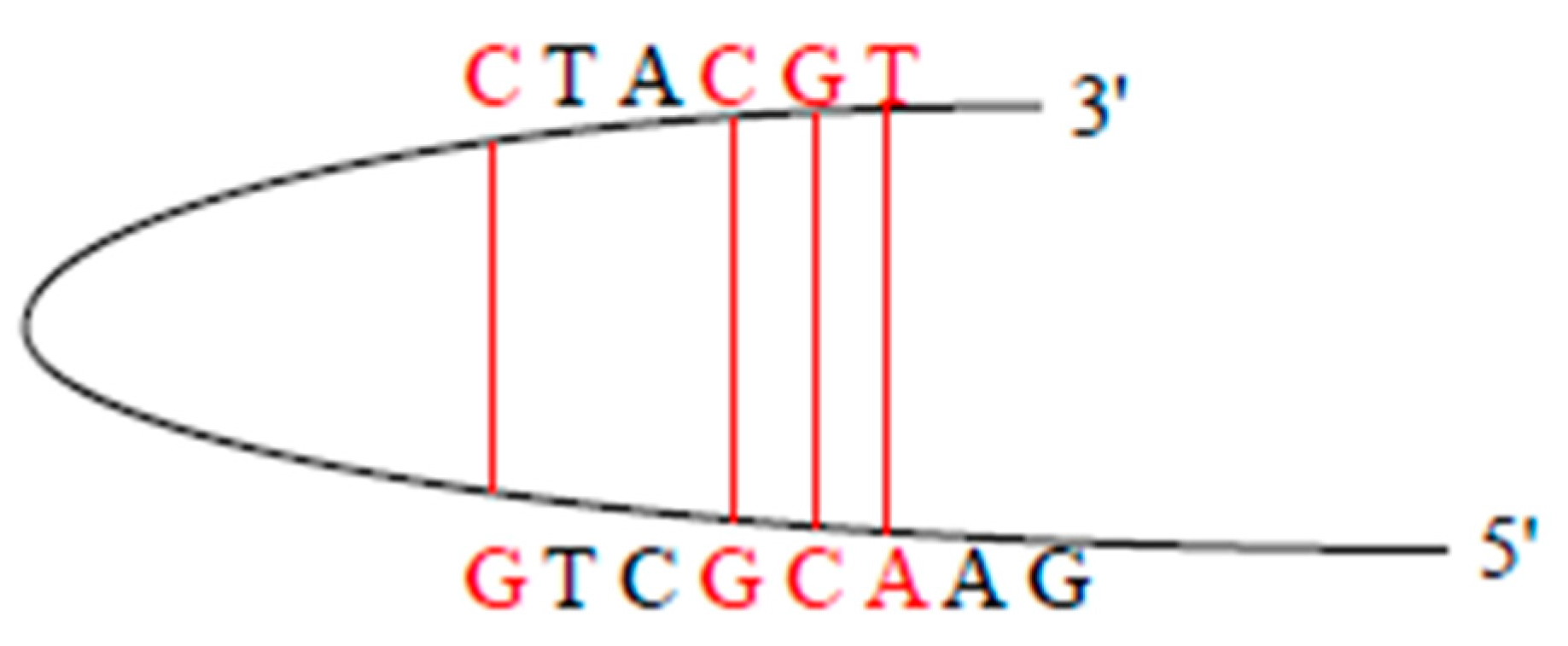
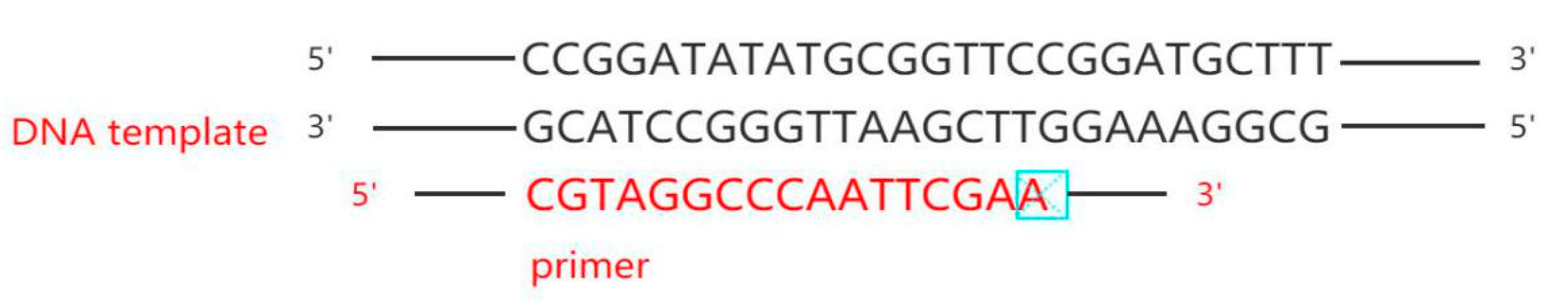
The 3′ end of a primer cannot choose nucleotide “
A”, it is better to choose nucleotide “
T”. When the 3′ end of a primer is mismatched, the last position is nucleotide “
A”, the chain synthesis can be triggered even under mismatched conditions. However, when the last position is nucleotide “
T”, mismatch initiation efficiency will be greatly reduced. The initiation efficiency of the nucleotide “
G” and nucleotide “
C” mismatch is between nucleotide “
A” and nucleotide “
T”, so nucleotide “
T” is the best choice for the 3′ end. See
Figure 1.
The
isGorC() function is used to represent the 3′ end of the primer
P with the nucleotides “
G”, “
C”, “
GC” and “
CG”, which is as shown in Formula (8).
Primers themselves should not have complementary sequences (no consecutive 4 bp complementarities), otherwise the primers themselves will fold into hairpin structures (as shown in
Figure 2), thus affecting the combination of the primer and the template.
The
Sc() function is used to indicate whether the primers themselves form a hairpin structure, as shown in Formula (9).
There should also be no complementary sequences between the primer chains. In other words, there should be no complementarity between the forward primer and the reverse primer, and there should not be four consecutive bases of complementarity between the primer chains; in particular, the complementary overlap of the 3′ end should be avoided in order to prevent the formation of a primer double chain (or dimer). The
Pc() function was used to indicate whether double chain structures were formed between primer chains, as shown in Formula (10).
3. The Proposed Algorithm
The aim of the proposed algorithm is to design degenerate primers. The degenerate primer design–hybrid artificial bee colony algorithm (DPD-HABC) is designed according to the construction process of candidate solutions and the use of pheromones.
The proposed algorithm mainly includes the representation of search space, updating of the pheromone matrix and the design of the foraging strategy. The model used to represent the search space defines the search space of the bee colony for the degenerate primer design problem and provides a representation of the food source. Since all kinds of bees share and exchange information through various pheromones in the process of foraging, the pheromone matrix and its update mode should be described first in the foraging process, before describing the foraging strategy. The representation of the search space, the updating of the pheromone matrix, and the design of the foraging strategy in this algorithm will be introduced in detail below.
3.1. Representation of the Search Space
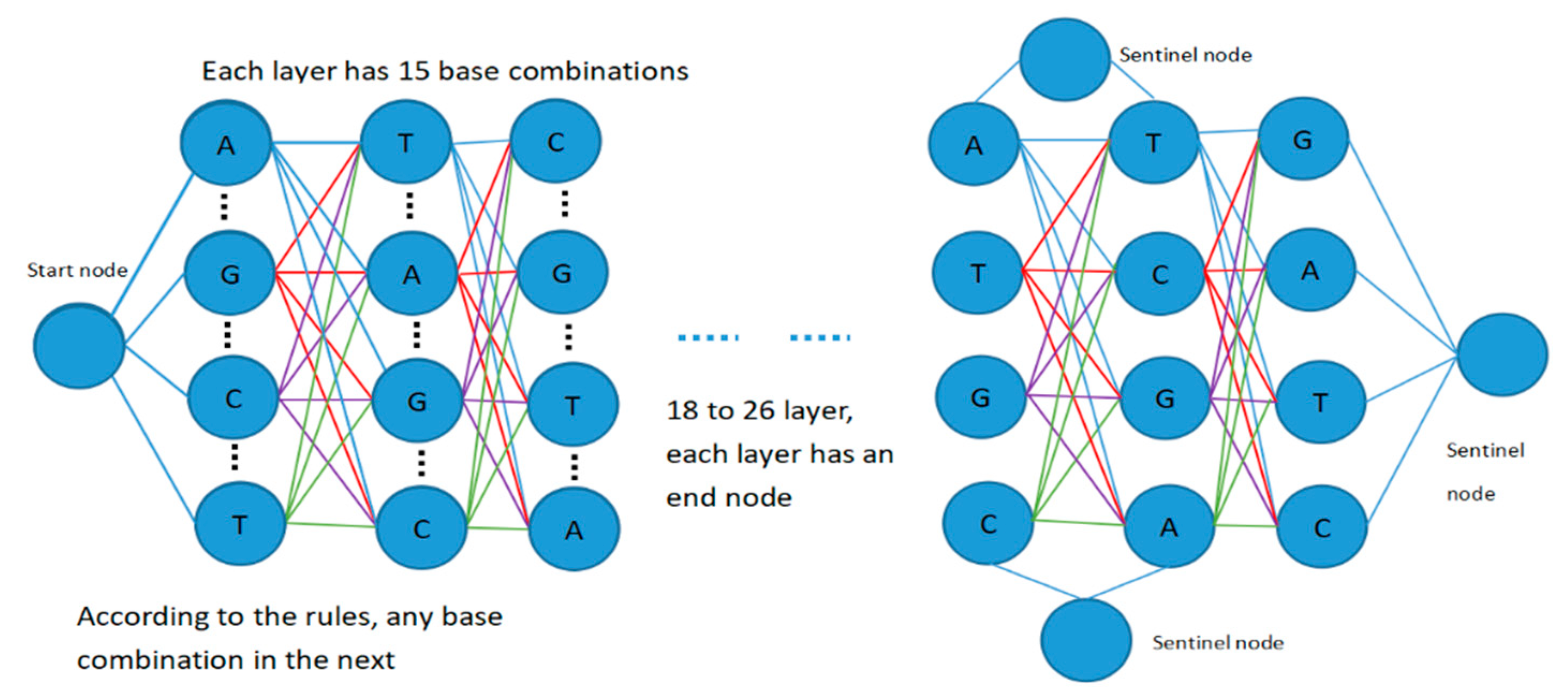
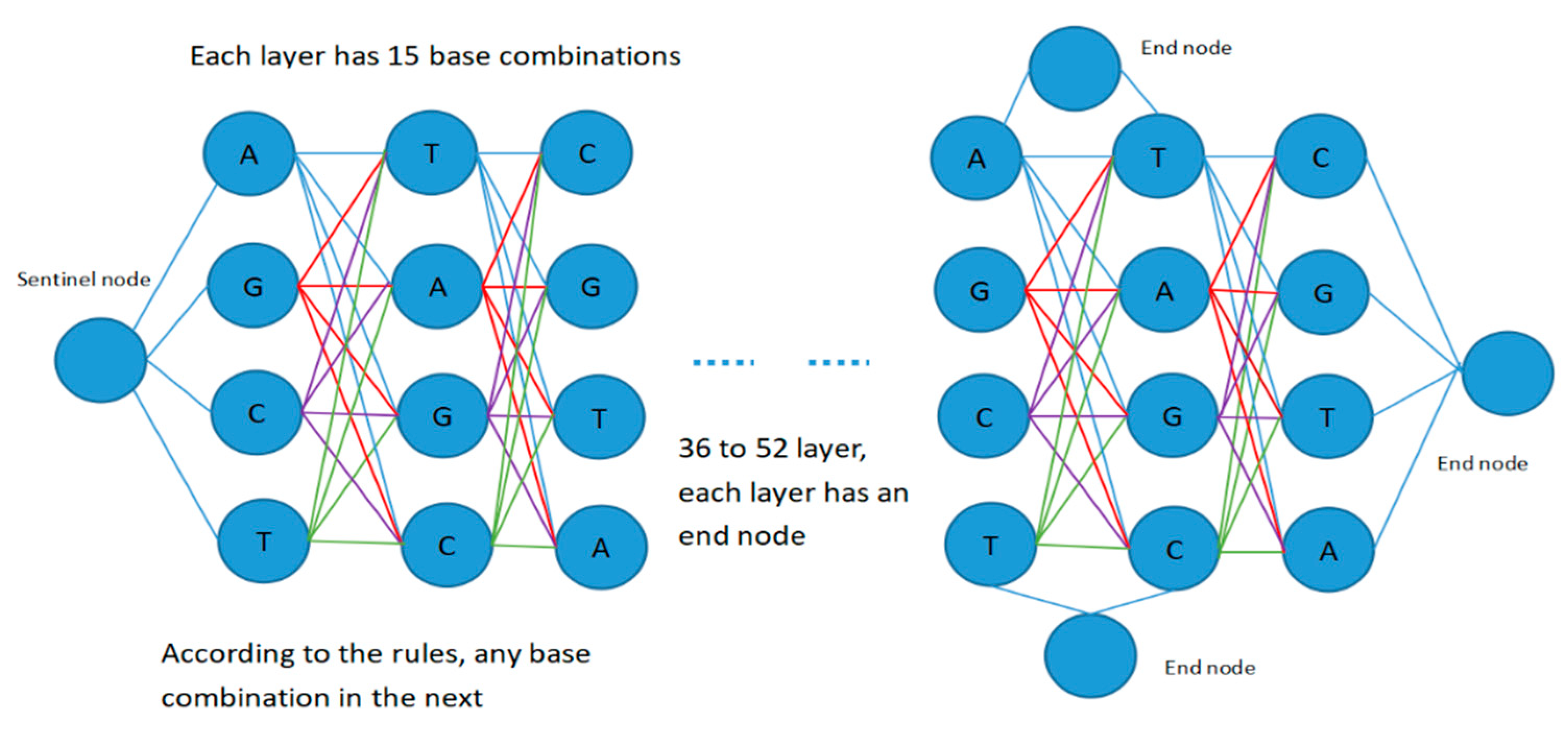
For the degenerate primer design problem, each candidate solution is a primer pair, including a forward candidate primer and a reverse candidate primer, and the lengths of the forward primer and the reverse primer are between 18 and 26. Therefore, the search space for degenerate primer design can be expressed as a fully connected graph structure with 55 layers, as shown in
Figure 3.
The diagram contains four types of node: start node, intermediate node, sentinel node, and end node. The middle nodes of each layer are successively set as an effective combination of four base pairs, such as nucleotide “A”, “T”, “C”, “G”, “AT”, “AC”, “AG”, “TC”, “TG”, “CG”, “ATC”, “ATG”, “TCG”, “ACG”, “ATCG”, etc. Sentinel nodes are mainly used to separate the forward primer and reverse primer, representing the end of the forward primer and the beginning of the reverse primer.
Setting up multiple sentinel nodes and end nodes is mainly performed to deal with the problem caused by variable primer length and to facilitate the completion of forward and reverse primer design. In each layer, appropriate base combination branches are selected according to the rules of base pairing and the constraints of coverage and degeneracy, and the cycle is iterated until appropriate primer pairs have been searched for and output results have been obtained or the maximum number of iterations has been reached. Then, the output results are filtered on the basis of primer design constraints, and the primer pairs and parameters of the forward and reverse primers that meet the requirements of the constraints are finally output.
In the process of constructing the search space, each bee constructs a candidate food source from the starting node in
Figure 3, and calculates the selection probability of the next optional node in accordance with the probability state transition formula adopted by the next optional node according to its category (i.e., employed bee, onlooker bee, or scout bee). The next node to visit is then selected by means of a roulette game. For each bee, including the intermediate nodes in the next layer, several bases or base combinations that meet the requirements are screened on the basis of the input template DNA sequence and the base matching principle, and then the selection probability of the corresponding nodes is calculated. In this way, nodes are selected layer by layer until an end node is encountered. Therefore, in addition to the above 15 base combinations, an end node is also set at nodes 46 to 54, so that the construction of the candidate food sources can be completed at any time. In this way, each bee completes the construction process of a candidate food that completes the design of a candidate primer pair.
3.2. Update of the Pheromone Matrix
In order to construct candidate food sources with variable lengths, the pheromone concept employed in ant colony optimization is used in the artificial bee colony algorithm. The DPD-HABC algorithm contains two kinds of pheromone matrix: the global pheromone matrix and the local pheromone matrix.
The global pheromone matrix mainly identifies the preferred search area of the current employed bee group and represents information on the current group’s search experience. Each employed bee sets up a local information matrix to record the individual search experience information it has obtained so far. In this way, each bee is able to forage according to the current search experience information of the whole population or the search experience information of individual employed bees. In the process of constructing candidate food sources, the greater the number of pheromones on a given side of the search space, the greater the probability of that side being selected.
In the DPD-HABC algorithm, when all employed bees have generated candidate food sources, the value of each element in the global pheromone matrix, that is, pheromone concentration, will be reduced in the same proportion to simulate pheromone volatilization. Then,
CBEST, the best quality food source among these newly generated candidate food sources, is used to enhance the pheromones on the edges. For the pheromone
τijk on the edge between the
j-th vertex of layer
i and the
k-th vertex of layer
i + 1, the updated pheromone value is calculated as shown in Formula (11).
where
ρ∈(0,1) represents the volatilization rate of the pheromone. If an edge arc is included in the
Cbest path, set the increment Δ
τijkcbest of pheromone on the edge to the reciprocal of the fitness function value of
CBEST. In the process of algorithm solution, Formula (1) is used as the fitness function of candidate primers, and its calculation is shown as Formula (12).
The updating of the local pheromone matrix for each employed bee is mainly carried out on the basis of the quality of the candidate food source constructed by the attracted onlooker bees. In this paper, the local pheromone matrix is updated using the best candidate path information generated by onlooker bees attracted by each employed bee in each evolution process. The calculation method for the value of each element in the local pheromone matrix is the same as that in the global pheromone matrix. In this paper, the pheromone values in the pheromone matrix change between [
τmin,
τmax], and the calculation method of
τmin and
τmax is the same as that in the MMAS algorithm [
21].
Furthermore, for the current best food source F recorded by an employed bee, each update means that a better food source F’ has been found than F. By comparing the corresponding paths of these two food sources, we can identify what changes in F can be transformed into food source F’, and these changes are the fundamental reason for the food source becoming better. To this end, the DPD-HABC algorithm configures an identity matrix LMark of a binary type for each pheromone matrix to record side arcs contained in F’ but not contained in F.
3.3. Design of Foraging Strategy
According to the search space representation in
Figure 3, each candidate food source corresponds to a path from the start node to the exit node. Therefore, the degenerate primer design problem can be treated as a path optimization problem, and ant colony optimization is an effective means for dealing with such problems.
In order to represent all kinds of bees in
Figure 3 for effective search, in this paper, the concept of pheromones is introduced into the artificial bee colony optimization model in order to solve the problem of the variable lengths of food sources, and by means of the pheromone record, all kinds of bees are able to access quality information in the process of searching for the food source, guiding their subsequent foraging process. A global pheromone matrix is added to the DPD-HABC optimization model algorithm to record the current information on the search state and guide the subsequent foraging process of the employed bees. In addition, each employed bee is equipped with a pheromone matrix to record the state information of foraging around the food source and to guide the foraging process of onlooker bees attracted by the food source. The foraging strategies and pheromone renewal strategies of the employed, onlooker and scout bees will be introduced below.
In the DPD-HABC algorithm, each employed bee constructs a candidate food source in accordance with the current global pheromone matrix, the pheromones in its own saved local pheromone matrix, and heuristic information. Heuristic information is embodied in the form of heuristic factors, which can guide the selection of the next node. When employed bee
l generates a candidate food source at the
j-th node of layer
i, the selection probability formula used to select node
k of the next layer is calculated as shown in Formula (13).
where
τgijk and
τlijk are the pheromone values from the
j-th node in the
i-th layer to the
k-th node in the next layer, respectively, stored in the global pheromone matrix and the local pheromone matrix of
l;
α,
β respectively represent the corresponding weights of the pheromone factor and the heuristic factor;
allowedh is the set of nodes that can be accessed by the next layer;
ηijk is a heuristic factor. The calculation method is shown in Formula (14).
where
Degeneracyijh represents the degeneracy of the current partial path after the
j-th node of layer
i is selected in the node
h of the next layer, and
Convergeijh represents the coverage of the current partial path after the
j-th node of layer
i is selected in the node
h of the next layer. Because we are aiming for degenerate primer design with maximum coverage, when the degeneracy is certain, the larger the coverage, the better, and the value of the heuristic factor will increase accordingly.
Because the onlooker bee is mainly responsible for local searching around the food source, in the DPD-HABC algorithm, after each onlooker bee selects a given employed bee, the construction of its candidate food source is mainly based on the information in the local pheromone matrix saved by the employed bee. For an onlooker bee that chooses employed bee
l for the follow-up search, when it is at the
j-th node of layer
i in the process of constructing the candidate food source, the selection probability formula used to select the node
k of the next layer is calculated as shown in Formula (15).
where the meaning of each symbol and the calculation method of the heuristic factor are the same as those presented in Formula (14).
In the artificial bee colony algorithm, scout bees are mainly responsible for exploring in the whole empty frame of the search space, finding new food sources and guiding the optimization process out of local optimization. while the global pheromone matrix will reflect the preferred search area and search intensity of the current employed bee, the local pheromone matrix is able to reflect the preferred search area and search intensity of the observation bee. When the employed bee abandons the food source and turns to the onlooker bee for the search, this means that the employed bee thinks it is difficult to find a better food source in these areas, and exploration should be directed towards other areas. Therefore, in the DPD-HABC algorithm, when the employed bee abandons the food source, a new candidate food source is generated in a region far from the employed bee’s current preference by combining the global pheromone matrix with the local pheromone matrix. For the employed bee
l, when it becomes a scout bee, when it is at the
j-th node of the
i-th layer in the process of generating a candidate food source, the selection probability formula used to select the node
k of the next layer is calculated as shown in Formula (16).
where
τmax represents the upper bound of the value of the pheromone in the pheromone matrix. When a new candidate food source is constructed by roulette according to the probability formula, the scout bee turns into an employed bee in order to search again, takes the newly generated candidate food source as the current best food source, and reinitializes the local information matrix by flipping it, that is, making any element in the local pheromone matrix
τlijk =
τmax −
τlijk.
Evaluating food sources is an essential step for the DPD-HABC algorithm when solving the problem of degenerate primer design. Here, the food sources are primer pairs. When comparing the food sources, this paper divides them into three cases: the two compared food sources meet the constraints; one of them satisfies the constraints, while the other does not satisfy the constraints; and neither meets the constraints.
3.4. Algorithm Description
In order to solve the problem of degenerate primer design, the DPD-HABC algorithm includes four processes: initialization, employed bee foraging, onlooker bee foraging, and scout bee foraging. In the initialization stage, the pheromone matrix and the identity matrix contained in the algorithm are initialized. The value of each element in the pheromone matrix is set to the maximum value, max, and each element in the identity matrix is set to 0. of the method for calculating the probability of attracting onlooker bees and the method for allocating onlooker bees are the same as in the standard artificial colony algorithm. The specific process of the algorithm is shown in Algorithm 1.
| Algorithm 1. DPD-HABC Algorithm for Degenerate Primer Design |
Input
f: the fitness evaluation function
Ω:constraint condition of degenerate primer design
Output
Sbs: the optimal primer pairs
1. Begin
//Initialization process
2. Initialize food sources and pheromone trails and heuristic information
3. repeat
//employed bee foraging process
4. for each employed bee do
5. Initialize its local phoneme matrix and the Lmark matrix
6. Generate a new candidate food source S and evaluate it
7. Construct a complete primer pairs S generated by Equation (13)
8. if f(S) < f(Sbs) then
9. Sbs ← S
10. end if
11. end for
//onlooker bee foraging process
12. for each onlooker bee do
13. produce the new solutions vi from the solutions Sbs generated by Equation (15)
14. apply the greedy selection process between vi and Sbs
15. end for
//scout bee foraging process
16. for each scout bee do
17. if existing the abandoned solution S then
18. Send scouts based on the scout foraging strategy generated by Equation (16)
19. end if
20. end for
21. for each component i in graph do
22. τij ← update pheromone
23. end for
24. Memorize the best food source positions (solutions)
25. until maximum fitness evolution number reached or other termination condition met
26. return Sbs
27. End |
The analysis of the time complexity and space complexity of the DPD-HABC algorithm for solving the problem of degenerate primer design is as follows: O(
n∗
m) operations are required when the employed bees conduct a neighborhood search, based on the location of the food source in their memory, to find a better food source attached to the food source; the onlooker bees choose a certain food according to the dance of the employed bees in the hive, and it takes O(
n∗
m) operations to calculate the probability formula. It takes O(
n) operations for the scout bee to randomly select a food item. Thus, the total time complexity can be calculated as shown in Formula (17).
where
Nc is the number of cycles, n is the number of base pair combinations run, and m is the total number of bees. Thus, the time complexity increases with increasing DNA template size. The total space complexity is shown in Formula (18).


