Quantifying Nutrient Content in the Leaves of Cowpea Using Remote Sensing

Abstract

Although hyperspectral remote sensing techniques have increasingly been used in the nutritional quantification of plants, it is important to understand whether the method shows a satisfactory response during the various phenological stages of the crop. The aim of this study was to quantify the levels of phosphorus (P), potassium (K), calcium (Ca) and zinc (Zn) in the leaves of Vigna Unguiculata (L.) Walp using spectral data obtained by a spectroradiometer. A randomised block design was used, with three treatments and twenty-five replications. The crop was evaluated at three growth stages: V4, R6 and R9. Single-band models were fitted using simple correlations. For the band ratio models, the wavelengths were selected by 2D correlation. For the models using partial least squares regression (PLSR), the stepwise method was used. The model showing the best fit was used to estimate the phosphorus content in the single-band (R² = 0.62; RMSE = 0.54 and RPD = 1.61), band ratio (R² = 0.66; RMSE = 0.65 and RPD = 1.52) and PLSR models, using data from each of the phenological stages (R² = 0.80; RMSE = 0.47 and RPD = 1.66). Accuracy in modelling leaf nutrients depends on the phenological stage, as well as the amount of data used, and is more accurate with a larger number of samples.

1. Introduction

The cowpea (Vigna unguiculata (L.) Walp.) is a crop that originated in Africa and is commonly used as a primary source of protein [1]. The crop is also important in parts of South America, Asia and the United States [2,3], as it adapts well to climate conditions, and its climatic requirements are low. In addition, the crop generates employment and income for the smallholders responsible for its production [4]. At least 300 mm of rain is necessary for production to be viable, which must be well distributed throughout the crop cycle so that water is available to the plants at all stages of their development [5]. Climatic requirements when cultivating the cowpea are not high, and as such, it can be grown at various altitudes from latitudes 40° N to 30° S [6]; however, crop development is best in temperatures ranging from 18 to 34 °C. Nutrient availability is directly related to crop development [7]; therefore, to assess whether the adopted soil management has a positive result on the plant, leaf analysis is used.

Plant nutrition is a determining factor in carrying out physiological processes that influence crop growth, development and production [8]. The nutritional status of plants is generally monitored by means of laboratory analyses that require a large number of leaves and methods that are time-consuming, laborious and that generate polluting residue [9]. Furthermore, such analyses must be carried out frequently to ensure a better representation of the nutritional status of the crops, generating extra costs for farmers [10].

Faced with so many challenges in assessing leaf nutrients, remote sensing is seen as an efficient alternative technique for nutrient monitoring, as well as for chlorophyll content and identifying diseases, among other activities [11,12,13,14,15]. Remote sensing allows fast and non-destructive nutrient monitoring of plants using satellite images and multi and hyperspectral sensors [15,16,17].

Researchers have been using multispectral [18,19,20] and hyperspectral data from the leaf [21,22,23] for monitoring and estimating the nutritional status of crops. The use of multispectral data records less information as fewer broad bands are collected for a given region of the electromagnetic spectrum [22].

On the other hand, hyperspectral data records almost continuous spectral information from narrow bands located in the visible (400–700 nm), near-infrared (NIR: 700–1300 nm) and shortwave infrared (SWIR: 1300–2500) regions [24]. The most evaluated nutrient by hyperspectral sensors is nitrogen (N); however, studies have also obtained satisfactory results in determining phosphorus (P), potassium (K) and calcium (Ca), at wavelengths that vary from 350 to 2500 nm [24,25].

The large amount of information generated by hyperspectral sensors results in multicollinearity between neighbouring bands, which makes it difficult to analyse the data. Partial least squares regression models (PLSR) give satisfactory results in reducing multicollinearity in spectroradiometric data [25]. Studies have used PLSR in generating models with small sets of samples and a large number of responses. The PLSR model has proven to be suitable for estimating nutrient levels in crops [25,26,27,28].

Researchers have obtained efficient results in estimating leaf nutrients using hyperspectral data in legumes [28,29], the Valencia orange [13], maize [22], rapeseed [23] and pasture [21]. Several studies have obtained positive calibrations for predicting nutrients in plants using the PLSR model. Good results in calibrating models for estimating nutrient concentrations have been obtained in citrus legumes [29,30], crops [31] and grasses [32].

Although several studies have shown efficient results in estimating leaf nutrients in various crops using remote sensing techniques, it is important to understand whether the method shows a satisfactory response during the various phenological stages of the crop. In this respect, the aim of this study was to apply regression methods to quantify the levels of P, K, Ca and Zn in the leaves of Vigna unguiculata (L.) Walp during the vegetative and reproductive stages, using spectral data obtained by reflectance spectroscopy in the visible, near-infrared and mid-infrared bands.

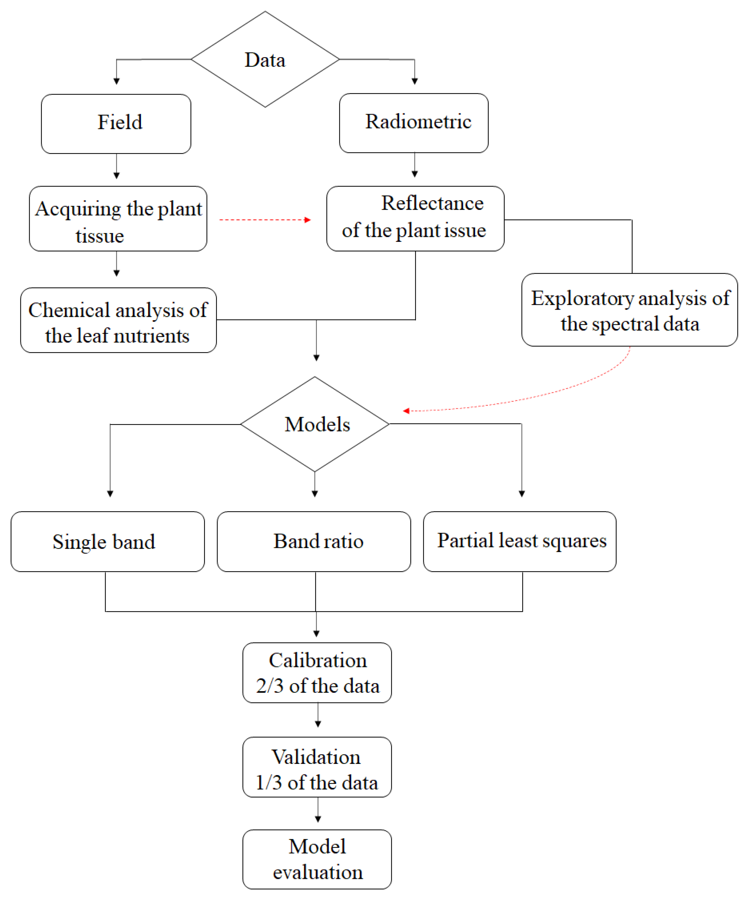
2. Materials and Methods

The trial was carried out in an experimental area on the Pici Campus of the Federal University of Ceará, (546920 E, 9586497 S) (Figure 1). According to Köppen [33], the climate in the region is classified as tropical rainy (Aw’), with a rainy season during the summer and a dry season during the winter, and average monthly temperatures greater than 18 °C. During the experiment, the minimum, mean and maximum temperatures were 25.9, 27.6 and 28.7 °C, respectively, while the minimum, medium and maximum values for relative humidity were 64.25%, 72% and 81.5%, respectively. The soil in the area has a sandy texture, and the main physical and chemical characteristics are shown in

Table 1. Physical and chemical analysis of the soil in the experimental area.

Attribute	Value
Coarse sand (g.kg−1)	523.00
Fine sand (g.kg−1)	370.00
Silt (g.kg−1)	52.00
Clay (g.kg−1)	55.00
Bulk density (g.cm−3)	1.46
Particle density (g.cm−3)	2.68
pH (water)	6.92
Calcium (mmolc.dm−3)	16.00
Magnesium (mmolc.dm−3)	13.00
Sodium (mmolc.dm−3)	3.00
Potassium (mmolc.dm−3)	1.00
H + Al (mmolc.dm−3)	18.20
Organic carbon (g.kg−1)	7.02
Total nitrogen (g.kg−1)	0.68
Organic matter (g.kg−1)	12.10
Available phosphorus (mg.dm−3)	23.00
C:N ratio	10:1

Source: Physical and chemical analysis of the soil in the experimental area [38].

.

The experimental plots consisted of five plant rows at a spacing of 1.0 m × 0.3 m with a total area of 9.0 m². Two plants were kept per hole, giving a total population of approximately 67,000 plants ha⁻¹. The crop was drip-irrigated every two days, with irrigation suspended at the fruit maturation stage. According to Cardoso et al. [34], the irrigation of Vigna unguiculata (L.) Walp should be suspended during the maturation of the pods. The normal evolution of the crop requires a lack or low availability of water during the final stage of the cycle to avoid the grain rotting or the appearance of diseases.

To better explain the processes used in the methodology, a flowchart was created containing the steps adopted in the study (Figure 2).

The crop was fertilised using a standard treatment, including N (urea), P (single superphosphate) and K (potassium chloride) in mineral form, which was defined based on the soil analysis and crop requirements, as per the manual of recommendations and liming for the state of Ceará [35]. In addition, the crop was fertilised with organic compost at doses of 100%, 200% and 300%, where the organic fertiliser was defined based on the nitrogen from the mineral treatment, i.e., 100% of the organic compost contained the same amount of nitrogen as the mineral treatment. Nutrient availability from the organic compost was determined using the equation proposed by [36] and modified by [37].

The crop cycle of Vigna unguiculata (L.) Walp is composed of ten phenological stages, five vegetative and five reproductive stages. The vegetative stages are: Start of germination (V0); Cotyledons level with the soil (V1); Expanded primary leaves (V2); First trifoliate leaf (V3); and Third trifoliate leaf (V4), respectively. The reproductive stages are: Flower bud formation (R5); Opening of the first flower (R6); Appearance of pods (R7); First full pods (R8) and Physiological maturity (R9), respectively, defined by Dourado Neto and Fancelli [39]. The leaf samples were collected at stages V4 (third fully open composite leaf), R6 (at least 50% of open flowers) and R9 (pod maturation). According to Embrapa [34], the most critical stages of Vigna unguiculata (L.) Walp correspond to the stage that precedes flowering, the flowering stage and the grain-filling stage, i.e., stages V4, R6 and R9, respectively.

The leaves were always collected at the same time (08:00 a.m. to 11:00 a.m.). The radiometric readings were taken at the Laboratory of Spectroradiometry of the Federal University of Ceará immediately after collection. The samples were then dried in an oven at 65 °C to constant weight and used for mineral analysis.

To acquire the radiometric data, the FieldSpec 3 Hi-Res spectroradiometer was used (Figure 3). This has a field of view of 25° and operates in the region of 350 to 2500 nm, with a spectral resolution of 3 nm at 700 nm, 8.5 nm at 1400 nm, and 6.5 nm at 2100 nm. The sensor resamples the data to 1 nm, giving a total of 2151 bands. The readings were carried out in a darkroom, thereby eliminating interference from external radiation that might compromise the results. The sensor was positioned at the nadir, 7 cm away from the samples. As a light source, a 250 W halogen lamp was used, with a parabolic reflector, a beam collimated along the target plane and a 30° zenith angle of illumination. A high-reflectance, white Spectralon plate was used to calibrate the sensor. Five readings were taken from each leaf sample; the data were later processed using the ViewSpec Pro software and analysed with an electronic spreadsheet.

After eliminating any non-representative measurements, the mean radiance was calculated. The values for spectral radiance were converted into bidirectional reflectance factors as per Equation (1):

$${\mathrm{FRB}}_{\mathsf{\lambda }}=\frac{{\mathrm{La}}_{,\mathsf{\lambda }}}{{\mathrm{Lr}}_{,\mathsf{\lambda }}}$$

(1)

where:

• FRB_λ = bidirectional reflectance factor (dimensionless)
• La_,λ = spectral radiance of the target (W cm⁻² sr⁻¹ μm⁻¹)
• Lr_,λ = spectral radiance of the reference plate (W cm⁻² sr⁻¹ μm⁻¹).

Oven-dried leaf samples were ground and used to determine the levels of P, K, Ca and Zn. For this, 0.5 g of each sample were submitted to nitroperchloric digestion, as per [41]. The extracts were then suitably diluted to determine the levels of P, K, Ca and Zn in an inductively coupled plasma optical emission spectrometer (ICP-OES).

A descriptive analysis was carried out of the leaf nutrient content for each treatment of the phenological stages under evaluation. Using the radiometric data, a spectral-response graph for the phenological stages measured in the field (V4, R6 and R9) was then generated using the mean values and standard deviation from the descriptive analysis.

The Kolmogorov–Smirnov test was carried out to verify whether the data had a normal distribution.

The models were tested using a single band, the ratio of two bands and partial least squares regression (PLSR) (Figure 2). To select the bands used in the study, a simple correlation analysis was carried out between the spectral data and the nutrient content obtained from the leaf analysis. The bands with the highest correlations were then selected.

A 2D-correlation graph was generated to select the significant bands to be used in the band ratio, employing a statistical tool for testing collinearity [42] available from the online platform of the Brazilian National Institute for Space Research (INPE).

Two-dimensional correlation is a statistical technique that allows the correlation between a dependent variable and various independent variables to be quantified. According to Ogashawara [42], this technique is commonly applied when estimating biogeochemical parameters by means of spectral data, where the use of correlation graphs is an important tool in band selection, reinforced by using hyperspectral sensors. This technique was used by Ogashawara [42] to select the best Normalised Difference Indices in order to estimate soil texture.

When carrying out the partial least squares regression, the spectral characteristics from 350 to 399 nm were removed due to the high level of noise. The PLSR was carried out using the Unscrambler^® software, to which values for the reflectance factor of each wavelength (X) and the variable response values (Y) referring to the nutrient content of Vigna unguiculata (L.) Walp was added.

Of the total number of data employed, 2/3 were used to calibrate the models, and 1/3 for validation [43]. To evaluate the performance of the models, the coefficient of determination (R²), root mean square error (RMSE) and the residual prediction deviation (RPD) were used. Equation (2) shows the expression for the RMSE, while Equation (3) refers to the RPD.

$$\mathrm{RMSE}=\sqrt{\frac{\mathsf{Ʃ} {({\mathrm{Y}}_{\mathrm{i}}-\mathrm{Y})}^2 }{\mathrm{n}}}$$

(2)

where:

• Y_i = measured values
• Y = predicted values
• n = sample size

$$\mathrm{RPD}=\sqrt{\frac{\mathrm{REFERENCE} \mathrm{STANDARD} \mathrm{DEVIATION} }{\mathrm{RMSE}}}$$

(3)

3. Results and Discussion

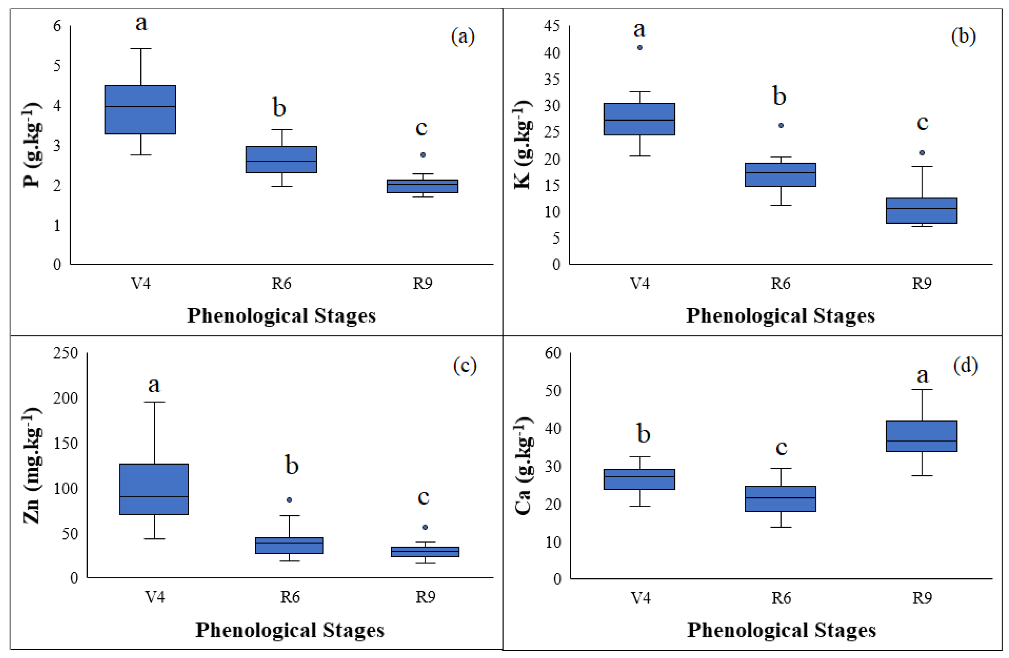
3.1. Nutrient Content

The levels of P, K and Ca (Figure 4) fall within the ranges considered adequate for full crop development [44], with values ranging from 2.5 to 5.0 g.kg⁻¹ for phosphorus, 8.0 to 50.0 g.kg⁻¹ for potassium and 8.0 to 30.0 g.kg⁻¹ for calcium. These ranges are an indication of the nutritional status of the plant, where values less than those recommended represent a nutritional deficiency with a consequent need for correction, while greater values indicate toxicity [44,45].

During the cycle of Vigna unguiculata (L.) Walp, the levels of P, K and Zn in the leaves decrease, while the Ca content remains steady or increases (Figure 4). This can partly be explained by the differential translocation of these nutrients, where calcium is hardly translocated by the phloem [46] and tends to accumulate in the leaves during plant development. A reduction in the other nutrients under evaluation may be a consequence of their translocation from the leaves to the reproductive parts of the plant.

As a nutrient, P is necessary during each phenological stage of the crop, especially the early stages, since its limitation can restrict plant development [47]. The nutrient acts by increasing cells [46] and is mostly absorbed during the pre-flowering stage; however, according to [48], as the crop develops, the P content is reduced.

There is an antagonistic relationship between K and Ca, in which one element affects the absorption of the other [49]. The greatest requirement for Ca at phenological stage R9 (Figure 4c) is related to pod fixation, where, due to the antagonism between the two nutrients, the K content is reduced (Figure 4b).

Zinc (Zn) is an essential micronutrient for plant nutrition [50]. It influences plant and root growth, is involved in many metabolic pathways and allows the photosynthetic area to expand [51]. As such, it is mainly required during the early stages of the plant and decreases as the crop cycle progresses (Figure 4d).

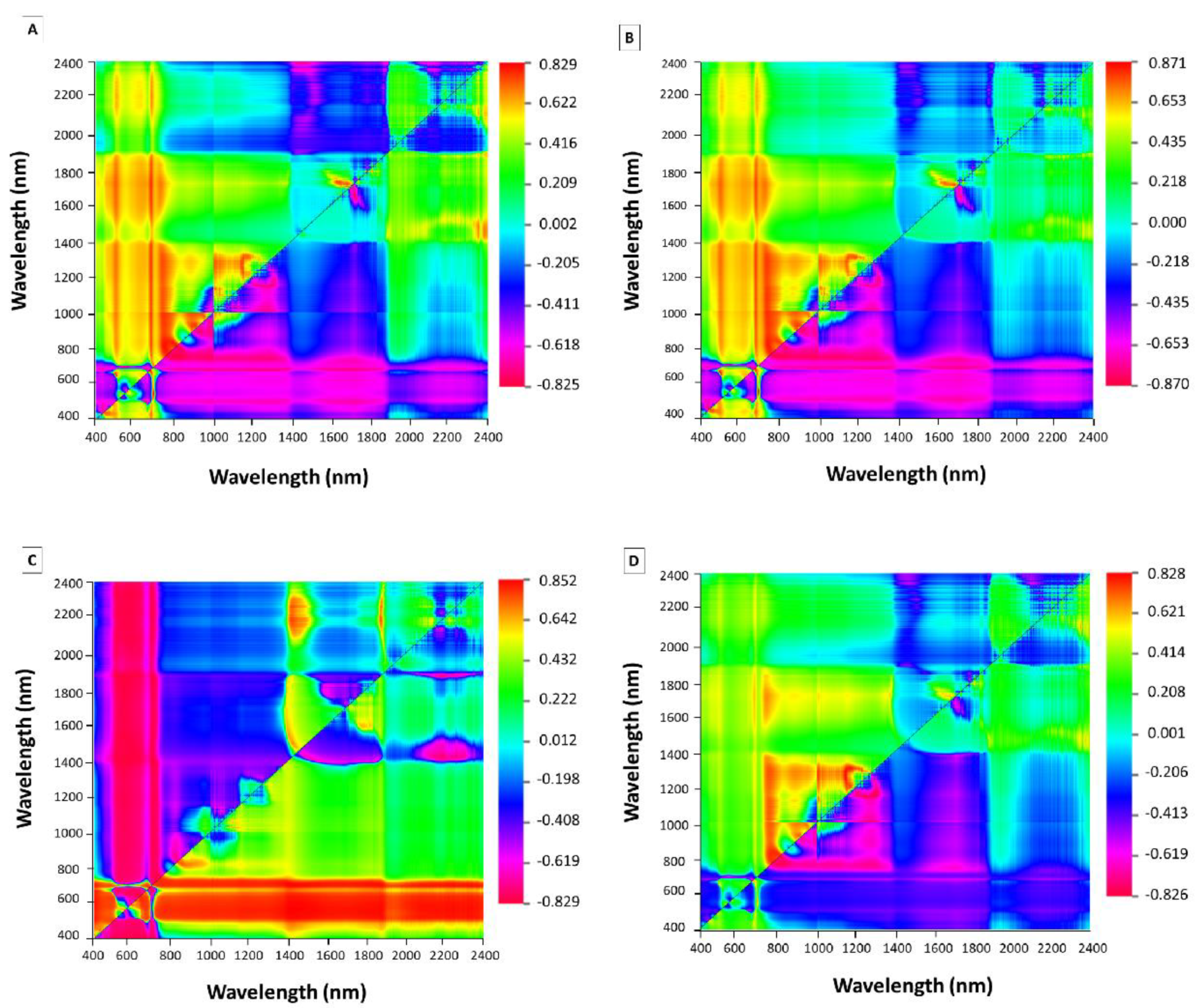
3.2. Spectral Reflectance

The spectral properties of a leaf are a function of its chemical composition, morphology and internal structure [52]. Nutrient functions in plant physiology influence the spectral reflectance of the leaves. Each phenological stage of the crop was registered by spectral reflectance curves typical of healthy green vegetation [53], with reflectance values that differed only slightly (Figure 5). The reduction in plant nutrient content promotes greater leaf reflectance by significantly affecting the optical properties of the leaf [54]. A small difference in leaf nutrient values, which are lower at the R9 stage, reveals a slight change in reflectance.

In the visible region, the vegetation presented, in the three phenological stages studied, lower reflectance factors when compared to the infrared region, with absorption valleys observed in the blue (490 nm) and red (680 nm). The study conducted by [55] is in accord with this result, affirming that the strong light absorption by pigments dominates the properties of the green leaf in the visible spectrum. Pigments that interfere heavily in reflectance are chlorophyll, carotenes and xanthophylls. In the visible region, there is an interaction between radiant energy and the foliar structure by means of absorption and spread, where it is selectively absorbed by the chlorophyll and converted into heat or fluorescence, being photochemically stored in the form of organic components [56].

At stage R9, there is an increase in reflectance in the visible region (Figure 5C) of approximately 20% compared to the other stages. This is due to the senescence of the plants, which have lower levels of chlorophyll and reduce radiation absorption by these pigments [57]. Similar results were obtained by [58] in the common bean, where the reflectance peak near 550 nm increased as the crop reached the end of the cycle.

In the near-infrared (700 to 1000 nm), there is a small absorption of radiation; on the other hand, there is large internal radiation spread in the leaf, in which mesophyll structures have a major influence on reflectance [59]. Water availability is a factor that can also interfere in leaf reflectance in this region because it can cause alterations in the water—air relationship in the mesophyll. Reflectance peaks can be seen in the near-infrared region during each phenological stage of the study, caused by low EMR absorption (970 and 1180 nm) and spread within the foliar structures [60]. In this region, the mean reflectance was 0.5 (Figure 5). In the NIR, no great variations in reflectance were observed in the plants in the different phenological stages, considering that throughout the entire cycle, the crop presented no water or nutritional stress that might have caused alterations in the cellular structure of the cowpea leaf.

In the SWIR (1000 to 2400 nm), crop reflectance is more influenced by water [61]. A reduction in water quantity leads to a degradation of proteins and photosynthesising pigments, which restricts the absorption of electromagnetic radiation and, consequently, results in increased reflectance in this region. At the wavelengths of 1450 and 1930 nm, well-marked valleys can be observed, indicating the presence of water in the leaf (Figure 5). One can see that the valleys at 1450 and 1930 nm are quite accentuated, which indicates the presence of water. During crop development, there were hardly any alterations in this region because irrigation continued throughout the cycle and was suspended only in phase R9; nevertheless, no alterations in reflectance were observed in this phenological stage, indicating that the reading was taken prior to the plant showing signs of water deficit.

P plays a part in the process of producing energy for photosynthesis [62]. A reduction in the levels of this nutrient leads to a reduction in chlorophyll efficiency, resulting in increased reflectance in the visible region, as occurs in plants in the process of senescence.

Like P, K is included in the process of energy production and has a role in activating the ATPase enzyme, forming ATP [63]. Stein [64] found that wavelengths, which are important for predicting this nutrient in leaves, are located in the visible and red-edge regions.

Ca participates in the transfer of electrons from photosystem II to photosystem I, i.e., it helps to increase leaf chlorophyll, and as a result, increases absorption in the visible region [65].

Zn is involved in the activity of the superoxide dismutase enzyme that increases photosynthetic activity in the plant [66]. This nutrient is correlated with wavelengths between 680 and 720 nm, located in the red-edge region, as discussed in [67].

3.3. Model Calibration

3.3.1. Single Band

The values for the Pearson correlation coefficient (Figure 6) between the reflectance values and the P, K, Ca and Zn content in the leaves (Figure 5) show the wavelengths with the highest correlation and that were later selected to construct the empirical models for estimating the nutrient content in the leaves of Vigna unguiculata (L.) Walp (Figure 6).

It can be seen that the values of the correlation coefficients for Zn were not sufficient for any wavelength on the spectrum. It was, therefore, not possible to create an empirical model for estimating this nutrient using a single band.

An analysis of Figure 6 shows the wavelengths for which there was a greater correlation between the leaf content of each element and the reflectance factors.

Table 2. Models for estimating leaf nutrient content using a single spectral band.

Nutrient	Wavelength (nm)	Equation	R2
P	684	y = −89.297x + 8.158	0.62
K	684	y = −915.51x + 74.546	0.63
Ca	720	y = 208.12x − 41.659	0.67

shows the selected wavelengths together with the calibration and validation equations and R² values.

As discussed in Section 3.2 above, the visible region is strongly influenced by the pigments present in the leaf, especially chlorophyll. Near 700 nm, there is a point known as the red edge, which is the limit of the chlorophyll absorption process, and where scattering begins in the internal structures of the leaves [68]. Chu [69] show that the band from 650 to 750 nm (red edge) is essential for understanding reflectance based on biochemical changes in the plant. In creating the models, at least one wavelength was selected from each of these two regions (visible and red edge), as they are somehow related to chlorophyll.

Researchers studying the estimation of the nutrient content of leaves using single-band models had good results when selecting wavelengths located in the visible region [70,71]. On the other hand, [56] found high negative correlations (R² = −0.7) between the phosphorus content and spectral reflectance, especially from 1400 to 1900 nm, which contradicts the result found in this study.

3.3.2. Band Ratio

Based on the highest 2D-correlation coefficients (Figure 7), two wavelengths were selected to develop the estimation models. The wavelengths used to carry out the band ratio, as well as the calibration equations and R² values, are shown in

Table 3. Models for estimating leaf nutrient content using spectral band ratios.

Nutrient	Band Ratio (nm)	Equation	R2
P	826/750	P = 34.63x − 32.35	0.66
K	744/816	K = −256.09x + 265.54	0.70
Ca	720/844	Ca = 89.675x − 33.934	0.63
Zn	1252/1148	Zn = 6818.2x − 6643	0.66

.

It can be seen that most of the models used to predict elements using one band or the two-band ratio selected wavelengths located in the red-edge and near-infrared bands. According to [72], selecting wavelengths in these two regions improves the accuracy of the estimate. Selecting wavelengths around 680 nm for phosphorus and potassium is related to the participation of these nutrients in the processes of producing energy for photosynthesis. According to Yen Mee [73], strong absorption of the chlorophyll pigment occurs around 680 nm.

Another region with strong chlorophyll absorption is close to 740 nm [73]. This wavelength was selected for calcium due to the contribution of the nutrient to an increase in leaf chlorophyll.

The wavelengths selected to obtain the models for estimating the P, K and Ca content are located in the near-infrared (NIR) region. Furthermore, although it is more suitable for detecting organic compounds, the NIR is also able to extract information about the inorganic fraction of leaf samples, such as Ca, K and other micronutrients [74].

3.3.3. Partial Least Squares Regression (PLSR)

Using reflectance data from the cowpea, models were tested that aimed to estimate the leaf nutrient content at stages V4, R6 and R9 individually, as well as a single model tested using joint data from all three stages. The bands selected to generate the models for estimating the nutrient content in the leaves of Vigna unguiculata (L.) Walp are shown in

Table 4. Spectral bands selected for calibrating the PLSR models.

Phenological Stage	Nutrient	Band	n	Adjusted R2
V4	Ca	413, 625, 1301, 1405, 1683, 1714, 1726, 1727, 1883, 1904	16	0.98
	Zn	634, 1364, 1981, 1994	16	0.73
R6	Zn	923, 925, 944, 951, 1864, 1890	17	0.90
R9	K	630, 1405	17	0.43
	Ca	613, 631, 1350	17	0.59
All (V4, R6, R9)	P	504, 651, 685, 1649, 1715	50	0.77
	K	504, 651, 685, 1715, 1735	50	0.84
	Ca	705, 1890, 2377	50	0.73
	Zn	751, 1715, 2434	50	0.57

n: Number of data used to calibrate the models.

and the calibration equations in

Table 5. Equations used in calibrating the PLSR models.

Phenological Stage	Nutrient	Equation
V4	Ca	Ca = 41.380740 − 10.38684 λ1683 nm − 3.63733 λ1405 nm + 1.344476 λ413 nm + 4.155283 λ1883 nm − 9.864286 λ1726 nm − 7.38664·λ1714 nm − 7.014894 λ1031 nm + 5.896256 λ1904 nm − 10.20575 λ1727 nm + 2.19506·λ625 nm
	Zn	Zn = −607.617 − 10181.2 λ634 nm + 3809.383 λ1364 nm + 2204.323 λ1994 nm − 3493.65 λ1981 nm
R6	Zn	Zn = −119.164400 + 70.25752 λ944 nm + 71.05573 λ951 nm + 71.56557 λ1890 nm + 88.90969 λ1864 nm + 68.28416 λ925 nm + 67.71706 λ923 nm
R9	K	K = −1.65418 − 80.7834 λ630 nm + 116.8171 λ1405 nm
	Ca	Ca = 106.346000 − 252.393 λ1350 nm + 3637.852 λ631 nm − 3048.85 λ613 nm
All the bands together (V4. R6. R9)	P	P = 6.162487 − 124.4690 λ685 nm + 181.6616 λ651 nm − 87.4141 λ504 nm + 299.9536 λ1715 nm − 293.5019 λ1649 nm
	K	K = 8.754299 − 427.4241 λ685 nm + 2012.5704 λ651 nm − 1940.1794 λ504 nm + 2668.3838 λ1715 nm − 2624.0833λ1735 nm
	Ca	Ca = 16.96427 + 193.3209 λ705 nm − 670.447 λ2377 nm + 458.5386 λ1890 nm
	Zn	Zn = −92.4856 + 1803.0171 λ1715 nm − 2073.2190 λ2434 nm − 519.7374 λ751 nm

PLSR: Partial least squares regression; V4: Vegetative stage 4; R6: Reproductive stage 6; R9: Reproductive stage 9; λ: reflectance factor.

.

The models tested for the individual phenological stages (Table 4) did not select any useful bands for predicting the levels of each of the nutrients evaluated in this study. However, when using the data from the three stages together, it was possible to select a considerable number of bands to construct the model for each nutrient.

Analysing Table 4, it can be seen that in the PLSR models obtained for predicting P, wavelengths located in both the visible region and the NIR intervals that are influenced by this nutrient were selected. P is an important macronutrient, as it is involved in the metabolic processes of plants [73], being a part of protein and lipid molecules. The spectral regions most affected by these compounds are located between 350 and 1500 nm and from 2350 to 2500 nm [74]. Furthermore, P also participates in the processes of producing energy for photosynthesis [62], as it is strongly influenced by wavelengths in the visible region.

In the present study, only one wavelength was selected in the range mentioned by [74]; the remaining wavelengths selected by the PLSR models are mostly in the visible region (Table 4). K is strongly related to carbohydrates and organic acids and can be measured indirectly using these compounds in the near-infrared region [75]. Disagreeing with the results obtained in this study, Prananto [74] states that regions of the electromagnetic spectrum most strongly affected by carbohydrates are found roughly between 1000 and 1500 nm and from 1950 to 2300 nm.

The PLSR models selected few wavelengths in the near-infrared, while the greatest number of wavelengths for obtaining the Ca estimation model were selected at the V4 stage. As a macronutrient, Ca is strongly related to leaf structure; on the electromagnetic spectrum, this region is located in the near-infrared, between 700 and 1500 nm. Unlike the present results, Aldana [76] states that Ca compounds bind to plant cells that are sensitive in the NIR region.

Analysing Table 4, few of the models obtained in this study selected wavelengths within the range of 680 to 720 nm, which may have contributed to the low efficiency of the models in estimating the zinc content. Zn is a micronutrient for the life cycle of plants and carries out various metabolic activities. In their research, Shao [67] states that Zn is correlated with the red-edge wavelengths (680 to 720 nm); however, their results are different from those found in the present study.

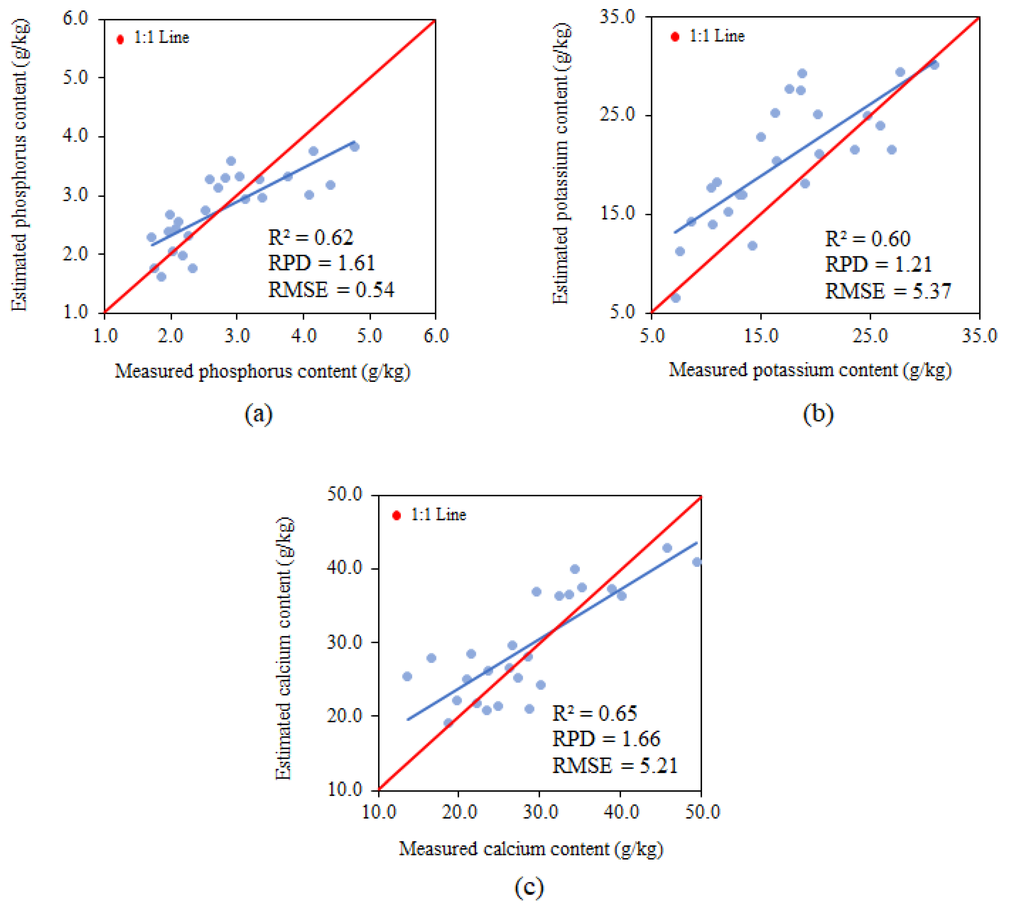
3.4. Model Validation

From the work data, two-thirds of the samples were selected for model calibration, while the final third was set aside for the validation phase. The validation process for the models was conducted using the following statistical metrics: coefficient of determination (R²), Root Mean Square Error (RMSE) and the Residual Prediction Deviation (RPD).

The parameters used for analysing model fit for the variable phosphorus using a single band presented an R² of 0.62, RPD of 1.61 and RMSE of 0.54 g.kg⁻¹, classifying them as moderate for R² and RMSE and satisfactory for RPD (Figure 8a). The phosphorus estimate tends to underestimate the values of this nutrient.

The parameters used for analysing the model fit for the variable potassium using a single band presented an R² of 0.60, RPD of 1.21 and RMSE of 5.37 g.kg⁻¹, classifying them as moderate for R² and insufficient for RPD and RMSE (Figure 8b). The potassium estimate tends to underestimate all values of this nutrient.

The parameters used for analysing model fit for the variable calcium using a single band presented an R² of 0.65, RPD of 1.66 and RMSE of 5.21 g.kg⁻¹, classifying them as moderate for R², satisfactory for RPD and insufficient for RMSE (Figure 8c). The calcium estimate tends to underestimate all predicted values. Despite the model underestimating the concentrations, it presents the same trend; that is, underestimating the lower and higher values of calcium.

According to Ge [77], the models used for predicting phosphorus and calcium are highly accurate; however, the RMSE of the model for estimating calcium is insufficient, electing the model for estimating phosphorus as the most reliable among the single-band models.

Model performance using band ratios for estimating phosphorus presented an R² of 0.60, RPD of 1.52 and RMSE of 0.65 g.kg⁻¹, classified as moderate for R² and satisfactory for RPD and RMSE (Figure 9a).

Model performance using band ratios to estimate potassium presented an R² of 0.68, RPD of 1.67 and RMSE of 5.02 g.kg⁻¹, classified as moderate for R² and satisfactory for RPD and RMSE (Figure 9b).

Model performance using band ratios for estimating calcium presented an R² of 0.67, RPD of 1.63 and RMSE of 5.42 g.kg⁻¹, classified as moderate for R² and satisfactory for RPD and RMSE (Figure 9c).

Model performance using band ratios for estimating zinc presented an R² of 0.57, RPD of 1.50 and RMSE of 30.63 g.kg⁻¹, classified as moderate for R² and satisfactory for RPD and RMSE (Figure 9d).

Using band ratios allowed for the obtainment of predictive models for each of the nutrients studied; however, the best-fitted model was the one used to estimate phosphorus. Nutrient estimates tend to overestimate lower values and underestimate higher values. RMSE values for zinc prediction are excessively high compared to other nutrients. Liao [78] confirms that micronutrient predictions are generally not as good as those reported for macronutrients.

Using samples from all phenological stages as a set, the model using band ratios also proved to be efficient only in predicting phosphorus content using selected bands, with an R² of 0.60, RPD of 1.62 and RMSE of 0.65 g.kg⁻¹.

The parameters used for analysing the model performance for the variable calcium using PLSR in phenological stage V4 presented an R² of 0.78, RPD of 1.10 and RMSE of 3.10 g.kg⁻¹, classifying them as moderate for R² and insufficient for RPD and RMSE (Figure 10a). The calcium estimate tends to overestimate all values for this nutrient.

The parameters used for analysing model performance for the variable zinc using PLSR in phenological stage V4 presented an R² of 0.97, RPD of 1.40 and RMSE of 31.60 g.kg⁻¹, classifying them as strong for R², satisfactory for RPD and insufficient for RMSE (Figure 10b). The zinc estimate tends to overestimate all zinc values.

The parameters used for analysing model performance for the variable zinc using PLSR in phenological phase R6 presented an R² of 0.58, RPD of 0.60 and RMSE of 24.60 g.kg⁻¹, classifying them as moderate for R² and insufficient for RPD and RMSE (Figure 11). The zinc estimate tends to underestimate all zinc values.

The parameters used for analysing model performance for the variable potassium using PLSR in phenological phase R9 presented an R² of 0.82, RPD of 0.60 and RMSE of 6.40 g.kg⁻¹, classifying them as strong for R² and insufficient for RPD and RMSE (Figure 12a). The potassium estimate tends to overestimate values up to 10.0 g.kg⁻¹ and underestimate values over 10.0 g.kg⁻¹.

The parameters used for analysing model performance for the variable calcium using PLSR in phenological phase R9 presented an R² of 0.61, RPD of 1.00 and RMSE of 6.20 g.kg⁻¹, classifying them as moderate for R² and insufficient for RPD and RMSE (Figure 12b). The calcium estimate tends to overestimate values up to 40.0 g.kg⁻¹ and underestimate values over 40.0 g.kg⁻¹.

The performance of the model using PLSR with data from all phenological phases utilised for the estimate of phosphorus presented an R² of 0.74, RPD of 1.66 and RMSE of 0.47 g.kg⁻¹, classified as moderate for R² and satisfactory for RPD and RMSE (Figure 13a).

The performance of the model using PLSR with data from all phenological phases utilised for estimating potassium presented an R² of 0.77, RPD of 2.06 and RMSE of 3.38 g.kg⁻¹, classified as moderate for R² and insufficient for RPD and RMSE (Figure 13b).

The performance of the model using PLSR with data from all phenological phases utilised for estimating calcium presented an R² of 0.66, RPD of 1.54 and RMSE of 4.67 g.kg⁻¹, classified as moderate for R², satisfactory for RPD and insufficient for RMSE (Figure 13c).

The performance of the model using PLSR with data from all phenological phases utilised for estimating zinc presented an R² of 0.80, RPD of 1.66 and RMSE of 30.57 g.kg⁻¹, classified as moderate for R², satisfactory for RPD and insufficient for RMSE (Figure 13d).

With the exception of the model for estimating zinc, the others presented a trendline similar to the 1:1 line.

Comino [79] also verified the inefficiency of partial least squares regression models used to estimate the zinc content due to the high RMSE value, similar to that found in the present study. However, better correlations can be obtained when the nutrient content is higher. The partial least squares regression model is a powerful means of multivariate analysis for predicting leaf nutrients [22,27,75,76]. On the other hand, the PLSR models for the individual phenological stages are unreliable when estimating leaf nutrients. According to Campelo [40], the amount of data used to predict the models influences the results; this explains the better performance of the models tested using joint data from all three phenological stages.

The best model selected using data from all phenological stages together was the one using PLSR to estimate phosphorus content, with an R2 of 0.74, RPD of 1.66 and RMSE of 0.47. The selection of the band improved the model performance in the three methodologies applied. The models constructed using PLSR became reliable following the selection of the band utilising data from all phenological stages as a set but still needs to be fitted to predict micronutrients, such as zinc.

In a study with compacted alfalfa samples, [29] achieved respective RPD values of 3.6, 3.4, 3.1 and 2.9 for estimating the P, K, Ca and Zn content, which are different to the results obtained in this study, where an RPD value of 1.66 was found for P, values of between 0.6 and 2.06 for K, between 1.00 and 1.54 for Ca and between 0.36 and 1.66 for Zn. Using PLSR to predict the nutrient content of the dendê leaf, measuring the reflectance with a spectroradiometer, [80] obtained R² values of between 0.49 and 0.90 for predicting phosphorus, and values ranging from 0.61 to 0.85 and from 0.69 to 0.86 for estimating potassium and calcium, respectively, agreeing with the results of the present study (P: 0.77, K: 0.84 and Ca: 0.73). When using PLSR to estimate nutrients in woody plant species, [81] obtained RPD values of 2.3 and 3.8, respectively, for predicting P and Ca, unlike the results of this study, which resulted in lower RPD values (1.66 for P, and between 1.10 and 1.54 for Ca).

4. Conclusions

The use of reflectance data obtained by spectroscopy allows for the quantification of nutrient content; however, the degree of precision of the models varies according to the phenological stage of the crop and the quantity of data utilised, being more precise with a greater quantity of information and with the utilisation of data from all stages studied. The partial least squares regression associated to the spectroscopy shows the great potential for the development of predictive models of nutrients in Vigna unguiculata (L.) Walp.

The bands located in the visible and near-infrared regions seemed promising for estimating nutrient content in the leaves of Vigna unguiculata (L.) Walp. The estimate of zinc content in the leaves did not generate satisfactory results and presented low predictive potential.

The technique for predicting nutrient content in leaves provides faster results for monitoring the nutritional needs of the crop since it does not require laboratory analyses, generation of residues and does not require removal of a large quantity of plant material, hence, it allows the nutritional correction of the crop quickly and easily, reducing the possible harm that can come from nutritional imbalance.

References

1. Muñoz-Amatriaín, M.; Mirebrahim, H.; Xu, P.; Wanamaker, S.I.; Luo, M.; AlHakami, H.; Alpert, M.; Atokple, I.; Batieno, B.J.; Boukar, O.; et al. Genome resources for climate-resilient cowpea, an essential crop for food security. Plant J. 2017, 89, 1042–1054. [Google Scholar] [CrossRef] [PubMed] [Green Version]
2. Carvalho, M.; Lino-Neto, T.; Rosa, E.; Carnide, V. Cowpea: A legume crop for a challenging environment. J. Sci. Food Agric. 2017, 97, 4273–4284. [Google Scholar] [CrossRef] [PubMed]
3. Lonardi, S.; Muñoz-Amatriaín, M.; Liang, Q.; Shu, S.; Wanamaker, S.I.; Lo, S.; Tanskanen, J.; Schulman, A.H.; Zhu, T.; Luo, M.; et al. The genome of cowpea (Vigna unguiculata L. Walp.). Plant J. 2019, 98, 767–782. [Google Scholar] [CrossRef] [Green Version]
4. Freire Filho, F.R. Feijão-Caupi No Brasil: Produção, Melhoramento Genético, Avanços e Desafios; Embrapa Meio-Norte: Teresina, Brazil, 2011; 84p. [Google Scholar]
5. Andrade Júnior, A.S.D.E. Cultivo do Feijão-Caupi (Vigna unguiculata (L.) Walp.); Embrapa Mid-North: Brasília, Brazil, 2002. [Google Scholar]
6. Bertini, C.H.; Do Vale, J.C.; Borém, A. Feijão-caupi do Plantio à Colheita; Editora UFV: Viçosa, Brazil, 2017. [Google Scholar]
7. Campanharo, M.; Monnerat, P.H.; Espindula, M.C.; Rabello, D.S. Doses De Níquel Em Feijão Caupi Cultivado Em Dois Solos. Rev. Caatinga 2013, 26, 9. [Google Scholar]
8. Li, Q.; Jin, C.; Wang, G.; Ji, J.; Guan, C.; Li, X. Enhancement of endogenous SA accumulation improves poor-nutrition stress tolerance in transgenic tobacco plants overexpressing a SA-binding protein gene. Plant Sci. 2020, 292, 110384. [Google Scholar] [CrossRef]
9. Malmir, M.; Tahmasbian, I.; Xu, Z.; Farrar, M.B.; Bai, S.H. Prediction of macronutrients in plant leaves using chemometric analysis and wavelength selection. J. Soils Sediments 2020, 20, 249–259. [Google Scholar] [CrossRef]
10. Osco, L.P.; Ramos, A.P.M.; Moriya, É.A.S.; de Souza, M.; Junior, J.M.; Matsubara, E.; Imai, N.N.; Creste, J.E. Improvement of leaf nitrogen content inference in Valencia-orange trees applying spectral analysis algorithms in UAV mounted-sensor images. Int. J. Appl. Earth Obs. Geoinf. 2019, 83, 101907. [Google Scholar] [CrossRef]
11. Abdulridha, J.; Batuman, O.; Ampatzidis, Y. UAV-Based Remote Sensing Technique to Detect Citrus Canker Disease Utilizing Hyperspectral Imaging and Machine Learning. Remote Sens. 2019, 11, 1373. [Google Scholar] [CrossRef] [Green Version]
12. Calou, V.B.C.; Teixeira, A.D.S.; Moreira, L.C.J.; Lima, C.S.; de Oliveira, J.B.; de Oliveira, M.R.R. The use of UAVs in monitoring yellow sigatoka in banana. Biosyst. Eng. 2020, 193, 115–125. [Google Scholar] [CrossRef]
13. Osco, L.P.; Ramos, A.P.M.; Pinheiro, M.M.F.; Moriya, É.A.S.; Imai, N.N.; Estrabis, N.; Ianczyk, F.; De Araújo, F.F.; Liesenberg, V.; Jorge, L.A.D.C.; et al. A Machine Learning Framework to Predict Nutrient Content in Valencia-Orange Leaf Hyperspectral Measurements. Remote Sens. 2020, 12, 906. [Google Scholar] [CrossRef] [Green Version]
14. Peng, Z.; Guan, Z.; Liao, Y.; Lian, S. Estimating total leaf chlorophyll content of Gannan navel orange leaves using hyper-spectral data based on partial least squares regression. IEEE Access 2019, 7, 155540–155551. [Google Scholar] [CrossRef]
15. Zheng, H.; Li, W.; Jiang, J.; Liu, Y.; Cheng, T.; Tian, Y.; Zhu, Y.; Cao, W.; Zhang, Y.; Yao, X. A Comparative Assessment of Different Modeling Algorithms for Estimating Leaf Nitrogen Content in Winter Wheat Using Multispectral Images from an Unmanned Aerial Vehicle. Remote Sens. 2018, 10, 2026. [Google Scholar] [CrossRef] [Green Version]
16. O’Connell, J.; Byrd, K.; Kelly, M. Remotely-Sensed Indicators of N-Related Biomass Allocation in Schoenoplectus acutus. PLoS ONE 2014, 9, e90870. [Google Scholar] [CrossRef]
17. Oliveira, M.; Queiroz, T.R.G.; Teixeira, A.D.S.; Moreira, L.C.J.; Leão, R.A.D.O. Reflectance spectrometry applied to the analysis of nitrogen and potassium deficiency in cotton. Rev. Ciência Agronômica 2020, 51. [Google Scholar] [CrossRef]
18. Chen, Z.; Wang, X. Model for estimation of total nitrogen content in sandalwood leaves based on nonlinear mixed effects and dummy variables using multispectral images. Chemom. Intell. Lab. Syst. 2019, 195, 103874. [Google Scholar] [CrossRef]
19. Fletcher, R.S.; Reddy, K. Random forest and leaf multispectral reflectance data to differentiate three soybean varieties from two pigweeds. Comput. Electron. Agric. 2016, 128, 199–206. [Google Scholar] [CrossRef]
20. Rokhafrouz, M.; Latifi, H.; Abkar, A.A.; Wojciechowski, T.; Czechlowski, M.; Naieni, A.S.; Maghsoudi, Y.; Niedbała, G. Simplified and Hybrid Remote Sensing-Based Delineation of Management Zones for Nitrogen Variable Rate Application in Wheat. Agriculture 2021, 11, 1104. [Google Scholar] [CrossRef]
21. Pullanagari, R.; Kereszturi, G.; Yule, I. Mapping of macro and micro nutrients of mixed pastures using airborne AisaFENIX hyperspectral imagery. ISPRS J. Photogramm. Remote Sens. 2016, 117, 1–10. [Google Scholar] [CrossRef]
22. Wen, P.-F.; He, J.; Ning, F.; Wang, R.; Zhang, Y.-H.; Li, J. Estimating leaf nitrogen concentration considering unsynchronized maize growth stages with canopy hyperspectral technique. Ecol. Indic. 2019, 107, 105590. [Google Scholar] [CrossRef]
23. Yu, X.; Lu, H.; Liu, Q. Deep-learning-based regression model and hyperspectral imaging for rapid detection of nitrogen concentration in oilseed rape (Brassica napus L.) leaf. Chemom. Intell. Lab. Syst. 2018, 172, 188–193. [Google Scholar] [CrossRef]
24. De Oliveira, D.M.; Fontes, L.M.; Pasquini, C. Comparing laser induced breakdown spectroscopy, near infrared spectroscopy, and their integration for simultaneous multi-elemental determination of micro- and macronutrients in vegetable samples. Anal. Chim. Acta 2019, 1062, 28–36. [Google Scholar] [CrossRef]
25. Ling, B.; Goodin, D.G.; Raynor, E.; Joern, A. Hyperspectral Analysis of Leaf Pigments and Nutritional Elements in Tallgrass Prairie Vegetation. Front. Plant Sci. 2019, 10, 142. [Google Scholar] [CrossRef] [PubMed] [Green Version]
26. Abdel-Rahman, E.M.; Mutanga, O.; Odindi, J.; Adam, E.; Odindo, A.; Ismail, R. Estimating Swiss chard foliar macro- and micronutrient concentrations under different irrigation water sources using ground-based hyperspectral data and four partial least squares (PLS)-based (PLS1, PLS2, SPLS1 and SPLS2) regression algorithms. Comput. Electron. Agric. 2017, 132, 21–33. [Google Scholar] [CrossRef]
27. Mao, H.; Gao, H.; Zhang, X.; Kumi, F. Nondestructive measurement of total nitrogen in lettuce by integrating spectroscopy and computer vision. Sci. Hortic. 2015, 184, 1–7. [Google Scholar] [CrossRef]
28. Gama, T.; Wallace, H.; Trueman, S.; Tahmasbian, I.; Bai, S. Hyperspectral imaging for non-destructive prediction of total nitrogen concentration in almond kernels. Acta Hortic. 2018, 1219, 259–264. [Google Scholar] [CrossRef]
29. González-Martín, I.; Hernández-Hierro, J.M.; González-Cabrera, J.M. Use of NIRS technology with a remote reflectance fibre-optic probe for predicting mineral composition (Ca, K, P, Fe, Mn, Na, Zn), protein and moisture in alfalfa. Anal. Bioanal. Chem. 2007, 387, 2199–2205. [Google Scholar] [CrossRef]
30. Galvez-Sola, L.; Garciasanchez, F.J.; Pérez-Pérez, J.G.; Gimeno, V.; Navarro, J.M.; Moral, R.; Nicolas, J.J.M.; Nieves, M. Rapid estimation of nutritional elements on citrus leaves by near infrared reflectance spectroscopy. Front. Plant Sci. 2015, 6, 571. [Google Scholar] [CrossRef] [Green Version]
31. Halgerson, J.; Sheaffer, C.; Martin, N.; Peterson, P.; Weston, S. Nearinfrared reflectance spectroscopy prediction of leaf and mineral concentrations in alfalfa. Agron. J. 2004, 96, 344–351. [Google Scholar]
32. Yarce, C.J.; Rojas, G. Near infrared spectroscopy for the analysis of macro and micro nutrients in sugarcane leaves. Sugar Ind. 2012, 137, 707–710. [Google Scholar] [CrossRef]
33. Köppen, W. Climatologia: Con un Estudio de los Climas de la Tierra; Fondo de Cultura Economica: Mexico City, Mexico, 1948; 478p. [Google Scholar]
34. Cardoso, M.J.; Bastos, E.A.; Andrade Junior, A.S.; De Athayde Sobrinho, C. Feijão-Caupi: O Produtor Pergunta, a Embrapa Responde; Embrapa: Brasília, Brazil, 2017; 244p. [Google Scholar]
35. Aquino, A.B.; Aquino, B.F.; Hernandez, F.F.F.; Holanda, F.J.M.; Freire, J.M.; Crisóstomo, L.A.; Costa, R.I.; Unchôa, S.C.P.; Fernandes, V.L.B. Recomendações de Adubação e Calagem para o Estado do Ceará; UFC: Fortaleza, Brazil, 1993; 247p. [Google Scholar]
36. Furtini Neto, A.E.; Vale, F.R.; Resende, A.V.; Guilherme, L.R.G.; Guedes, G.A.A. Fertilidade do Solo; UFLA: Lavras, Brazil, 2001; 261p. [Google Scholar]
37. SILVA, C.A. Uso de resíduos orgânicos na agricultura. In Fundamentos da Matéria Orgânica do solo: Ecossistemas Tropicais e Subtropicais, 2nd ed.; Métropole: Porto Alegre, Brazil, 2008; pp. 597–624. [Google Scholar]
38. Magalhães, A.C.M. de Adubação orgânica Com Base na taxa de Mineralizaçãode Nutrientes do Composto Orgânico. Master’s Thesis, Universidade Federal do Ceará, Fortaleza, Brazil, 2018. [Google Scholar]
39. Dourado Neto, D.; Fancelli, A.L. Produção de Feijão; Agropecuária: Guaíba, Brazil, 2000; 385p. [Google Scholar]
40. Campelo, D.H. Uso do Sensoriamento Remoto Para Diagnóstico Nutricional na Cultura do Milho Irrigado. Ph.D. Thesis, Universidade Federal do Ceará, Fortaleza, Brazil, 2018; 182p. [Google Scholar]
41. Silva, F.C. da (Org.). Manual de Análises Químicas de Solos, Plantas e Fertilizante; Embrapa Comunicação para Transferência de Tecnologia: Brasília, Brazil, 1999. [Google Scholar]
42. Ogashawara, I.; Curtarelli, M.P.; Souza, A.F.; Augusto-Silva, P.B.; Alcântara, E.H.; Stech, J.L. Interactive Correlation Environment (ICE)—A Statistical Web Tool for Data Collinearity Analysis. Remote Sens. 2014, 6, 3059–3074. [Google Scholar] [CrossRef] [Green Version]
43. Lopes, F.B.; Barbosa, C.C.F.; Novo, E.M.L.D.M.; de Carvalho, L.A.S.; de Andrade, E.M.; Teixeira, A.D.S. Modelling chlorophyll-a concentrations in a continental aquatic ecosystem of the Brazilian semi-arid region based on remote sensing. Revista Ciência Agronômica 2021, 52, 1–12. [Google Scholar] [CrossRef]
44. Wilcox, G.E.; Fageria, N.K. Deficiências Nutricionais do feijão, sua Identificação e Correção; Boletim Técnico, 5; Embrapa/CNPAF: Goiânia, Brazil, 1976; 22p. [Google Scholar]
45. Martinez, H.E.P.; Menezes, J.F.S.; De Souza, R.B.; Venegas, V.H.A.; Guimarães, P.T.G. Faixas críticas de concentrações de nutrientes e avaliação do estado nutricional de cafeeiros em quatro regiões de Minas Gerais. Pesqui. Agropecuária Bras. 2003, 38, 703–713. [Google Scholar] [CrossRef] [Green Version]
46. Marschner, P. Marschner’s Mineral Nutrititon of Higher Plants, 3rd ed.; Academic Press: Cambridge, MA, USA, 2012; 649p. [Google Scholar]
47. Büll, L.T.; Novello, A.; Corrêa, J.; Boas, R. Doses de fósforo e zinco na cultura do alho em condições de casa de vegetação; Bragantia: Campinas, Brazil, 2008; Volume 67, pp. 941–949. [Google Scholar]
48. Zucareli, C. Adubação fosfatada, produção e desempenho em campo de sementes de feijoeiro CV. Carioca Precoce e IAC Carioca Tybatã. Master’s Thesis, Universidade Estadual Paulista, Botucatu, Brazil, 2005. Júlio de Mesquita Filho. [Google Scholar]
49. Cavalcante, L.F.; Santos, C.J.O.; De Holanda, J.S.; De Lima Neto, A.J.; De Souto, A.G.L.; Dantas, T.A.G. Produção de maracujazeiro Amarelo no solo Com Calcário e Potássio sob Irrigação com água Salina; Irriga: Botucatu, Brazil, 2018; Volume 23, pp. 727–740. [Google Scholar]
50. Malavolta, E. Manual de Nutrição Mineral de Plantas; Editora Agronômica Ceres: São Paulo, Brazil, 2006; p. 638. [Google Scholar]
51. Pedrosa, M.V.B. Qualidade Fisiológica de Sementes de Feijão (Stageolus vulgaris L.) em Função da Maturação e Adubação Com enxofre, Nitrogênio e Zinco. Master’s Thesis, Universidade Federal do Espírito Santo, Vitória, Brazil, 2017; p. 87. [Google Scholar]
52. Ponzoni, F.J.; Shimbukuro, Y.E.; Kuplich, T.M. Sensoriamento Remoto da Vegetação. São José dos Campos, 2nd ed.; Oficina de Textos: Sao paulo, Brazil, 2012; 176p. [Google Scholar]
53. Moreira, M.A. Fundamentos do Sensoriamento Remoto e Metodologias de Aplicação, 4th ed.; Viçosa, M.G., Ed.; UFV: Abbotsford, BC, Canada, 2011; 422p. [Google Scholar]
54. Gasparotto, A.C.; Nanni, M.R.; Miotto, L.S.; Guirado, G.C.; Silva Junior, C.A.; Silva, A.A.; Cezar, E.; Romagnoli, F. Comportamento espectral de milho submetido a diferentes doses de nitrogênio. XVII Simpósio Brasileiro de Sensoriamento Remoto-SBSR, João Pessoa-PB, Brasil. 2015. Available online: http://marte2.sid.inpe.br/col/sid.inpe.br/marte2/2015/05.31.21.54/doc/@sumario.htm (accessed on 31 October 2021).
55. Liu, L.; Song, B.; Zhang, S.; Liu, X. A Novel Principal Component Analysis Method for the Reconstruction of Leaf Reflectance Spectra and Retrieval of Leaf Biochemical Contents. Remote Sens. 2017, 9, 1113. [Google Scholar] [CrossRef] [Green Version]
56. Carvalho, A. Estudo de Características foliares de Espécies de Lenhosas de cerrado e Sua relação com os Espectros de Reflectância. Ph.D. Thesis, Universidade de Brasília, Brasília, Brazil, 2005. [Google Scholar]
57. Tierny, J.; Vandeborre, J.; Daoudi, M. The Visual Computer. Int. J. Comput. Graphicsv 2008, 24, 155–172. [Google Scholar]
58. Chicati, M.S. Resposta Espectral da Cultura do Feijão e sua Relação com Parâmetros Biofísicos em Diferentes Doses de Nitrogênio/Mônica Sacioto Chicati. Master’s Thesis, Universidade Estadual de Maringá, Maringá, Brazil, 2015. [Google Scholar]
59. Jensen, J.R. Sensoriamento Remoto do Ambiente: Uma Perspectiva em Recursos Terrestres; Parêntese: São José dos Campos, Brazil, 2011; 582p. [Google Scholar]
60. Papa, R.D.A. Comportamento Espectro-Temporal Da Cultura Do Feijão, Por Meio De Dados Obtidos Por Espectroradiometria, Câmera Digital E Imagem Aster; Novas Edições Acadêmicas: Brasília, Brazil, 2009; 146p. [Google Scholar]
61. Moreira, L.C.J.; Teixeira, A.D.S.; Galvao, L. Laboratory Salinization of Brazilian Alluvial Soils and the Spectral Effects of Gypsum. Remote Sens. 2014, 6, 2647–2663. [Google Scholar] [CrossRef] [Green Version]
62. Silva Junior, M.B. Fertilizantes Foliares no Manejo da Mancha de Phoma de Cafeeiro. Master’s Thesis, Universidade Federal de Lavras, Lavras, Brazil, 2013. [Google Scholar]
63. Taiz, L.; Zeiger, E. Fisiologia Vegetal; Artmed: Porto Alegre, Brazil, 2004; pp. 449–484. [Google Scholar]
64. Stein, B.R.; Thomas, V.A.; Lorentz, L.J.; Strahm, B.D. Predicting macronutrient concentrations from loblolly pine leaf reflectance across local and regional scales. GIScience Remote Sens. 2014, 51, 269–287. [Google Scholar] [CrossRef] [Green Version]
65. Gong, X.; Hong, M.; Wang, Y.; Zhou, M.; Cai, J.; Liu, C.; Gong, S.; Hong, F. Cerium Relieves the Inhibition of Photosynthesis of Maize Caused by Manganese Deficiency; Biological Trace Element Research: Clifton, FL, USA, 2011; Volume 141, pp. 305–316. [Google Scholar]
66. Barbosa, M.; Silva, M.; Willadino, L.; Ulisses, C.; Camara, T. Geração e Desintoxicação Enzimática de Espécies Reativas de Oxigênio em Plantas; Ciência Rural: Santa Maria, FL, USA, 2014; Volume 44, pp. 453–460. [Google Scholar]
67. Shao, Y.; He, Y. Visible/Near Infrared Spectroscopy and Chemometrics for the Prediction of Trace Element (Fe and Zn) Levels in Rice Leaf. Sensors 2013, 13, 1872–1883. [Google Scholar] [CrossRef] [PubMed] [Green Version]
68. Curran, P.J.; Dungan, J.L.; Macler, F.A.; Plummer, S.E. The effect of a red leaf pigment on the relationship between red edge and chlorophyll concentration. Remote Sens. Environ. 1991, 35, 69–76. [Google Scholar] [CrossRef]
69. Chu, X.; Guo, Y.; He, J.; Yao, X.; Zhu, Y.; Cao, W.; Cheng, T.; Tian, Y. Comparison of Different Hyperspectral Vegetation Indices for Estimating Canopy Leaf Nitrogen Accumulation in Rice. Agron. J. 2014, 106, 1911–1920. [Google Scholar] [CrossRef]
70. Tian, Y.C.; Yao, X.; Cao, W.X.; Hannaway, D.B.; Zhu, Y. Assessing Newly Developed and Published Vegetation Indices for Estimating Rice Leaf Nitrogen Concentration with Ground- and Space-Based Hyperspectral Reflectance; Field Crops Research: Amsterdam, The Netherlands, 2011; Volume 120, pp. 299–310. [Google Scholar]
71. Abdel-Rahman, E.M.; Ahmed, F.B.; Berg, M.V.D. Estimation of sugarcane leaf nitrogen concentration using in situ spectroscopy. Int. J. Appl. Earth Obs. Geoinf. Enschede 2010, 12, 52–57. [Google Scholar] [CrossRef]
72. Zhou, X.; Huang, W.; Kong, W.; Ye, H.; Luo, J.; Chen, P. Remote estimation of canopy nitrogen content in winter wheat using airborne hyperspectral reflectance measurements. Adv. Space Res. 2016, 58, 1627–1637. [Google Scholar] [CrossRef]
73. Mee, C.Y.; Bala, S.K.; Mohd, A.H. Detecting and Monitoring Plant Nutrient Stress Using Remote Sensing Approaches: A Review. Asian J. Plant Sci. 2016, 16, 1–8. [Google Scholar] [CrossRef]
74. Prananto, J.A.; Minasny, B.; Weaver, T. Near Infrared (NIR) Spectroscopy as a Rapid and Cost-Effective Method for Nutrient Analysis of Plant Leaf Tissues, 1st ed.; Elsevier Inc.: Amsterdam, The Netherlands, 2020; Volume 164, ISBN 9780128207710. [Google Scholar]
75. Clark, D.H.; Mayland, H.F.; Lamb, R.C. Mineral Analysis of Forages with near Infrared Reflectance Spectroscopy 1. Agron. J. 1987, 79, 485–490. [Google Scholar] [CrossRef] [Green Version]
76. De Aldana, B.V.; Criado, B.G.; Ciudad, A.G.; Corona, M.P. Estimation of mineral content in natural grasslands by near infrared reflectance spectroscopy. Commun. Soil Sci. Plant Anal. 1995, 26, 1383–1396. [Google Scholar] [CrossRef] [Green Version]
77. Ge, Y.; Atefi, A.; Zhang, H.; Miao, C.; Ramamurthy, R.K.; Sigmon, B.; Yang, J.; Schnable, J.C. High-throughput analysis of leaf physiological and chemical traits with VIS–NIR–SWIR spectroscopy: A case study with a maize diversity panel. Plant Methods 2019, 15, 1–12. [Google Scholar] [CrossRef] [Green Version]
78. Liao, H.; Wu, J.; Chen, W.; Guo, W.; Shi, C. Rapid diagnosis of nutrient elements in fingered citron leaf using near infrared reflectance spectroscopy. J. Plant Nutr. 2012, 35, 1725–1734. [Google Scholar] [CrossRef]
79. Comino, F.; Ayora-Cañada, M.; Aranda, V.; Díaz, A.; Domínguez-Vidal, A. Near-infrared spectroscopy and X-ray fluorescence data fusion for olive leaf analysis and crop nutritional status determination. Talanta 2018, 188, 676–684. [Google Scholar] [CrossRef]
80. Santoso, H.; Tani, H.; Wang, X.; Segah, H. Predicting oil palm leaf nutrient contents in kalimantan, indonesia by measuring reflectance with a spectroradiometer. Int. J. Remote Sens. 2018, 40, 7581–7602. [Google Scholar] [CrossRef]
81. Petisco, C.; García-Criado, B.; de Aldana, B.R.V.; Zabalgogeazcoa, I.; Mediavilla, S.; García-Ciudad, A. Use of near-infrared reflectance spectroscopy in predicting nitrogen, phosphorus and calcium contents in heterogeneous woody plant species. Anal. Bioanal. Chem. 2005, 382, 458–465. [Google Scholar] [CrossRef] [PubMed]
Figure 1. Location of the experimental area.
Applsci 12 00458 g001
Figure 2. Flowchart of the methodology adopted in the study.
Applsci 12 00458 g002
Figure 3. Geometry of radiometric data acquisition. Source: [40], adapted by the author.
Applsci 12 00458 g003
Figure 4. Nutrient content: phosphorus (a), potassium (b), zinc (c) and calcium (d) in the leaves of Vigna unguiculata (L.) Walp. Different letters indicate a statistical difference by Tukey’s test at 5% probability.
Applsci 12 00458 g004
Figure 5. Mean reflectance spectra and respective standard deviations for each phenological stage: (A) V4, (B) R6 and (C) R9.
Applsci 12 00458 g005
Figure 6. Correlogram between reflectance and the P, K, Ca and Zn content in leaves of Vigna unguiculata (L.) Walp.
Applsci 12 00458 g006
Figure 7. Two-dimensional correlogram between spectral reflectance and the leaf phosphorus (A), potassium (B), calcium (C) and zinc (D) content.
Applsci 12 00458 g007
Figure 8. Relationships between the measured and estimated P (a), K (b) and Ca (c) content, using the single-band model.
Applsci 12 00458 g008
Figure 9. Relationships between the measured and estimated P (a), K (b), Ca (c) and Zn (d) content, using the band-ratio model.
Applsci 12 00458 g009
Figure 10. Relationships between the measured and estimated levels of calcium (a) and zinc (b) at phenological stage V4.
Applsci 12 00458 g010
Figure 11. Relationship between the measured and estimated levels of zinc at phenological stage R6.
Applsci 12 00458 g011
Figure 12. Relationships between the measured and estimated levels of K (a) and Ca (b) at phenological stage R9.
Applsci 12 00458 g012
Figure 13. Relationships between the measured and estimated P (a), K (b), Ca (c) and Zn (d) content using data from all three of the phenological stages (V4, R6 and R9).
Applsci 12 00458 g013