1. Introduction
The power system is experiencing a period of major innovations, most of which are caused by the widespread of both grid-scale and behind-the-meter unpredictable renewable energy sources (RES) and battery energy storage systems (BESS). These new elements are leading to lower reliability and increased uncertainty and variability in the electricity generation, with issues both for the electricity market dynamics and the power system security [
1]. The latter, indeed, is characterized by a higher probability of instability and, sometimes, needs for RES curtailment due to line congestion [
2,
3,
4]. In this framework, demand response (DR) from a multitude of aggregated resources can allow helping the distribution system operator (DSO) in solving contingencies thanks to a change in the prosumers’ behavior [
5,
6,
7,
8]. Ongoing DR programs are characterized by the presence of an aggregator working as a mediator between the prosumer and the DSO, the Transmission System Operator (TSO) or the electrical market manager that manages the aggregated flexible resources to obtain a specific load profile modification. As demonstrated by the scientific literature, aggregators have been present in the DR sector for many years [
9,
10,
11,
12] and, nevertheless, continue to attract great interest from researchers in the field. As an example of the recent literature dealing with aggregators, some papers are proposed below that, although not exhaustive of the topic, give a clear idea on the most discussed issues in the recent literature.
In [
13], the baselining challenge on the interface between the DSO and an aggregator is faced in the context of utilizing flexibility in distribution networks. In [
14], the authors show how an aggregator can fulfill a flexibility request by re-scheduling the home-appliances loads of 20 residential end-users for the next 24-h horizon while minimizing the costs associated with the remuneration given to end-users. The same issue is faced in [
15], where an efficient and scalable MILP/mixed-integer quadratic problem optimization model solved using Gurobi solver, which can handle thousands of appliances, was proposed. In [
16], a scheme was proposed with an aggregator managing the operating power of aggregated air conditioners considering participation priority for voltage regulation purposes, while in [
17], the authors discuss the optimal participation of Electric Vehicles’ aggregators in day-ahead energy and regulation markets, proposing a suitable model for this case. Finally, in [
18], the authors proposed a solution for the interaction of aggregators in a common balancing group consisting of an iterative distributed algorithm based on non-cooperative game theory.
There are not many papers in the literature that deal with the topic of distributed resources aggregation in the absence of an aggregator. As an example, Overgrid is proposed as a P2P architecture designed to control and implement DR schemes in a community of smart buildings in an automatic way [
19], applicable also to the case of small islands [
7]. In [
20], a P2P aggregation platform was proposed for purchasing energy in the liberalized energy market, where prosumers are evaluated and clustered according to their reliability and to the width of the range of regulation allowed. In this context, the Italian research project DEMAND proposed an innovative way for managing the aggregation of prosumers connected to the distribution network without the need of a third-party aggregator and allowing the participation of all kinds of prosumers (industrial, commercial and residential prosumers) [
21,
22].
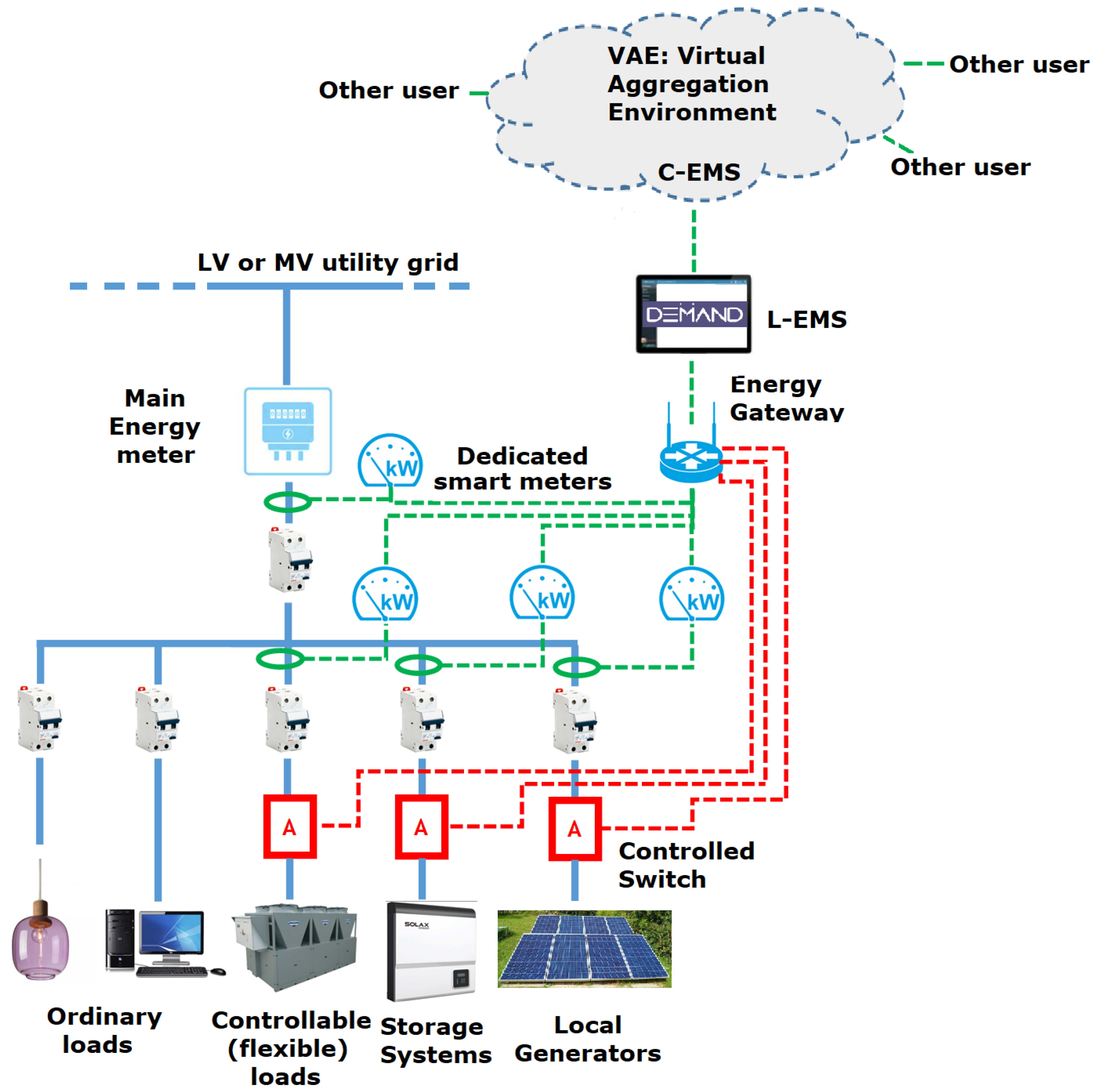
The novelty of DEMAND is the replacement of the physical aggregator with a market platform named Virtual Aggregation Environment (VAE). The VAE is a virtual place that does not take any decision about the aggregation but simply facilitates the exchange of information among the prosumers in a smart grid, with the aim of fostering the combination of their flexibility with a bottom-up approach for providing services to the DSO. The access to the VAE is granted by the energy gateway, an electronic device that every single prosumer of the DEMAND community needs to connect the local Energy Management System (L-EMS) to the cloud EMS (C-EMS), send monitoring data, promise the participation in a DR action and to receive the optimization plan of the local flexible resources.
Figure 1 and
Figure 2 show, respectively, the layout of the system installed at a prosumer’s facility and the interactions between the L-EMS in the energy gateway, the related C-EMS in the Cloud and the VAE.
From the software point of view, the DEMAND system consists of three elements: the L-EMS (which constitutes the energy gateway together with the physical gateway that interfaces with the user’s devices to collect data and to send actuation commands), the remote C-EMS and the platform that facilitates the aggregation of users that is the VAE.
The EMS manages four different phases in the bottom-up aggregation process: configuration, day-ahead management, intra-day management, real-time operation.
The main responsibilities of the L-EMS are:
Forwarding the data received from the physical gateway to the remote EMS;
Translating the optimization plans received from the remote EMS into commands to be sent to the devices through the physical gateway;
Developing a user optimization plan, having a set of basic rules, in case of lack of communication with the remote EMS and, therefore, not being able to participate in an aggregate to respond to the request of the network operator.
The main responsibilities of the remote EMS are:
Enhancing, with an internal optimization process (day-ahead), the availability of user flexibility, to be offered through aggregation with other users in response to a request for flexibility by the network operator;
Determining the aggregate of users and the aggregate offer of flexibility to be proposed to the network operator;
Trying to keep faith with the flexibility promised if the aggregate is chosen by the network operator for the provision of the grid support service requested, and report in time any impossibility (intraday);
Carrying out real-time optimization to ensure the promised flexibility in the offer previously made.
The controlled switches receive digital or analog commands for changing their status (ON/OFF) depending on the device chosen for that function.
The Energy Gateway communicates with the VAE with digital signals.
For understanding the novelty of DEMAND and its potential impact on the exploitation of distributed flexibility, it is important to examine the many solutions and systems for the management of loads and generators connected to the electricity grid that the market offers today. Especially in the industrial and tertiary sectors, these systems generally manage power within microgrids and modulate power absorption or generation towards the DSO. Schneider and Siemens both offer a decentralized SCADA Energy Management System (EMS) to monitor and control loads and generators in order to make the microgrid more efficient, but also to respond to requests from the DSO or energy retailer via OpenADR. General Electric’s Grid IQ Microgrid Control System, ABB’s Micro Grid Controller 600, Toshiba’s µEMS, PSI Smart Telecontrol Unit and Honeywell’s EMS are all very powerful solutions, but essentially proprietary, often working only with devices built by the same manufacturer, inflexible and extremely complex. Open source solutions such as Kiwigrid, Fraunhofer Open Muc and Fraunhofer OGEMA lend themselves well to the implementation of new functions but still have enormous security limitations. None of the solutions mentioned, however, envisages coordination between several users. Distributed logic enabling multi-stakeholder collaboration are not considered. This is due to the fact that these solutions are designed for users whose power consumption/generation levels are already sufficient to guarantee significant effects on the network. All smaller users are excluded from this potential market because they are unable to induce effects on the grid simply by exploiting their limited flexibility. The DEMAND project does not aim to compete with such complex solutions, which are already present in an established market, but to create a solution that enables users to work together, aggregating them in a coordinated and intelligent way, without the need for centralized control. Therefore, the solution will not only be adoptable by industrial and tertiary users, in which it will interface with the internal management systems already present and for which it will represent an innovative extension, but it will also be able to spread to smaller but more numerous residential users.
While a detailed description of the EMS operation has already been presented in previous papers by the same research group [
23,
24], where the potentiality of DEMAND and its main features are described in detail, the present work has the aim to describe in greater detail the operative steps defined for the day-ahead management phase and the formulation of the flexibility economic offer from the prosumer. The paper analyses the information exchange between each prosumer and the VAE, the criteria used for remunerating the prosumers and the actions to be taken to avoid excessive prosumers’ discomfort. In the paper, the algorithm for the management phase is applied to two different case studies: a passive user with only controllable loads and prosumers with controllable loads, photovoltaics and a storage system.
The rest of the paper is structured as follows:
Section 2 contains the description of the algorithm for the day-ahead management phase;
Section 3 reports the cooperative–competitive algorithm for the bottom-up aggregation in the VAE;
Section 4 contains the discussion of two case studies, showing the application of the day-ahead management phase algorithm;
Section 5 reports an assessment of the performance of the aggregation algorithm;
Section 6 contains the conclusion of the work.
2. Day-Ahead Management Phase Algorithm
As described in [
23], during the configuration phase, the EMS forecasts the prosumer’s load diagram for the following day, based on a Monte Carlo approach previously tested for similar applications [
25], and corrected considering the real profiles measured each day. The process leads to the assessment of the flexibility contribution that can be provided by each controllable device in every hour of the following day.
The day-ahead management phase starts when the DSO sends a flexibility request to the VAE. This action activates all EMSes of the prosumers that, according to the DSO information, can participate in the DR action for providing the requested flexibility (e.g., if the flexibility request is the reduction in the power peak downstream a secondary substation, only the EMS of the prosumers supplied by that substation are activated).
Every EMS evaluates and sends to the VAE a list with all the feasible flexibility contributions that the prosumer can provide in the specified time period, indicating, at the same time, the involved flexible devices and the desired tariff (economic offer). The overall flexibility contributions are obtained using the rules of combinatorial calculation by combining the flexible powers associated with each controllable device. If
n is the number of flexible devices and
k is the number of devices combined in order to provide the desired power variation, the number of possible combinations that a given prosumer can offer is:
The total number of combinations is calculated by varying the number of combined devices
k from 1 to
n, therefore:
For each combination of devices and for each potential flexibility contribution, the EMS calculates a flexibility tariff. The tariff T
FL accepted by the prosumer as an adequate remuneration for the service is calculated as:
where DF
t is the disutility function, C
E is the energy price for the prosumer in the specific time interval and
the degradation cost of the batteries used for providing flexibility.
The disutility function is introduced with the aim of taking into account the prosumer’s dissatisfaction due to the change in the forecasted consumption and is given by:
where:
ΔP is the difference between the power consumption that would have been if the prosumer had not participated in the DR action and the power consumption required to satisfy the DR request;
Δt is the time slot of the DR request;
d is the “dissatisfaction cost per kWh”, and it is a parameter that can be set by the prosumer during the configuration phase, depending on the hour of the day and taking into account the prosumer’s habits and preferences.
C
E is given by:
where c is the energy cost expressed in €/kWh. If the energy cost changes during the time slot where the offer is formulated, c is the average of the costs calculated during the time interval
t.
The battery degradation cost is given by:
where C
0 is the purchase and installation cost of the storage system, N
g is the number of charge/discharge cycles of the battery per day for providing flexibility and N
max is the maximum number of charge/discharge cycles during the useful life of the battery.
Once the different couples of flexibility contribution and tariff are assessed, the EMS creates a matrix with all combinations and sends the matrix to the VAE. The day-ahead management procedure is represented in the flow chart in
Figure 3.
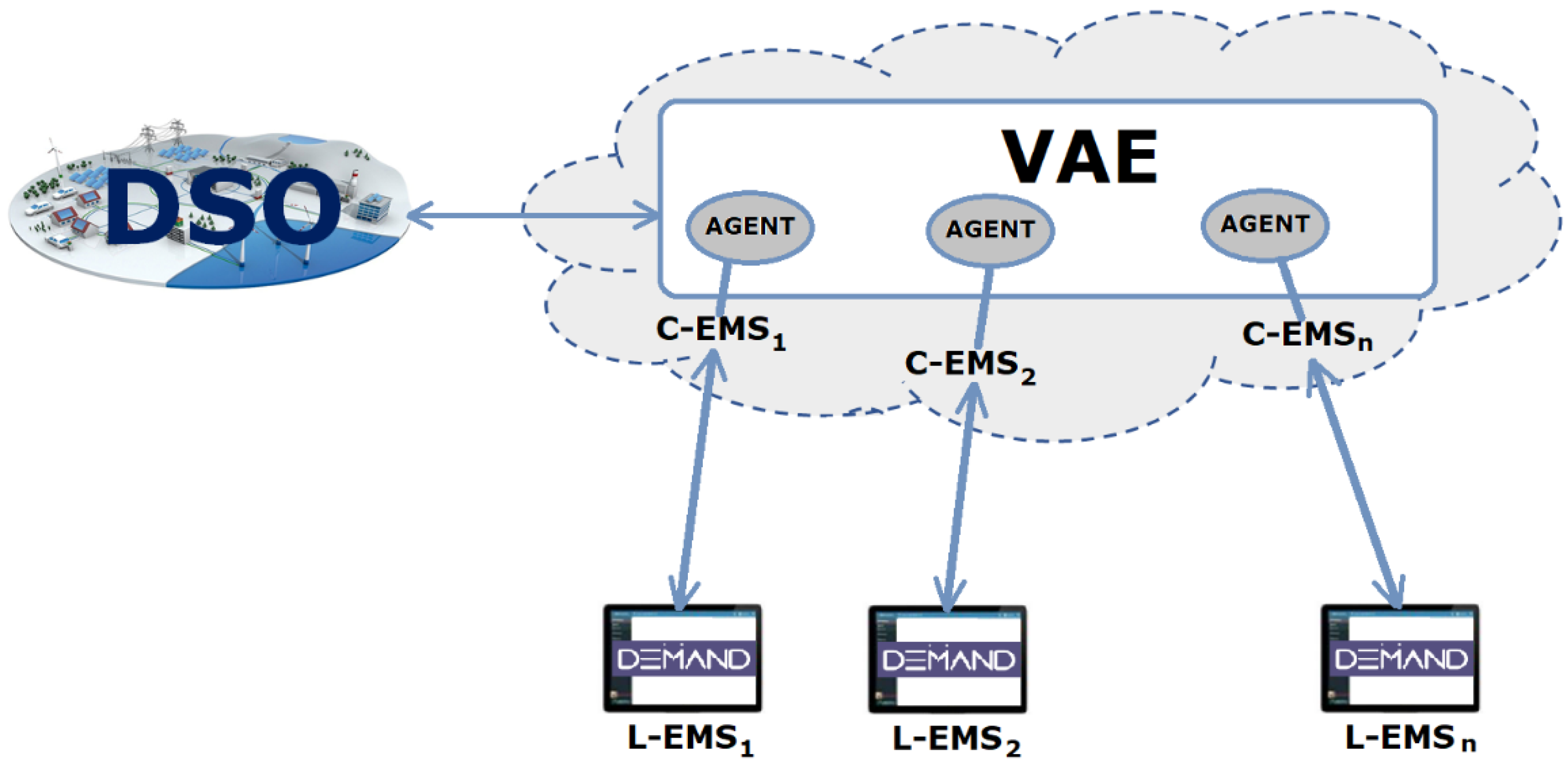
When receiving the matrix of the flexibility couples (power variation–tariff) from each prosumer, the VAE performs a clusterization of the population of the prosumers that have taken part in the aggregation process, based on specific cooperative and competitive algorithms aiming at creating a list of suitable couples of power variation–economic offer for the DSO. As shown in
Section 4, the process can take tens of minutes depending on the number of prosumers and aggregates. The DSO chooses the best offer, assumed as the best compromise between the desired power variation and the most convenient economic offer, and communicates its choice to the VAE. The VAE communicates the result of this process to the EMSes of the winner prosumers that, in this way, provides the flexible service the following day as planned. In particular, each EMS updates the forecasted power profile for taking into account the changes for the flexibility provision and planning a power shifting action for the loads/batteries that provide flexibility. The power shift is, indeed, necessary due to a constraint of the DEMAND system that imposes that the total energy consumption I the day of each prosumer involved in the flexibility provision must not vary. The final step of the day-ahead management phase has the aim of preventing the participation of the prosumers of the winner cluster to more than one winner cluster in the same day, avoiding, in this way, excessive discomfort. This operation is carried out setting to zero the flexibility associated with the devices involved in the winner offer for the rest of the day. Algorithm 1 shows the pseudocode of the algorithm for the EMS operation in the day-ahead phase.
| Algorithm 1 Pseudocode of the algorithm of the day-ahead estimation phase. |
For t = 1 to 144
If the VAE sends a DR request for the time interval t
Calculate all flexibility offers by combining the flexibility of each controllable device;
Calculate the flexibility tariff for each offer;
Communicate the information to the VAE that find the winner cluster of prosumers;
If one of the offers is in the winner cluster
Update the daily load profile;
Update the flexibility values;
End;
Else
t = t + 1;
End;
End. |
3. Bottom-Up Aggregation Algorithm
After evaluating its offer, a prosumer participates in the bottom-up aggregation process. The original bottom-up aggregation algorithm conceived in the context of the DEMAND project implements a collaboration–competition mechanism between electricity prosumers that, activated by the VAE, begin to interact with each other to form aggregates capable of formulating offers that meet the DSO’s request. Within an aggregate, only one user can have leadership. In a nutshell, it is an asynchronous mechanism in which the interaction between the various prosumers can take place while they are in different states. In particular, the possible states are four:
INIT: The prosumer verifies whether it can formulate an offer of flexibility sufficient to satisfy the DSO’s request. If yes, the prosumer goes to state 4; if not, it goes to state 2;
REQUESTER: The prosumer search for other prosumers or aggregates to form an aggregate capable of formulating an offer that responds to the DSO’s request. While staying in this state, the prosumer can receive requests from other prosumers/aggregates (which are in the same REQUESTER state); those requests remain in a queue until the transition to state 3;
RESPONDER: The prosumer examines all requests received, evaluates the potential aggregation results and provides the requested information;
STAND-BY: The prosumer can no longer be contacted because it is part of an aggregate of which it does not hold leadership or is the leader of an aggregate that has made at least one valid offer published on the VAE.
Figure 4 represents the states of each prosumer.
The aggregation process uses some parameters that allow the user to make decisions.
The first parameter is the power reduction coefficient It is defined as the rate, expressed as a percentage, between the power variation that a user (i), if it is the leader of an aggregate, decides to formalize with an offer and the maximum power variation that the same aggregate can provide. In this incremental growth algorithm, the first bids that are formed are those with a limited number of prosumers, each offering the maximum power variation. These bids will be, on average, more expensive than bids that include many prosumers, each with a very small power contribution. It is obvious that the larger the percentage, the faster the prosumer will form an aggregate with a valid offer, the higher the revenue of each individual prosumer that makes up the aggregate, the greater the probability that some other aggregate will create a more advantageous offer (with a lower equivalent price), for example by putting together more prosumers with smaller contributions. Thus, each prosumer will have its own value that it will update based on the success rate of the bids it forms. In particular, could also start at 100% (aggregating prosumers at their maximum power variation) and then could be reduced each time the bid submitted to the VAE is not accepted by the DSO.
The second parameter is the minimum power contribution threshold
It is defined as the limit of its own power variation contribution below, which the prosumer
u(
i), if it is the leader of an aggregate, discards the offer even if valid. This coefficient is connected to the first one since its value influences the minimum value that
can assume during a request of power variation according to the following relation:
The last parameter is the maximum waiting time This parameter is the time that a prosumer (i), if it holds the function of the leader of an aggregate, is willing to wait following the sending of a merge request to another prosumer, leader of another aggregate, before considering that prosumer temporarily unavailable and switching to another prosumer. The maximum waiting time decreases as the frequency of failure (bids not purchased by the DSO) increases.
All bids formulated by the aggregates are ordered based on a score that depends on the criterion by which one bid is rated closer to the DSO’s needs than another. In particular, among bids that meet the DSO’s requirement regarding power variation, those that tend to have the lowest price and the highest reliability will have the highest score. The reliability is assessed as a combination of the reliability coefficients of all the prosumers in an aggregate. Each prosumer, indeed, is characterized by a reliability coefficient that is a number calculated considering all the times it has actually provided the promised flexibility and the times it has failed to meet its commitments.
4. Case Studies
The algorithm for the day-ahead management phase was applied to two different case studies. Both cases refer to a residential prosumer with the same controllable devices, with the difference that in the second case, a photovoltaic (PV) with storage system was present. According to the Italian Standard CEI 0–21 [
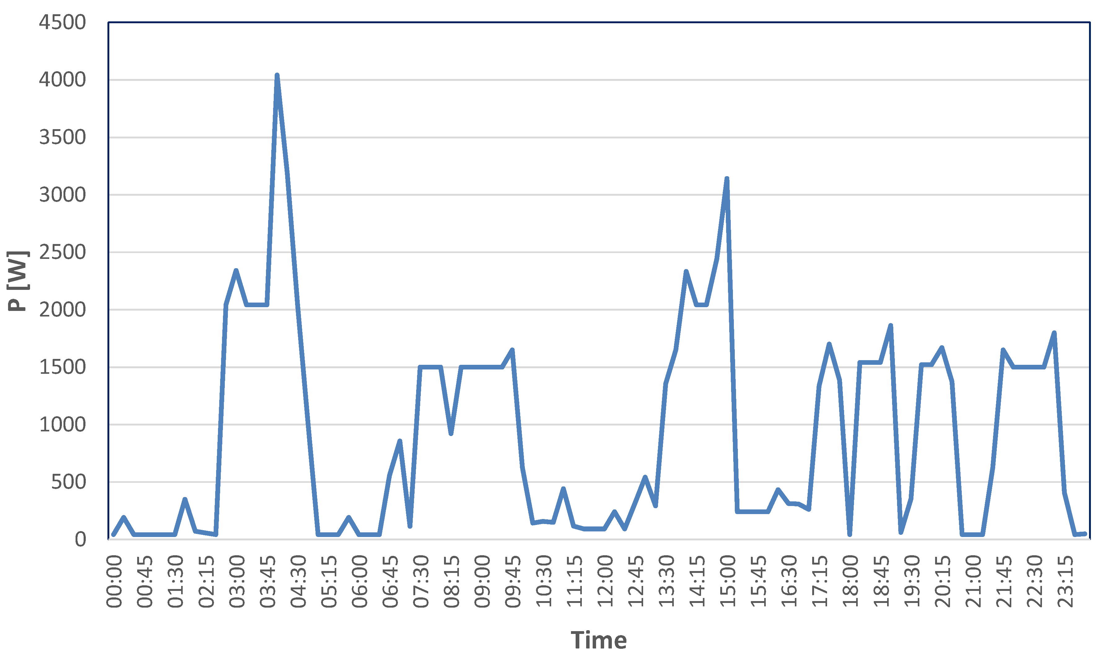
26], the first case is referred to as “passive end-user” because the prosumer has neither a generator nor a storage system, while the second case is referred to as “active end-user”. The power profile of the prosumer (excluded the PV contribution) is forecasted applying a Monte Carlo approach [
27,
28] and is shown in
Figure 5. The flexible devices are:
An electric storage water heater (boiler, maximum power 1.5 kW);
A washing machine (WM, maximum power 2 kW);
A dishwasher (DW, maximum power 2 kW);
A fridge (maximum power 0.3 kW).
Figure 5.
Residential user’s power profile.
Figure 5.
Residential user’s power profile.
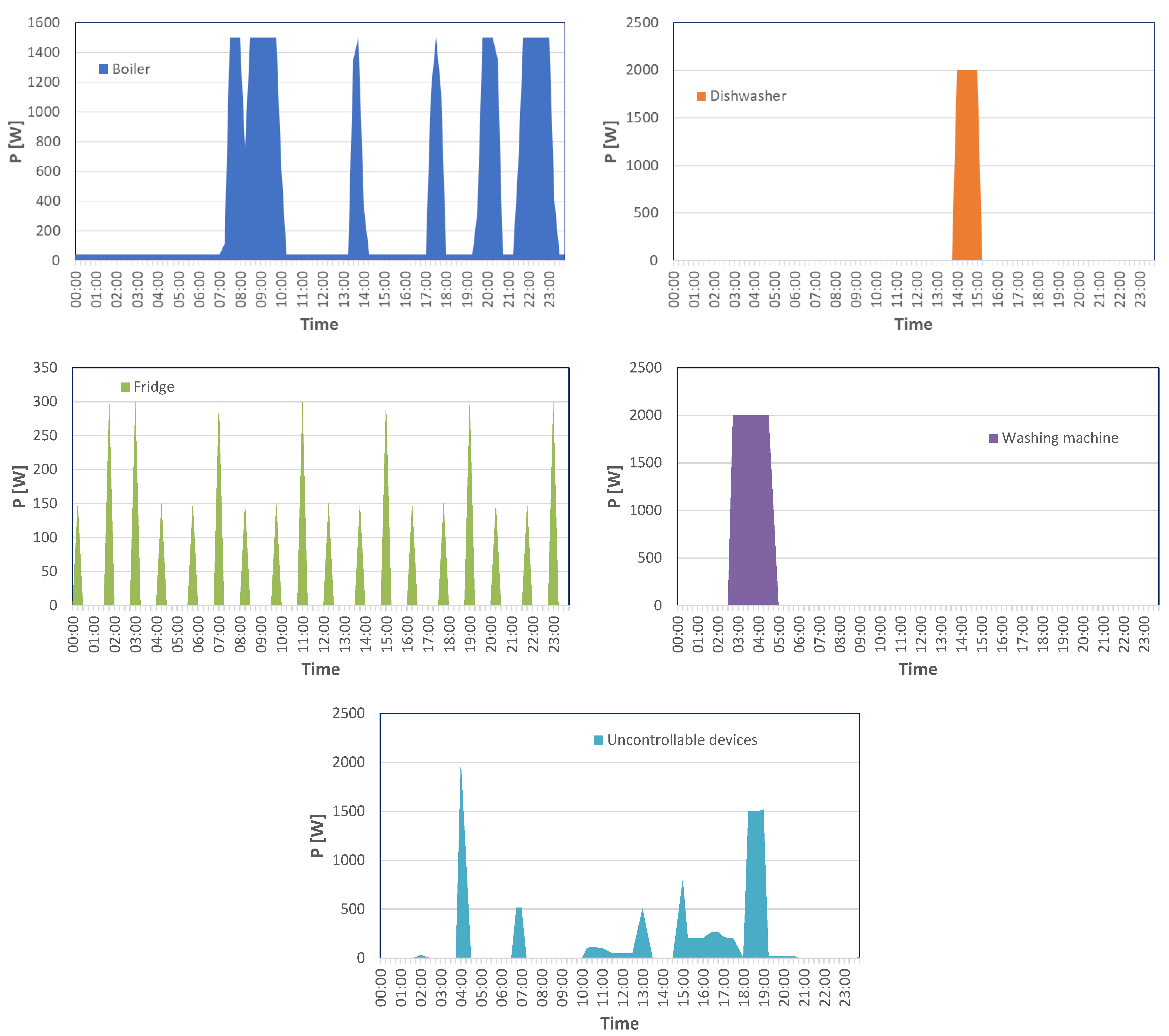
The contribution of each controllable device to the forecasted daily load profile in
Figure 5 is shown in
Figure 6. The figure gives a clear representation of the time interval where the flexible devices are present and can be controlled.
4.1. Case Study 1—Passive User (No PV System, No Batteries)
From the data of the disaggregated load diagram, it is possible to develop the “potential flexibility diagram” for each individual controllable device, which represents the sign and maximum flexibility value that the device can provide at each hour of the day (
Figure 7). Specifically, a positive flexibility value represents the opportunity to increase the prosumer’s instantaneous energy consumption; conversely, a negative one represents the opportunity to decrease the instantaneous energy consumption.
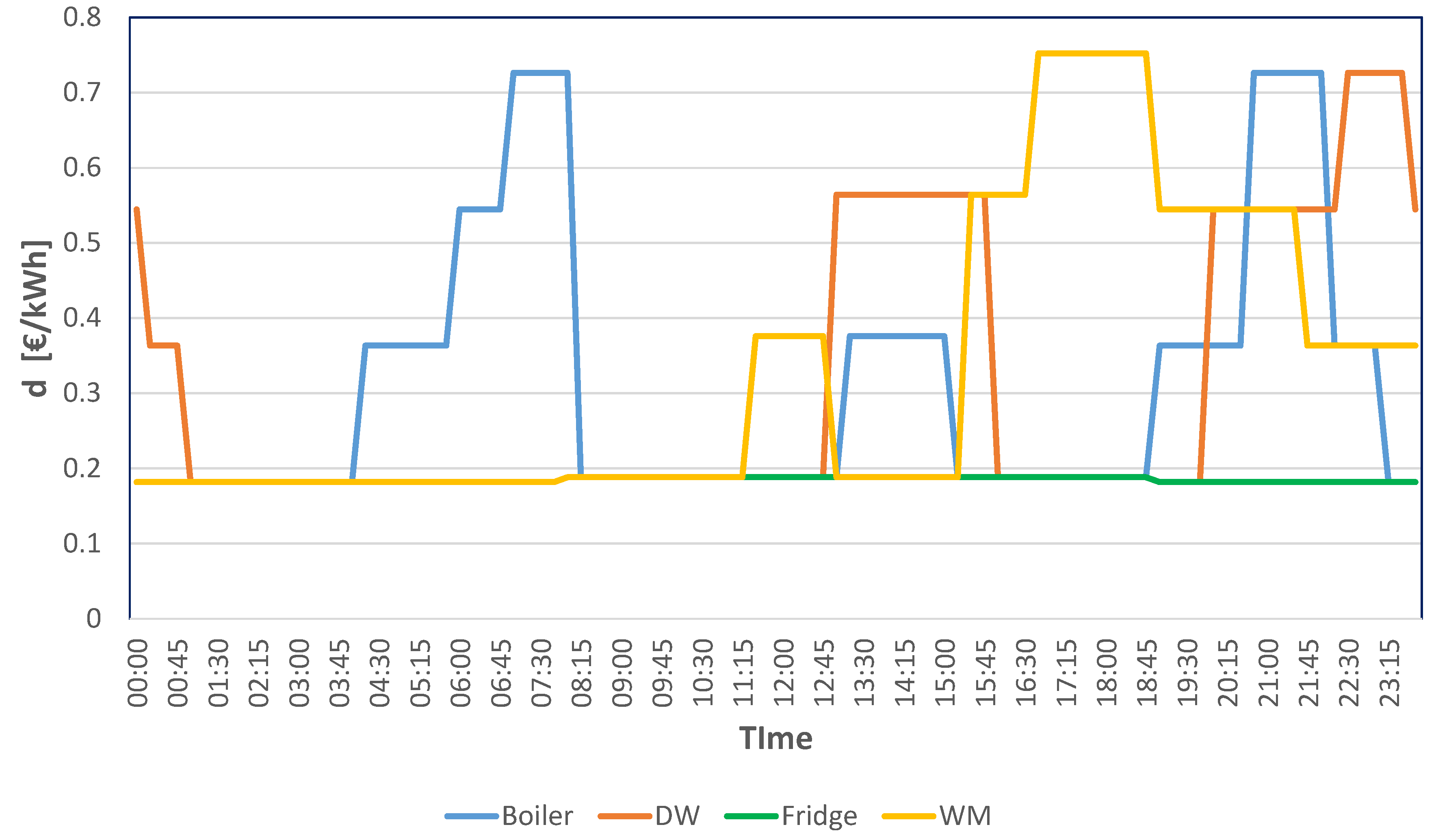
According to a typical Italian double-tariff contract in 2020 for domestic end-users [
29], the energy cost per hour is assumed to equal to 0.188 €/kWh from 8:00 to 19:00 and 0.182 €/kWh in the rest of the day, while the dissatisfaction cost of every controllable device was estimated considering the habits of a typical residential prosumer [
28,
29,
30] and is represented in
Figure 8. It should be emphasized that the way in which the algorithm operates is not influenced by the price of electricity paid by the user. The tariff conditions only influence the economic value of the offer.
The simulation has been carried out considering two different DR requests for the whole day, and in particular:
When the DSO requests a flexibility amount (and the admitted tolerance) to be delivered in a specific time interval, the VAE informs all the EMS that could contribute, and each EMS interested in participating in the provision of the flexibility service communicates to the VAE its power level expected in the time interval indicated by the DSO and elaborates a list of all flexibility offers that the prosumer could produce, including the price of each offer and the IDs of the appliances involved. If the EMS is able to submit independently an offer that satisfies the flexibility request received from the DSO, that offer is presented to the VAE. Otherwise, the aggregation process starts: the EMS interacts with the other EMSes by forming groups or aggregates, each characterized by an overall offer consisting of a variation in power supplied at a given price.
In this simulation, it was hypothesized that the prosumer selected for the winner cluster offers the tuple quantity/price in
Table 1.
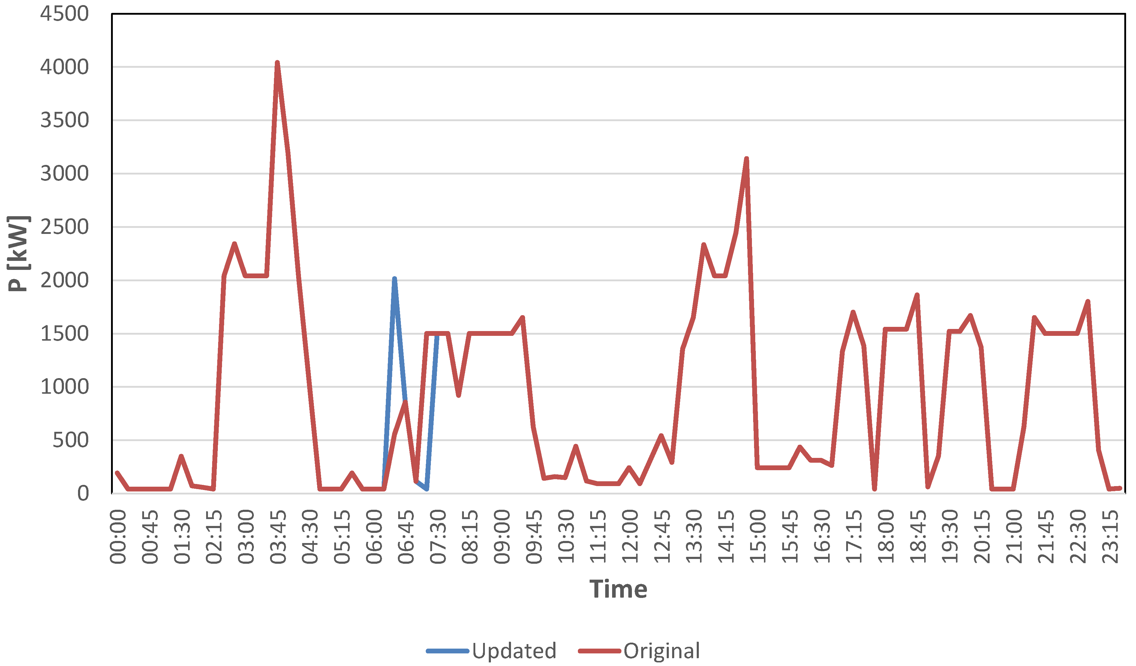
As a consequence, the load diagram is updated considering a load shifting action in a specific time interval, depending on the prosumer’s preferences (
Figure 9). In this case, the load shift interval was supposed to start at 07:30.
At the same time, the potential flexibility diagrams are updated, as shown in
Figure 10, following the criteria described in
Section 2: in the specific case, the flexibility values associated with the boiler are set to zero for the remaining hours of the day.
For the flexibility request at 14:45, the same process is repeated, but with the uploaded input data. At this point, the aggregation algorithms in the VAE are carried out again, and it was supposed that the prosumer had been selected for the winner cluster with the tuple quantity/price in
Table 2.
The load diagram was then updated as shown in
Figure 11, considering a load shift action at 15:15.
Finally, the potential flexibility diagrams were updated, and, in particular, the flexibility values associated with the dishwasher were set to zero for the remaining hours of the day (
Figure 12).
4.2. Case Study 2—Active User (with PV System and Batteries)
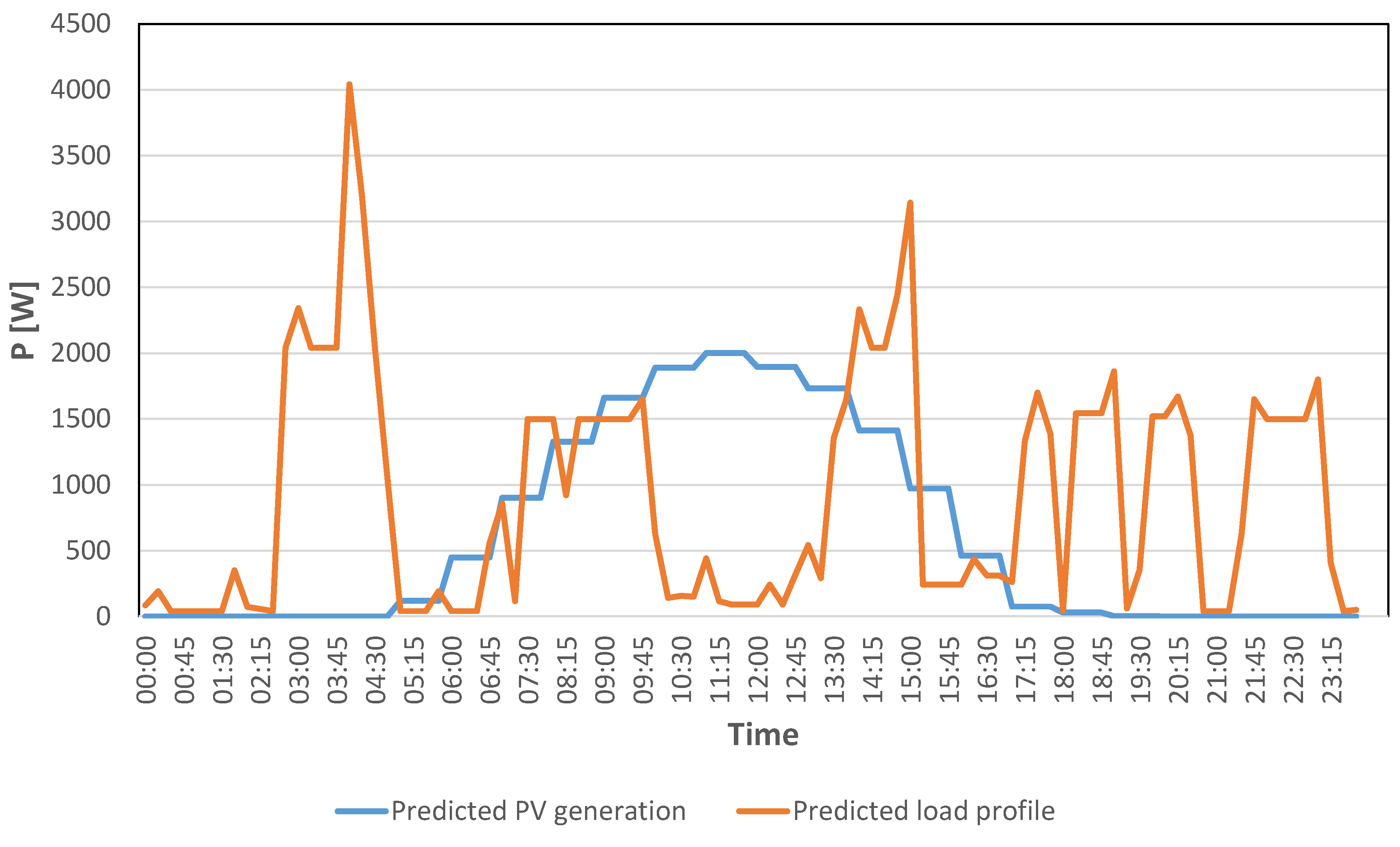
The scenario of the second case study differs from the first one for the presence of a local PV system with a battery storage system. In particular, the production profile forecasted for the day-after is shown in
Figure 13, while le characteristics of the storage system [
31] are reported in
Table 3.
Indicating with E
PV(t) the energy produced by the PV system in the time interval t and with E(t) the energy consumption of the prosumer in the same time interval, when:
the surplus energy E
sto(t), expressed as indicated in (9), will be stored in the battery.
A comparison between the predicted load diagram and the predicted PV production profile allows graphically identifying the time intervals in which energy can be stored in the battery (
Figure 14).
In this case study, the storage system is assumed to be used to provide flexibility by injecting energy into the grid, causing the same effect as a local reduction in electricity demand. The estimated hourly dissatisfaction cost for the storage system is chosen by the prosumer during the configuration phase and can be taken as a multiple of the hourly cost of electricity based on perceived discomfort. In this case, it was set to the minimum value (equal to the cost of electricity: 0.188 €/kWh from 8:00 to 19:00 and 0.182 €/kWh in the rest of the day) because it was considered that using the storage system to provide flexibility causes low discomfort for the prosumer.
In order to calculate the price of bids involving the battery storage system, it is required to calculate the degradation cost using Equation (6) with
:
The simulation is performed considering a request for a decrease in energy consumption in the time interval 12:00–12:15. The prosumer is assumed to be selected for the winning cluster with the quantity/price tuple in
Table 4.
In this case, the price of the winning bid is higher than in case 1, where the storage system is not involved. In fact, although the dissatisfaction cost is lower than the other cases, the contribution of the degradation cost is predominant.
5. Performance of the Bottom-Up Aggregation Process
The aggregation process is tested for various situations to assess the time required for the creation of the aggregates.
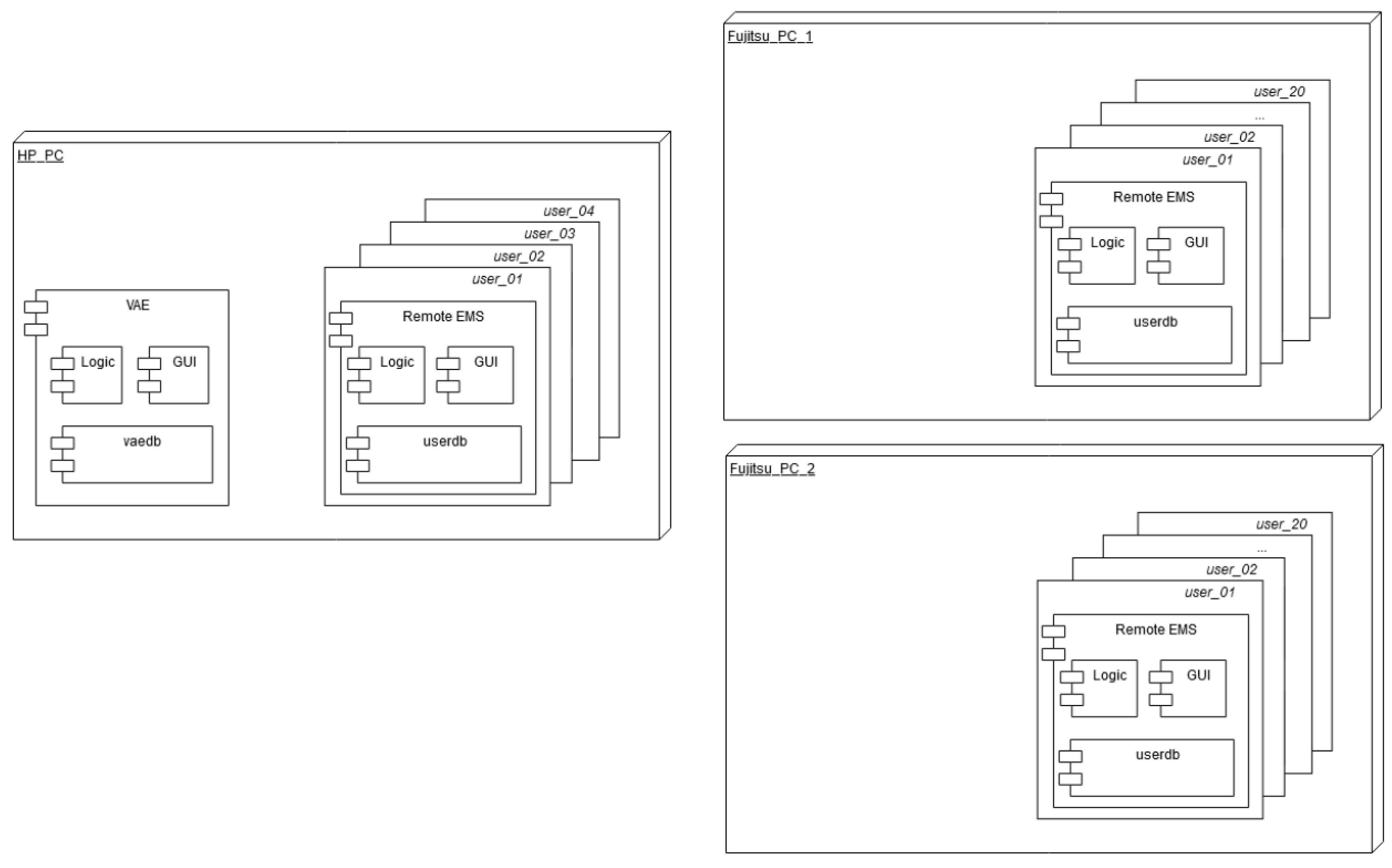
The VAE and the prosumers’ population is emulated using three computers with processor Intel CORE i5 7th generation: one PC with Windows 10 OS and 8 GB RAM for emulating the VAE and four prosumers (HP PC) and two PCs with Windows 7 OS and 4 GB RAM, for simulating other 40 prosumers (Fujitsu PC 1 and 2). The PCs need Java SE SDK v8.x, Tomcat v9.0.x, MySQL v8.0.x, Eclipse Mosquitto v1.6.x.
Figure 15 shows the deployment diagram of the test environment.
Various simulations were conducted to test the algorithm. Firstly, it was assumed that the DSO asks for a load reduction between 20,000 W and 75,000 W with a tolerance of ±1000 W to 44 residential and commercial prosumers. Since it is not possible that a single prosumer can satisfy the request from the DSO, the 44 prosumers start the aggregation policy in the VAE, creating aggregates able to totally or partially respond to the DSO request for a given price.
Various simulations were conducted to evaluate the time needed for the aggregation process. The results of the simulations are reported in
Figure 16, showing the elaboration time and the number of aggregates as a function of the required power variation. The results of the simulations show that, according to the algorithm operation described in
Section 3, the number of aggregates is between 1 and 7 and that the elaboration time for all the considered cases is between 20 and 29 min depending on the required power variation.
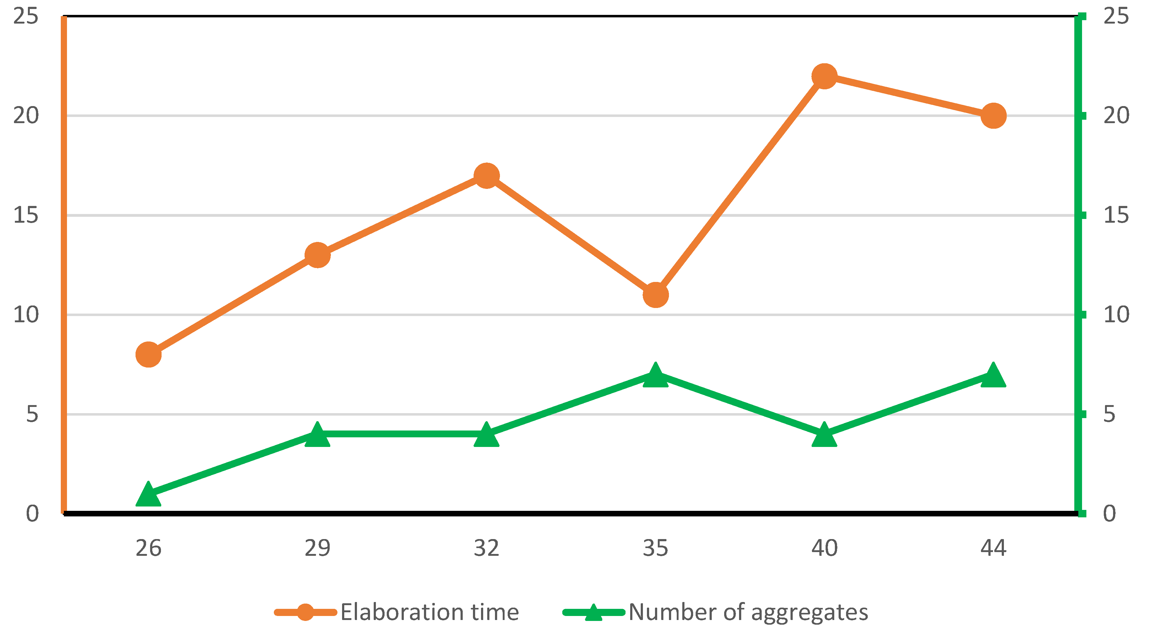
A second test was conducted by repeating the process of request and formulation of offers six times, keeping unchanged the variation in power required (20,000 W ± 1000 W) by varying the number of users involved in the process from time to time. The latter varied from a minimum of 26 to a maximum of 44. The elaboration time varies between 7 and 11 min in this case and is reported in
Figure 17.
In all examined cases, the elaboration time is compatible with the needs of the power systems. Indeed, since the aggregation process was performed the day before the need for flexibility, such elaboration times are acceptable and do not cause issues to the flexibility management.
Once the process has been completed, the VAE publishes in the “Offers Selection” page all the offers received, showing for each of them the total power variation in the aggregate, the requested price (including the surcharge due to the service provided by VAE), the overall reliability and score of the aggregate, an identification code of the offer and the number of aggregate users with the subdivision by type. The DSO is given the opportunity to select the offer it feels best suits its needs. Multiple criteria can be used to select the “best” bid, for example, selecting the bid with the lowest price/reliability ratio.
6. Conclusions
Alongside utility-scale BESS and other centralized solutions, DR and the aggregation of distributed resources is a very current research topic due to the need for power systems for solving the several issues caused by the unpredictability of RES and the increasing power peaks on lines and transformers.
Nevertheless, many commercial solutions for the management of distributed resources do not provide distributed logic enabling multi-stakeholder collaboration, mainly because these solutions are designed for users whose power consumption/generation levels are already sufficient to guarantee significant effects on the network. All smaller users are excluded from the flexibility market because they are unable to induce effects on the grid simply by exploiting their limited flexibility. The DEMAND project creates an architecture enabling prosumers of any kind (residential, commercial and industrial) to work together, aggregating them in a coordinated and intelligent way, without the need for centralized control.
The absence of a third-party aggregator allows simplifying the coordination issues and reducing the overall cost of the aggregation platform, allowing DSOs, TSOs and market operators to directly contact the end-users participating in the DEMAND project for exploiting their flexibility.
In this framework, the paper described two main algorithms developed for the bottom-up aggregation process in the framework of the DEMAND project. In the first part, the paper described the different phases for the management of the prosumer’s flexibility during the day-ahead operation and presented the algorithm for the management of this phase. In the second part, the algorithm for the bottom-up aggregation process and the selection of the winning offer were presented. The flexibility management algorithm allows for defining both the power variation offered by each end-user and the associated desired remuneration. Two case studies were presented considering a residential prosumer with and without PV and battery to show how the algorithm works. The two case studies show how the bids can be quite different depending on the devices that the prosumer can use for providing its flexibility and participating in the aggregation process, and on the classification of the end-user into “active” or “passive” categories defined by the Italian CEI Standard 0–21.
Finally, some considerations on the performance of the aggregation process in the VAE were shown for different power variations requested by the DSO and different sizes of the prosumers’ population. In all examined cases, the processing time was compatible with the scheduling needs of the DSO or a market participant.
The DEMAND project ended in July 2020 with the conclusion of the experimental phase on three pilots and with promising results. Some details on the pilots were reported in [
21]. In a future paper, the impact on the network of the aggregation process will be presented, together with the results of the cost-benefit analysis based on both the data collected from the pilots and the simulations performed considering the opportunities and threats of the emerging Italian flexibility market.


