A Method for Recognition of Sudden Commencements of Geomagnetic Storms Using Digital Differentiating Filters

Abstract

This article describes a method for recognizing sudden commencement events using digital differentiating filters. This method is applied to INTERMAGNET observatory data. Maximum amplitude derivatives for the magnetic components (X, Y, Z) and the total intensity (F) of the geomagnetic field are introduced, and the decision-making rule is formulated. The authors developed a procedure for selecting optimal digital differentiating filters. Estimates of probabilities of correct and false recognition of sudden commencements were obtained. The calculations of the probabilistic characteristics have confirmed the effectiveness of the method.

1. Introduction

The state of the Earth’s magnetosphere is monitored by INTERMAGNET observatories, which measure the components and total intensity of the geomagnetic field with a discrete-time sampling. Magnetic observatories are equipped with appropriate vector and scalar magnetometers and measure magnetograms in a given standard [1]. To date, there are 153 INTERMAGNET observatories in operation, located on all continents; INTERMAGNET magnetograms are hosted in a public database [2].

Geomagnetic disturbances arise due to the effects of plasma formations from solar coronal mass ejections on the Earth’s magnetosphere. A geomagnetic storm is generally an extreme phenomenon—a sporadic disturbance in the Earth’s magnetic field with high amplitudes (500–5000 nT). Sudden commencements (SC) of geomagnetic storms [3] are positive or negative jumps of the geomagnetic field, synchronously observed in almost all observatories. SC are a consequence of the impact of coronal mass ejecta on the Earth’s magnetosphere. Typical SC signals are the patterns characterized by an abrupt increase and decrease in the geomagnetic field intensity, which correspond to large values of derivatives. The duration of SC events ranges from minutes to tens of minutes, and the amplitudes of the jumps take on the values of units of percent from the mean level of the geomagnetic field intensity prior to SC; as a rule, SC are surrounded by noise-like geomagnetic field disturbances.

The main particularity of SC signals is in their occurrence prior to the moment of a geomagnetic storm onset. Calculating the estimates of SC signals as derivatives of the geomagnetic field is a completely natural approach to solving the problem of predicting the occurrence of a geomagnetic storm [3,4]. Reliable SC recognition is an urgent scientific and technical problem in the subject area of geomagnetism and solar–terrestrial physics.

A number of publications offer approaches to SC recognition with different efficiencies. For example, some publications [4,5,6] describe automated SC recognition techniques using Haar’s wavelets. In [7], it is recommended to use the actual SC characteristics, including amplitude, rise time, and maximum value of the derivative of SC signals. The authors in [8] describe the morphological elements of SC signals, on the basis of which the SC recognition system is built. In [9], the connection between SC events and space weather is discussed. The SC recognition method proposed in this study is aimed at supplementing the existing approaches. The proposed approach to solving the formulated problem of SC recognition consists of using differentiating filters for geomagnetic data. High-pass filtering using differentiating finite impulse response (FIR) filters is applied to clearly separate the SC signal. The structure of such filters is selected based on the problem of optimal use of data from a set of magnetic observatories for a certain time interval.

In Figure 1, an example of SC between 18:30 and 20:00 UTC is shown based on one-minute-averaged data of components $H_x$, $H_y,H_z$ and the total intensity $H_0$ of the geomagnetic field, registered at the ASP magnetic observatory (Alice Springs, Australia) on 22.06.2015 from 00:00 to 23:59. The 1440 values are in nT, $i=1,\dots ,N_0$, $N_0=1440$.

Similar geomagnetic field jumps followed by the mentioned increase in noise at 18:30–20:00 UTC were registered by all INTERMAGNET observatories.

2. Materials and Methods

2.1. Formulation of the SC Recognition Problem—Maximum Amplitude Derivatives and a Decision-Making Rule

Let us consider the variables $H_{xp}=H_{1p}$, $H_{yp}=H_{2p}$, $H_{zp}=H_{3p}$, and $H_{0p}$, which are the components and the total intensity of the geomagnetic field for a certain time interval where SC is present, obtained from a set of magnetic observatories, where p is the serial number of the magnetic observatory, and $p=1,\dots ,P_0$, $P_0$ is the total number of magnetic observatories. Further processing is based on the normalized records $H_{N,1p}\left(T\left(i\right)\right)$, $H_{N,2p}\left(T\left(i\right)\right)$, $H_{N,3p}\left(T\left(i\right)\right)$, and $H_{N,0p}\left(T\left(i\right)\right)$, obtained by subtracting the mean and normalizing the maximum amplitude of variations to ±1.

The SC recognition procedure for the normalized variables is based on three stages.

At the first stage, we estimate the first derivative of the discrete time series formed by the components of the geomagnetic field, which we denote as $H_{Nd,rp}^{\circ }\left(T\left(i\right)\right)$, r = 0, 1, … 3, $p=1,\dots ,P_0$ and obtained using the differentiating FIR filter (with a finite impulse-transient characteristic). We perform the differentiating FIR filtering using sliding averaging for normalized variables. First-order derivatives are calculated by discrete convolution of the normalized field record with a FIR filter of size $s_0$; that is,

$$H_{Nd,rp}^{\circ }\left(T\left(i\right)\right)={{\displaystyle \sum }}_{s=0}^{s_0}{a}_s{H}_{N,rp}\left(T\left(i-s\right)\right),$$

(1)

where $a_s$ are FIR filter weighting coefficients, $s=0,1,\dots ,s_0$, $s_0$ is the FIR filter size, $i=s_0+1,\dots ,N_f$, and $N_f$ is the time series length.

At the second stage, we calculate the maximum amplitude derivatives. To do this, we divide the initial time interval $i=1,\dots ,N_f$ into sub-intervals of constant length $\mathsf{\Delta }{i}_0$, limited by the boundary indices $[i_{1n},i_{2n}]$, $i_{1n}=1+\mathsf{\Delta }{i}_0\left(n-1\right)$, $i_{2n}=\mathsf{\Delta }{i}_{0}n$, and $n=1,\dots ,n_f$, where Δi₀ is also the sub-interval size, and $n_f$ is the total number of sub-intervals with $n_f\mathsf{\Delta }{i}_0=N_f$. For each sub-interval $n$, we calculate the absolute values of the derivatives $\left|H_{Nd,rp}^{\circ }\left(T\left(i\right),n\right)\right|$, $i_{1n}\le i \le i_{2n}$, $r=0,1\dots ,3$, and $p=1,\dots ,P_0$. Next, we find the maximum amplitude derivative,

$$H_{Nd}^{\circ } \left(n\right)=\underset{i_{1n}\le i\le i_{2n},r,p}{\max }\{|H_{Nd,rp}^{\circ }\left(T\left(i\right),n\right)|\},n=1,\dots ,n_f.$$

(2)

for each sub-interval and use these values for further analysis of the SC signal.

At the third stage, we perform the SC recognition by comparing the maximum amplitude derivatives $H_{Nd}^{\circ }\left(n\right)$, $n=1,\dots ,n_f$ with a predefined threshold $H_{Nd,0}^{}$. Let us assign a decision rule for recognition SC: if $H_{Nd}^{\circ }\left(n\right)\ge H_{Nd,0}$, then we decide that for the index $n$ there is SC, and if $H_{Nd} \left(n\right)<H_{Nd0}$, then we take the opposite decision.

2.2. The Procedure for Selecting the Optimal Digital Differentiating Filters

SC recognition depends on the type of FIR digital differentiating filter used (1). Optimal derivative estimates of a noisy discrete time series is always based on a compromise between accuracy, which involves the use of the shortest possible time interval, and noise suppression, which is based on the averaging effect obtained with discrete convolution over a certain number of samples. The selection of the mentioned FIR filters [10] will be performed based on the local approximation built on local intervals, the total number of which is $N_d$,

$$\begin{gathered} H_M\left(c_{rp},T\left(i\right)\right)={{\displaystyle \sum }}_{k=0}^{k_0}{c}_{rp,k}{(T\left(i\right))}^k,i,i-1,\dots ,i-N_d+1, \\ p=1,\dots ,P_0,r=0,1\dots ,3. \end{gathered}$$

(3)

of the signal with a polynomial of degree $k_0$, where the same polynomial coefficients $c_{rp,k}$ are used for each $T\left(i\right)$. The polynomial coefficients are thus found by minimizing the squared residuals,

$$S\left(H_{rp},H_M,i\right)={{\displaystyle \sum }}_{j=0}^{N_d-1}{(H_{rp}^{}\left(T\left(i-j\right)\right)-H_M\left(c_{rp},T\left(i-j\right)\right))}^2,$$

(4)

taken as the difference between the actual signal and its polynomial approximation. This is a linear problem whose solution yields the optimized coefficients $c_{rp,k }^{\circ }\left(i\right)$ for a given polynomial degree $k_0$ [10]. Once the optimal coefficients were calculated, the optimal derivative $H_{Nd,rp }^{\circ }\left(Ti\right)$ is calculated as follows:

$$H_{Nd,rp }^{\circ }\left(T\left(i\right)\right)={{\displaystyle \sum }}_{k=0}^{k_0}k{c}_{rp,k }^{\circ }\left(i\right)\cdot {(T(i))}^{k-1}.$$

(5)

The proposed optimization method is reliable enough because it is designed as a combination of the least squares method, which leads to solving the linear equation system, and the discrete sorting method.

2.3. Computation of Estimates of Probabilities of Correct and False SC Recognition

The optimal SC detection threshold is found by estimating the probabilities of correct and false SC recognition. Let us consider an approximate scheme for calculating the indicated probabilities.

Let us analyze a 1-year time series of 1-minute-sampled normalized data $H_{N,rp}\left(T\left(i\right)\right)$, $i=1,\dots ,N_f$ using the sub-intervals $[i_{1l},i_{2l}]$, with $i_{1l}=1+\mathsf{\Delta }{i}_0\left(l-1\right)$, $i_{2l}=\mathsf{\Delta }{i}_{0}l$, $l=1,\dots ,l_f$, and $l_f\mathsf{\Delta }{i}_0=N_f$. Next, we assume that $N_{SC}$ real SC events occurred within these $l_f\mathrm{intervals}$, and that $N_{RDSC }\le N_{SC}$ events have been identified with the method described above to be real. Let us assume that the number of local intervals for which there are no SC events is $N_{0SC}$ and the number of false recognitions turned out to be $N_{FDSC}$. Then,

$${\beta }_{RD}^{\circ }=N_{RDSC}/N_{SC},{\alpha }_{FD}^{\circ }=N_{FDSC}/N_{0SC}.$$

(6)

are the estimated probabilities for a correct and a false SC identification. Obviously the estimates of the probabilities ${\beta }_{RD }^{\circ }\left(H_{Nd,0}\right)$ and ${\alpha }_{FD}^{\circ }\left(H_{Nd,0}\right)$ (6) depend on the comparison threshold $H_{Nd,0}^{}$. The choice of the optimal threshold will be reduced to a conditional optimization problem. Let us introduce a limitation on the probability of false recognition ${\alpha }_0$ and set $H_{Nd,\alpha }^{}=\left\{H_{Nd,0}:\left(0\le {\alpha }_{FD}^{\circ }\left(H_{Nd,0}\right)\le {\alpha }_0\right)\right\}$ as the value for which the probability of false detection is $\le {\alpha }_{FD}^{\circ }$. The optimal threshold is thus given by the conditional optimization problem

$$H_{Nd,0}^{\circ }=\arg \left\{\underset{H_{Nd,0}\in H_{Nd,\alpha }}{\max }{\beta }_{RD}^{\circ }\left(H_{Nd,0}\right)\right\},$$

(7)

which can be solved iteratively. Let $H_{Nd,0mx}^{}{H}_{Nd,0mn}^{}$ be the maximum and minimum bounds of iterations within the maximum number of iteration steps $m_f$. Discrete threshold values are then defined as follows: $H_{Nd,0}^{}\left(m\right)=H_{Nd,0mn}^{}+\mathsf{\Delta }{H}_{Nd}^{}\left(m-1\right)$, $m=2,\dots ,m_f$, where the iteration step is $\mathsf{\Delta }{H}_{Nd}^{}=\left(H_{Nd,0mx }^{}-H_{Nd,0mn}^{}\right)/\left(m-1\right)$.

3. Results

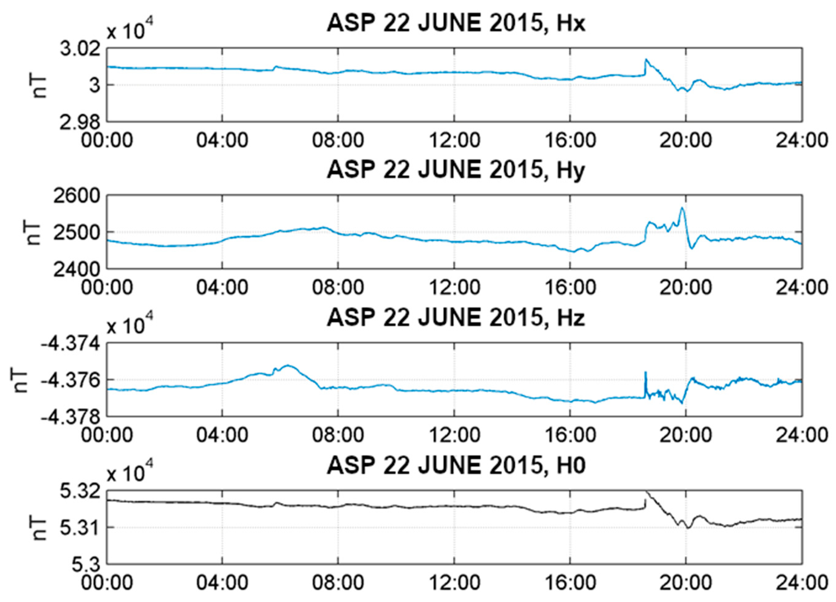
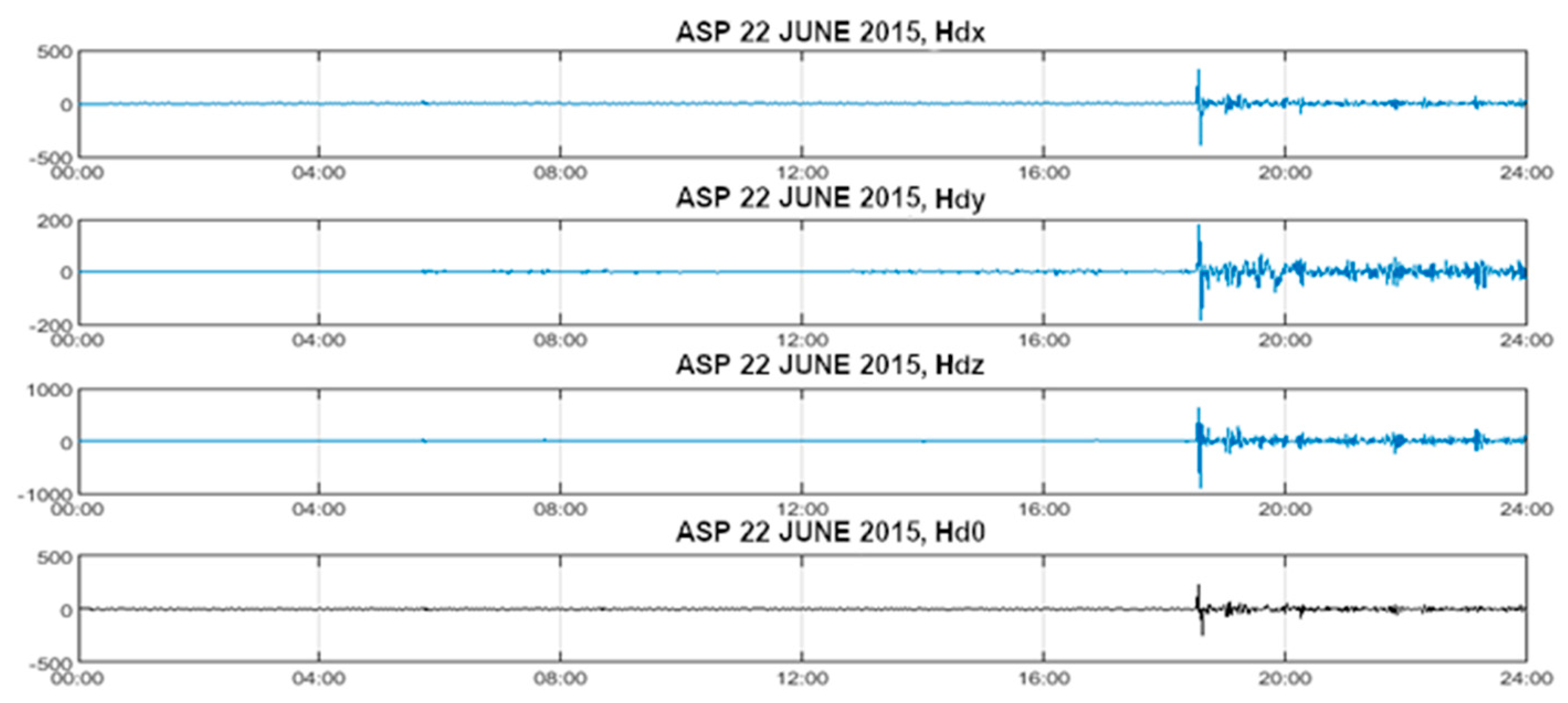
3.1. An Example of Optimal Differentiating FIR Filter Selection

We considered four types of FIR differentiating filters, labelled as m = 1, 2, 3, 4, for the calculation of the maximum amplitude derivative, according to Equation (5). These filters are characterized by $k_0$ (the filter order) and $i_d$ (the number of points used for approximation construction), which are assigned to the filter types as follows:

• $k_0$ = 1, $i_d$ = 2, for m = 1;
• $k_0$ = 1, $i_d$ = 3, for m = 2;
• $k_0$ = 2, $i_d$ = 4, for m = 3;
• $k_0$ = 3, $i_d$ = 5, for m = 4.

The ASP observatory and the daily data interval 22 June 2015 were chosen. For the sub-interval number $n=n_{SC}=111$, corresponding to the SC appearance time 18:35 UTC and the filter types m = 1, 2, 3, 4, we calculated the maximum amplitude derivatives of Equation (2) and determined the optimal filter type, which maximizes the maximum amplitude derivative

$$m^{\circ }=\arg \left\{\underset{m=1÷4}{\max }{H}_{Nd}^{\circ }\left(n_{SC},m\right)\right\}$$

(8)

and leads to the result $m^{\circ }=3$. The second-order differentiating filter with $k_0=2$ and $i_d=4$ min turned out to be the optimal one for the considered setting.

Figure 2 shows the results of calculating the derivatives for the components and the total intensity of the geomagnetic field using the second-order FIR filter $k_0=2$ and $i_d=4$, $r=0,1\dots ,3$, $p=1$, $H_{dx}=H_{Nd,11}^{}\left(T\left(i\right)\right),H_{dy}=H_{Nd,21}^{}\left(T\left(i\right)\right),H_{dz}=H_{Nd,31}^{}\left(T\left(i\right)\right),H_{d0}=H_{Nd,01}^{}\left(T\left(i\right)\right),i=1,2,\dots ,N_0$, and $N_0=1440$ ($T_{N_0}=24$ h).

The use of the optimized differentiating filter made it possible to reliably determine the beginning of the SC event. It can be seen that the SC event occurred in the interval with indices $i=1115÷1117$, corresponding to $\approx$18:35 UTC. In this interval, there was a sharp increase in the values of the derivatives for the components and the modulus, followed by noise components in the time interval $\approx$18:50–24:00 UTC.

The maximum amplitude derivatives for the field component and total field intensity were $\left|H_{Nd,11}^{\circ }\left(n_{SC},m\right)\right|=391$ nT/min, $\left|H_{Nd,21}^{\circ }\left(n_{SC},m\right)\right|=192$ nT/min, $\left|H_{Nd,31}^{\circ }\left(n_{SC},m\right)\right|=903$nT/min, and $\left|H_{Nd,-1}^{\circ }\left(n_{SC},m\right)\right|=245$ nT/min for $n_{SC}$= 111 and m = 4. At that the derivative turned out to be equal to $H_{Nd}^{\circ }\left(n\right)=903$ nT/min. Our analysis allows to conclude that the noise amplitude (about 48 to 60–70 nT/min) is 4–5 times less than the amplitudes of the maximum absolute derivatives.

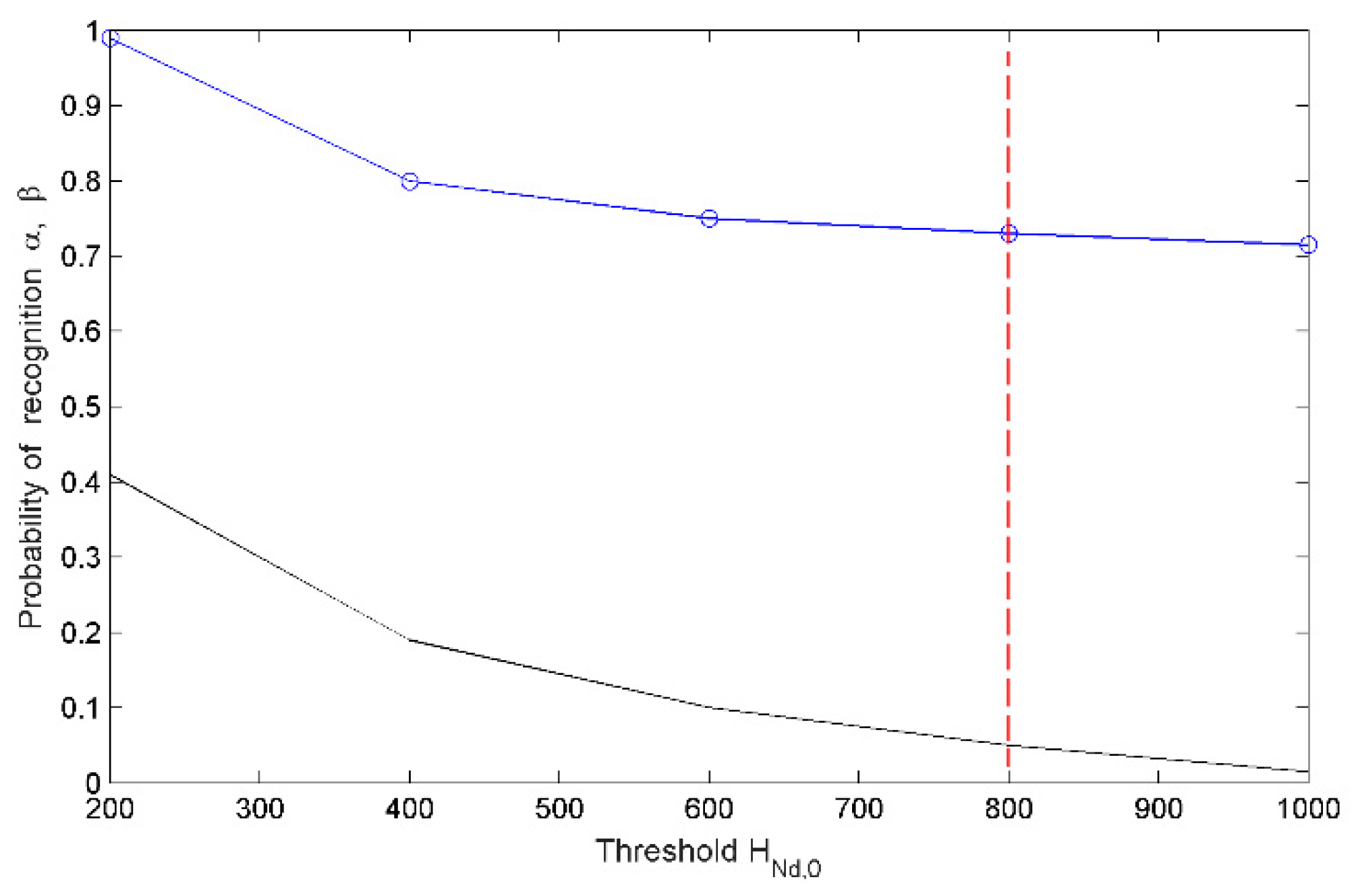
3.2. An Example of Estimates of Probabilities of True and False SC Recognitions

We used one-minute-averaged data from INTERMAGNET observatories [2]: ASP, BEL, BFO, BLC, BMT, BOU, BRW, BSL, CLF, CSY, CTA, DOU, EBR, ESK, EYR, and FCC. The total number of observatories in the calculation was $P_0=16$. We analyzed the 1-minute-sampled data for the whole period of 2015 $H_{rp}\left(T\left(i\right)\right)$, $r=0,1\dots ,3$, $p=1,\dots ,P_0$, $P_0=16$, comprising $T{N}_{f0}=T\cdot 1440\cdot 365=T\cdot 5.265\cdot {10}^5$ minutes. The local intervals $i_{1l},i_{2l}$, $i_{1l}=1+\mathsf{\Delta }{i}_0\left(l-1\right)$, $i_{2l}=\mathsf{\Delta }{i}_{0}l$, $l=1,\dots ,l_f$, $\mathsf{\Delta }{i}_0=10$ were determined; $l_f=5.265\cdot {10}^4$ is the number of local intervals.

A total of $N_{SC}$ = 17 global SC events were identified by the International Service on Rapid Magnetic Variations [11] at the INTERMAGNET observatory EBR (Ebro, Spain). The number of sub-intervals where SC were absent was $N_{0SC}=l_f-N_{SC}=5.2633\cdot {10}^4$.

For assigned iteration bounds $H_{Nd,0mx}^{}=1000$, $H_{Nd,0mn}^{}=200$, and $m_f=5$ a sequence of threshold values $H_{Nd,0}^{}\left(m\right)$ was calculated. Estimates of the probability of correct and false SC recognition were then obtained using Equation (6). Figure 3 shows the probabilities $\beta ={\beta }_{RD}^{\circ }\left(H_{Nd,0}\left(m\right)\right)$ and $\alpha ={\alpha }_{FD}^{\circ }\left(H_{Nd,0}\left(m\right)\right)$, as a function of the threshold value $H_{Nd,0}=H_{Nd,0}\left(m\right)$.

Our calculations show that if the probability of a false SC recognition is limited to ${\alpha }_0=0.05$, the optimal threshold value is $H_{Nd,0}^{\circ }\approx 800$ nT/min; in this case, the probability of correct SC recognition turned out to be ${\beta }_{RD}=$ 0.75. These probabilities indicate that our method for detecting SC events is quite effective. The method can be improved due to the optimal choice of the quantity of the analyzed datasets from magnetic observatories and increasing the temporal interval of observations.

4. Discussion

The proposed method for SC recognition on the basis of digital differentiating filters was tested using data from INTERMAGNET observatories for the year 2015.

The probability of correct detection of an SC event is ~75% when the probability of detecting a false event is limited to 5%. These results demonstrate the good performance of the proposed method.

The proposed SC recognition method has large possibilities for improvement, in particular, further optimization of the quantity of the analyzed datasets from magnetic observatories, as well as the temporal interval of the data analyzed in order to improve the probabilistic characteristics. The method can be adapted for solving the problem of short-term forecasting of a geomagnetic storm and has a favorable prospect for its use in applied problems.

In [4,5,6,7,8,9], solutions are given for various formulations of SC recognition problems. The main feature of the solutions presented is that observations from one observatory are used to obtain them. The proposed SC recognition here is based on a whole set of observatories. This approach is potentially more effective. The results supplement the studies of signals of natural origins based on approaches such as nonlinear adaptive filtering [12] or multifractal analysis [13].

References

1. St-Louis, B. Intermagnet Technical Reference Manual, version 4.6; Intermagnet: Edinburgh, UK, 2012; pp. 5–11. [Google Scholar]
2. Intermagnet. Available online: https://intermagnet.org/ (accessed on 3 November 2021).
3. Reay, S.J.; Herzog, D.C.; Alex, S.; Kharin, E.P.; McLean, S.; Nosé, M.; Sergeyeva, N.A. Magnetic Observatory Data and Metadata: Types and Availability. In Geomagnetic Observations and Models; Mandea, M., Korte, M., Eds.; Springer: Dordrecht, The Netherlands; Heidelberg, Germany; London, UK; New York, NY, USA, 2011; pp. 149–181. [Google Scholar]
4. Takano, S.; Minamoto, T.; Arimura, H.; Niijima, K.; Iyemori, T.; Araki, T. Automatic Detection of Geomagnetic Sudden Commencement Using Lifting Wavelet Filters. In Proceedings of the Second International Conference on Discovery Science (DS’99), Tokyo, Japan, 6–8 December 1999; Arikawa, S., Furukawa, K., Eds.; Springer: Berlin/Heidelberg, Germany, 1999; pp. 242–251. [Google Scholar]
5. Hafez, A.G.; Ghamry, E.; Yayama, H.; Yumoto, K. Wavelet Spectral Analysis Technique for Automatic Detection of Geomagnetic Sudden Commencements. IEEE Trans. Geosci. Remote Sens. 2012, 50, 4503–4512. [Google Scholar] [CrossRef]
6. Hafez, A.G.; Ghamry, E. Geomagnetic Sudden Commencement Automatic Detection via MODWT. IEEE Trans. Geosci. Remote Sens. 2013, 51, 1547–1554. [Google Scholar] [CrossRef]
7. Shinohara, M.; Kikuchi, T.; Nozaki, K. Automatic realtime detection of sudden commencements of geomagnetic storms. J. NICT 2005, 52, 197–205. [Google Scholar]
8. Satoru, T. Characteristics of geomagnetic sudden commencement observed in middle and low latitudes. Earth Planets Space 1998, 50, 735–772. [Google Scholar]
9. Space Weather Prediction Center, National Oceanic and Atmospheric Administration. Available online: https://www.swpc.noaa.gov (accessed on 29 October 2021).
10. Getmanov, V.G. Digital Signal Processing with Applications to Geophysics and Experimental Mechanics; Tekhnosfera: Moscow, Russia, 2021; pp. 61–71. (In Russian) [Google Scholar]
11. International Service on Rapid Magnetic Variations. Available online: http://www.obsebre.es/en/rapid (accessed on 1 November 2021).
12. Gao, J.B.; Hu, J.; Tung, W.W. Facilitating joint chaos and fractal analysis of biosignals through nonlinear adaptive filtering. PLoS ONE 2011, 6, e24331. [Google Scholar] [CrossRef] [PubMed] [Green Version]
13. Hu, J.; Gao, J.B.; Wang, X.S. Multifractal analysis of sunspot time series: The effects of the 11-year cycle and Fourier truncation. J. Stat. Mech. Theory Exp. 2009, 2, P02066. [Google Scholar] [CrossRef]
Figure 1. Plots of one-minute-averaged data of the components H x , H y ,   H z and the total intensity H 0 of the geomagnetic field strength vector with SC during 22 June 2015.
Applsci 12 00413 g001
Figure 2. Results of calculating the derivatives of the components and the modulus of the geomagnetic field (nT/min), ASP observatory.
Applsci 12 00413 g002
Figure 3. Estimated probability of correct (blue line with circles) and false (black line without circles) SC recognition. The red dashed line shows the optimal threshold value.
Applsci 12 00413 g003
Publisher’s Note: MDPI stays neutral with regard to jurisdictional claims in published maps and institutional affiliations.