
Prediction and Analysis of the Surface Roughness in CNC End Milling Using Neural Networks


Abstract
:1. Introduction
2. Prediction and Analysis of the Surface Roughness
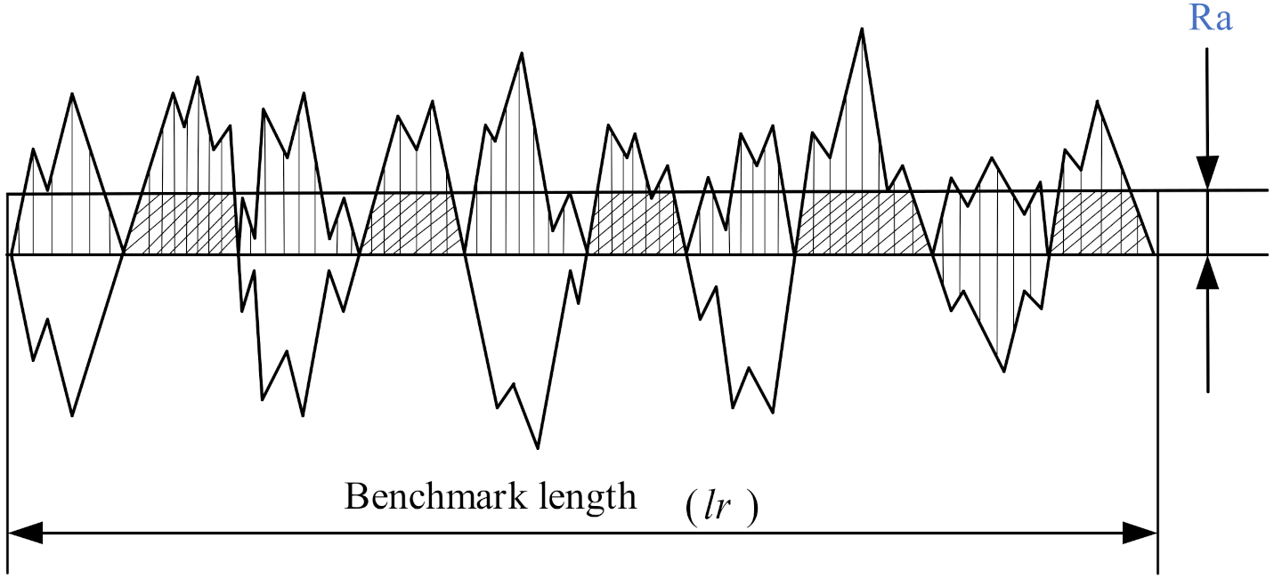
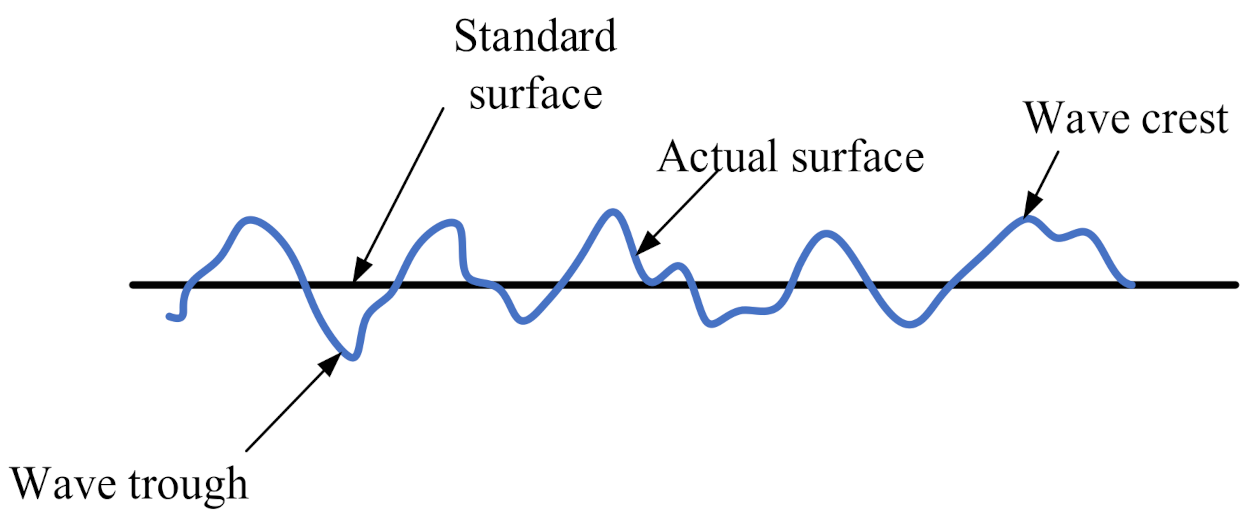
2.1. Surface Roughness and Experimental Setup
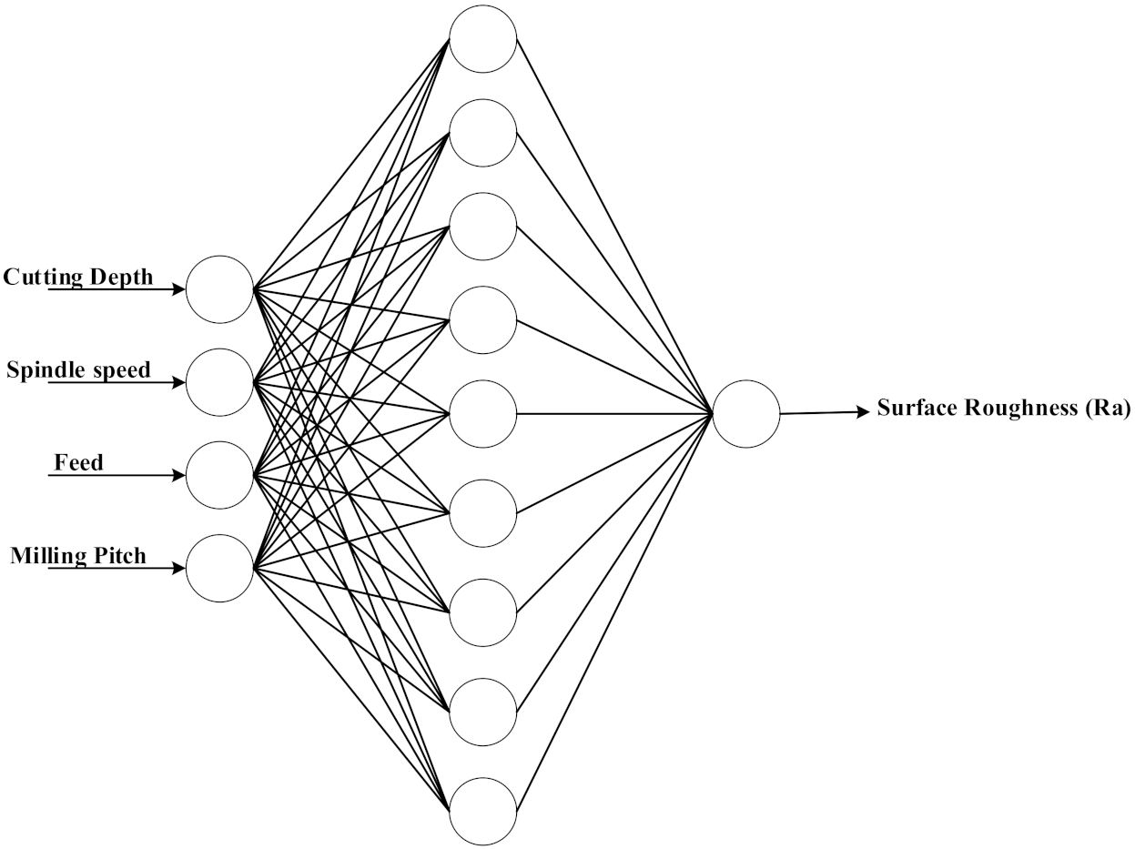
2.2. BPNN
2.3. Analysis of Variance
- The ethnic distributions implied by each group of samples must be normal or approximately normal.
- Each group of samples must be independent.
- The number of ethnic variations must be equal.
3. Results and Analysis
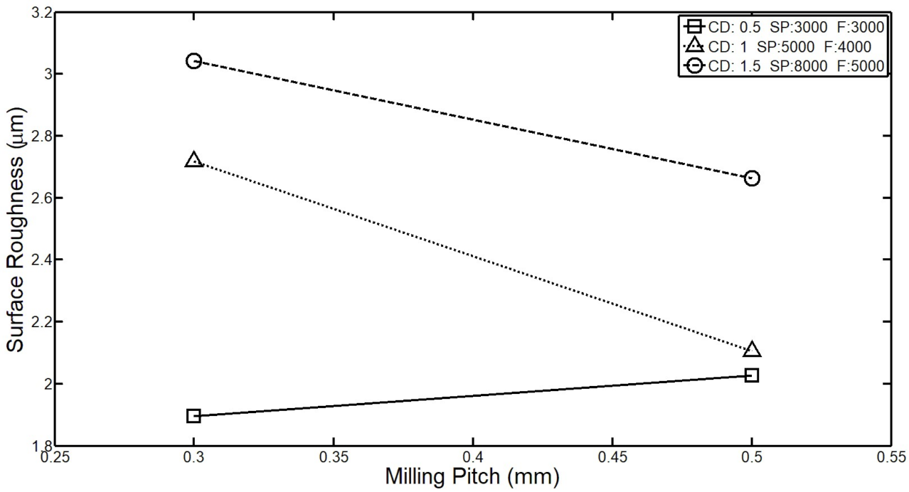
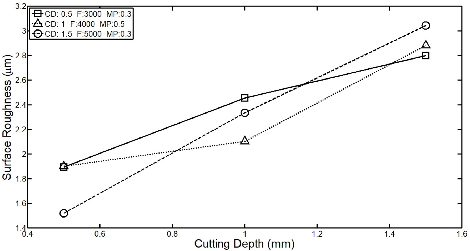
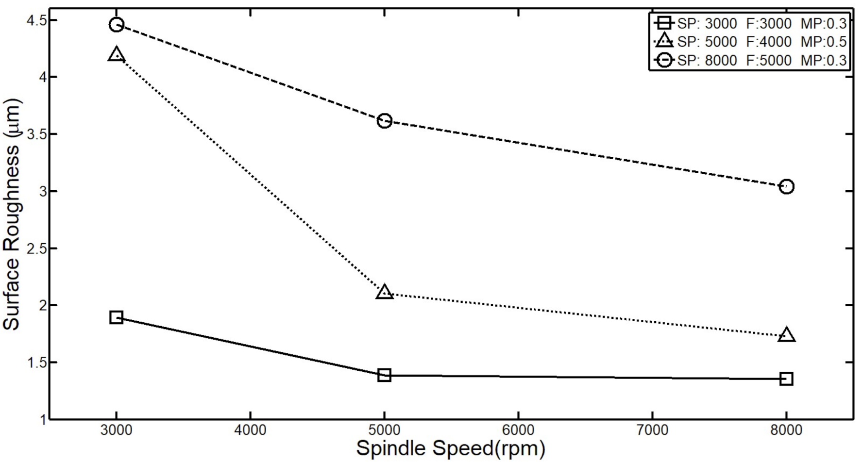
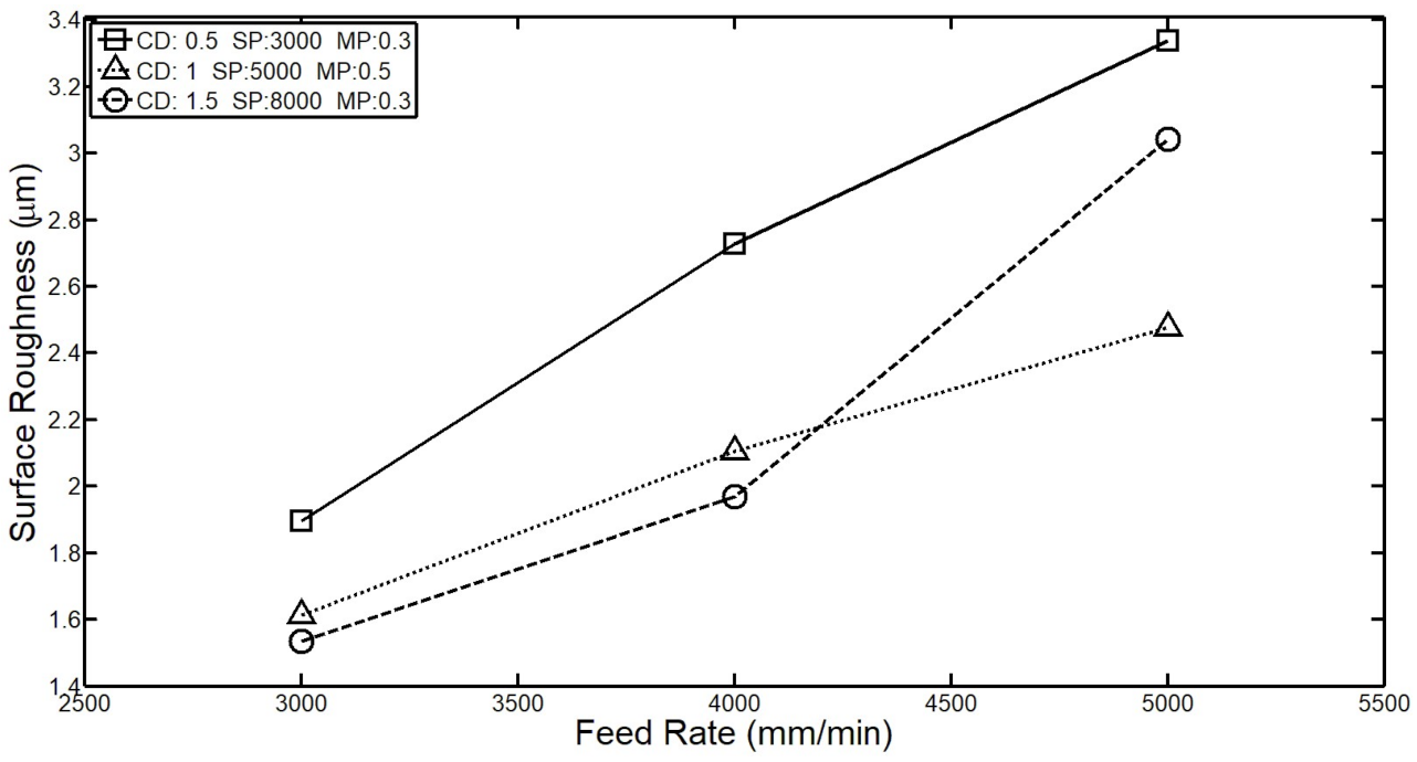
3.1. Effect of Input Parameters on Surface Roughness
3.2. Results of ANOVA
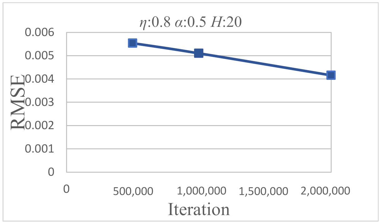
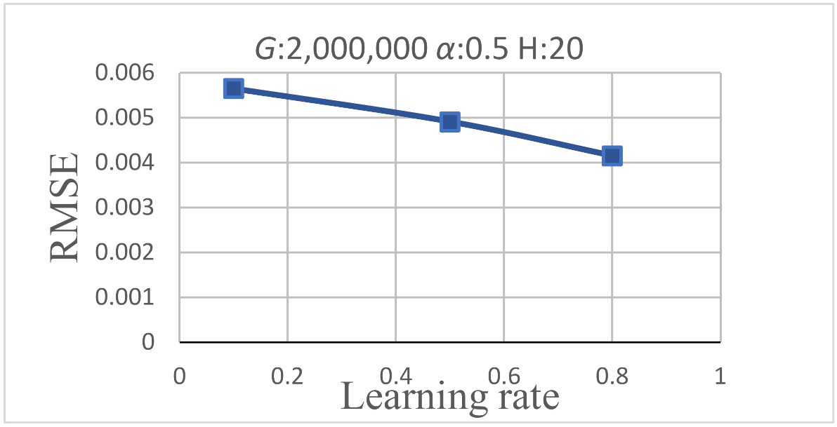
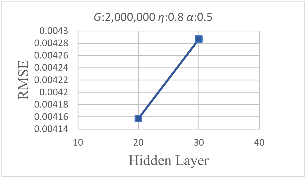
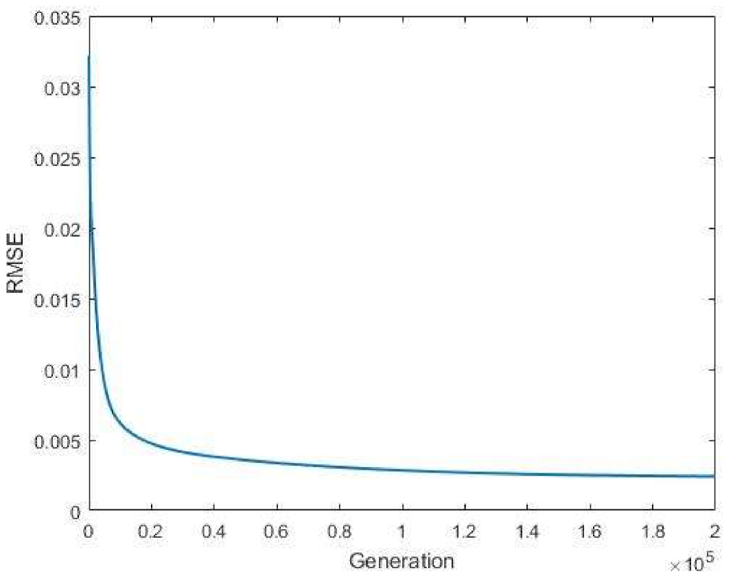
3.3. Parameter Analysis of BPNN
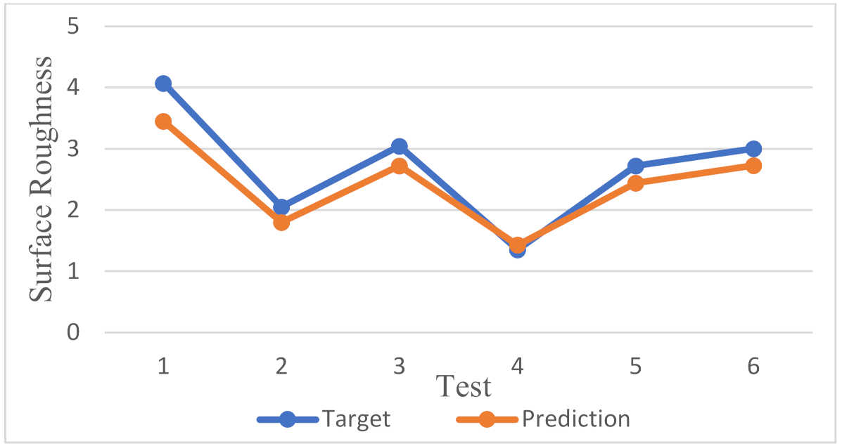
3.4. Predictive Results of BPNN
4. Conclusions
- (1)
- In the measurement experiment of surface roughness, the CNC parameters with a smaller cutting depth, a faster spindle speed, and a smaller feed rate will obtain a better surface roughness.
- (2)
- According to ANOVA, the contributions of the cutting depth, spindle speed, feed rate, and milling pitch in CNC were 51.86%, 77.48%, 92.3%, and 71%, respectively. This result shows that the feed rate has a greater influence on the surface roughness.
- (3)
- In the process of training neural networks, when the used BPNN with the number of iterations is set to 2,000,000, the learning rate is set to 0.8, the inertia factor is set to 0.5, and the number of hidden layer neurons is set to 20 it will have a lower RMSE.
- (4)
- In this study, linear regression and the used BPNN were compared. From the experimental results, it can be verified that the used BPNN has a lower RMSE and a higher . Furthermore, the prediction accuracy of linear regression and the used BPNN were 97.88% and 99.17%, respectively. According to the results, the used BPNN achieves excellent prediction of surface roughness.
Author Contributions
Funding
Institutional Review Board Statement
Informed Consent Statement
Data Availability Statement
Acknowledgments
Conflicts of Interest
References
- Kohli, A.; Dixit, U.S. A neural-network-based methodology for the prediction of surface roughness in a turning process. Int. J. Adv. Manuf. Technol. 2004, 25, 118–129. [Google Scholar] [CrossRef]
- Unune, D.R.; Mali, H.S. Artificial neural network–based and response surface methodology–based predictive models for material removal rate and surface roughness during electro-discharge diamond grinding of Inconel 718. Proc. Inst. Mech. Eng. Part B J. Eng. Manuf. 2016, 230, 2082–2091. [Google Scholar] [CrossRef]
- Sharma, V.S.; Dhiman, S.; Sehgal, R.; Sharma, S.K. Estimation of cutting forces and surface roughness for hard turning using neural networks. J. Intell. Manuf. 2008, 19, 473–483. [Google Scholar] [CrossRef]
- Tsao, C.C.; Hocheng, H. Evaluation of thrust force and surface roughness in drilling composite material using Taguchi analysis and neural network. J. Mater. Process. Technol. 2008, 203, 342–348. [Google Scholar] [CrossRef]
- Sanjay, C.; Jyothi, C. A study of surface roughness in drilling using mathematical analysis and neural networks. Int. J. Adv. Manuf. Technol. 2006, 29, 846–852. [Google Scholar] [CrossRef]
- Alagarsamy, S.V.; Ravichandran, M.; Meignanamoorthy, M.; Sakthivelu, S.; Dineshkumar, S. Prediction of surface roughness and tool wear in milling process on brass (C26130) alloy by Taguchi technique. Mater. Today Proc. 2020, 21, 189–193. [Google Scholar] [CrossRef]
- Benardos, P.G.; Vosniakos, G.C. Prediction of surface roughness in CNC face milling using neural networks and Taguchi’s design of experiments. Robot. Comput. Integr. Manuf. 2002, 18, 343–354. [Google Scholar] [CrossRef]
- Paturi, U.M.R.; Devarasetti, H.; Narala, S.K.R. Application of Regression and Artificial Neural Network Analysis In Modelling Of Surface Roughness In Hard Turning Of AISI 52100 Steel. Mater. Today Proc. 2018, 5, 4766–4777. [Google Scholar] [CrossRef]
- Markopoulos, A.P.; Manolakos, D.E.; Vaxevanidis, N.M. Artificial neural network models for the prediction of surface roughness in electrical discharge machining. J. Intell. Manuf. 2008, 19, 283–292. [Google Scholar] [CrossRef]
- Fredj, N.B.; Amamou, R. Ground surface roughness prediction based upon experimental design and neural network models. Int. J. Adv. Manuf. Technol. 2006, 31, 24–36. [Google Scholar] [CrossRef]
- Bagci, E.; Işık, B. Investigation of surface roughness in turning unidirectional GFRP composites by using RS methodology and ANN. Int. J. Adv. Manuf. Technol. 2006, 31, 10–17. [Google Scholar] [CrossRef]
- Ahmad, N.; Janahiraman, T.V.; Tarlochan, F. Modeling of Surface Roughness in Turning Operation Using Extreme Learning Machine. Arab. J. Sci. Eng. 2015, 40, 595–602. [Google Scholar] [CrossRef]
- Ezugwu, E.O.; Fadare, D.A.; Bonney, J.R.; Silva, B.D.; Sales, W.F. Modelling the correlation between cutting and process parameters in high-speed machining of Inconel 718 alloy using an artificial neural network. Int. J. Mach. Tools Manuf. 2005, 45, 1375–1385. [Google Scholar] [CrossRef]
- Karpat, Y.; Özel, T. Multi-objective optimization for turning processes using neural network modeling and dynamic-neighborhood particle swarm optimization. Int. J. Adv. Manuf. Technol. 2006, 35, 234–247. [Google Scholar] [CrossRef]
- Lee, S.S.; Chen, J.C. On-line surface roughness recognition system using artificial neural networks system in turning operations. Int. J. Adv. Manuf. Technol. 2003, 22, 498–509. [Google Scholar] [CrossRef]
- Karayel, D. Prediction and control of surface roughness in CNC lathe using artificial neural network. J. Mater. Processing Technol. 2009, 209, 3125–3137. [Google Scholar] [CrossRef]
- Mulay, A.; Ben, B.S.; Ismail, S.; Kocanda, A. Prediction of average surface roughness and formability in single point incremental forming using artificial neural network. Arch. Civ. Mech. Eng. 2019, 19, 1135–1149. [Google Scholar] [CrossRef]
- Zhong, Z.W.; Khoo, L.P.; Han, S.T. Prediction of surface roughness of turned surfaces using neural networks. Int. J. Adv. Manuf. Technol. 2005, 28, 688–693. [Google Scholar] [CrossRef]
- Dhokia, V.G.; Kumar, S.; Vichare, P.; Newman, S.T.; Allen, R.D. Surface roughness prediction model for CNC machining of polypropylene. Proc. Inst. Mech. Eng. Part B J. Eng. Manuf. 2008, 222, 137–157. [Google Scholar] [CrossRef]
- Sonar, D.K.; Dixit, U.S.; Ojha, D.K. The application of a radial basis function neural network for predicting the surface roughness in a turning process. Int. J. Adv. Manuf. Technol. 2005, 27, 661–666. [Google Scholar] [CrossRef]
- Zerti, A.; Yallese, M.A.; Zerti, O.; Nouioua, M.; Khettabi, R. Prediction of Mechanical Engineers. Part C J. Mech. Eng. Sci. 2019, 233, 4439–4462. [Google Scholar] [CrossRef]
- Thangarasu, S.S.; Mohanraj, T.; Devendran, K. Tool wear prediction in hard turning of EN8 steel using cutting force and surface roughness with artificial neural network. Proc. Inst. Mech. Eng. Part C J. Mech. Eng. Sci. 2019, 234, 329–342. [Google Scholar]


| Blade Diameter (d) | Blade Length (L1) | Tool Length (L) | Number of Edges (F) | Helix Angle |
|---|---|---|---|---|
| 10 (mm) | 30 (mm) | 75 (mm) | 3 | 45° |
| Spindle Speed | Feed | ||
|---|---|---|---|
| 5760 (rpm) | 1260 (mm/min) | 1.5 (mm) | 0.1 (mm) |
| 1 Layer | 2 Layer | 3 Layer | |
|---|---|---|---|
| Feed (mm/min) | 3000 | 4000 | 5000 |
| Spindle speed(rpm) | 3000 | 5000 | 8000 |
| Cutting depth (mm) | 0.5 | 1 | 1.5 |
| Milling pitch (mm) | 3 | 5 |
| Item | Parameter |
|---|---|
| Workbench size (mm) | 320 |
| Maximum workpiece rotation diameter (mm) | 400 |
| Maximum workpiece size (mm) | 400 × 300 |
| Workbench load (kg) | 100 |
| X-axis (mm) | 410 |
| Y-axis (mm) | 610 |
| Z-axis (mm) | 510 |
| A-axis | +30°~120° |
| C-axis | 360° |
| Maximum spindle speed (rpm) | 10,000 |
| Controller | SIEMENS |
| No. | Cutting Depth (mm) | Spindle Speed (rpm) | Feed (mm/min) | Milling Pitch (mm) | Ra () |
|---|---|---|---|---|---|
| 1 | 0.5 | 3000 | 3000 | 0.3 | 1.895 |
| 2 | 0.5 | 3000 | 4000 | 0.3 | 2.729 |
| 3 | 0.5 | 3000 | 5000 | 0.3 | 3.337 |
| 4 | 0.5 | 3000 | 3000 | 0.5 | 2.027 |
| 5 | 0.5 | 3000 | 4000 | 0.5 | 2.700 |
| 6 | 0.5 | 3000 | 5000 | 0.5 | 3.487 |
| 7 | 0.5 | 5000 | 3000 | 0.3 | 1.386 |
| 8 | 0.5 | 5000 | 4000 | 0.3 | 1.517 |
| 9 | 0.5 | 5000 | 5000 | 0.3 | 1.645 |
| 10 | 0.5 | 5000 | 3000 | 0.5 | 1.416 |
| 11 | 0.5 | 5000 | 4000 | 0.5 | 1.903 |
| 12 | 0.5 | 5000 | 5000 | 0.5 | 2.249 |
| 13 | 0.5 | 8000 | 3000 | 0.3 | 1.354 |
| 14 | 0.5 | 8000 | 4000 | 0.3 | 1.377 |
| 15 | 0.5 | 8000 | 5000 | 0.3 | 1.520 |
| 16 | 0.5 | 8000 | 3000 | 0.5 | 1.523 |
| 17 | 0.5 | 8000 | 4000 | 0.5 | 1.425 |
| 18 | 0.5 | 8000 | 5000 | 0.5 | 1.439 |
| 19 | 1 | 3000 | 3000 | 0.3 | 2.455 |
| 20 | 1 | 3000 | 4000 | 0.3 | 2.959 |
| 21 | 1 | 3000 | 5000 | 0.3 | 4.070 |
| 22 | 1 | 3000 | 3000 | 0.5 | 3.378 |
| 23 | 1 | 3000 | 4000 | 0.5 | 4.191 |
| 24 | 1 | 3000 | 5000 | 0.5 | 3.721 |
| 25 | 1 | 5000 | 3000 | 0.3 | 2.221 |
| 26 | 1 | 5000 | 4000 | 0.3 | 2.717 |
| 27 | 1 | 5000 | 5000 | 0.3 | 2.483 |
| 28 | 1 | 5000 | 3000 | 0.5 | 1.612 |
| 29 | 1 | 5000 | 4000 | 0.5 | 2.105 |
| 30 | 1 | 5000 | 5000 | 0.5 | 2.476 |
| 31 | 1 | 8000 | 3000 | 0.3 | 1.683 |
| 32 | 1 | 8000 | 4000 | 0.3 | 2.049 |
| 33 | 1 | 8000 | 5000 | 0.3 | 2.336 |
| 34 | 1 | 8000 | 3000 | 0.5 | 1.395 |
| 35 | 1 | 8000 | 4000 | 0.5 | 1.731 |
| 36 | 1 | 8000 | 5000 | 0.5 | 2.069 |
| 37 | 1.5 | 3000 | 3000 | 0.3 | 2.801 |
| 38 | 1.5 | 3000 | 4000 | 0.3 | 3.813 |
| 39 | 1.5 | 3000 | 5000 | 0.3 | 4.461 |
| 40 | 1.5 | 3000 | 3000 | 0.5 | 3.018 |
| 41 | 1.5 | 3000 | 4000 | 0.5 | 5.509 |
| 42 | 1.5 | 3000 | 5000 | 0.5 | 23.901 |
| 43 | 1.5 | 5000 | 3000 | 0.3 | 3.005 |
| 44 | 1.5 | 5000 | 4000 | 0.3 | 2.838 |
| 45 | 1.5 | 5000 | 5000 | 0.3 | 3.617 |
| 46 | 1.5 | 5000 | 3000 | 0.5 | 2.722 |
| 47 | 1.5 | 5000 | 4000 | 0.5 | 2.883 |
| 48 | 1.5 | 5000 | 5000 | 0.5 | 3.586 |
| 49 | 1.5 | 8000 | 3000 | 0.3 | 1.534 |
| 50 | 1.5 | 8000 | 4000 | 0.3 | 1.969 |
| 51 | 1.5 | 8000 | 5000 | 0.3 | 3.043 |
| 52 | 1.5 | 8000 | 3000 | 0.5 | 1.312 |
| 53 | 1.5 | 8000 | 4000 | 0.5 | 2.469 |
| 54 | 1.5 | 8000 | 5000 | 0.5 | 2.663 |
| Sum of Square (SS) | Degree of Freedom (DF) | Mean of Square (MS) | F (Test) | p-Value | |
|---|---|---|---|---|---|
| Between group | (Group-1) | Table search | |||
| Within group | |||||
| Total | (Samples-1) |
| SS | DF | MS | F | p-Value | Critical Value | Con (%) | |
|---|---|---|---|---|---|---|---|
| 59.3598 | 1 | 59.3598 | 112.0691 | <0.0001 | 3.932438 | 51.86% | |
| 55.08584 | 104 | 0.529672 | |||||
| 114.4456 | 105 |
| SS | DF | MS | F | p-Value | Critical Value | Con (%) | |
|---|---|---|---|---|---|---|---|
| 7.66 × 10⁸ | 1 | 7.66 × 10⁸ | 357.9129 | <0.0001 | 3.932438 | 77.48% | |
| 2.22 × 10⁸ | 104 | 2,138,970 | |||||
| 9.88 × 10⁸ | 105 |
| SS | DF | MS | F | p-Value | Critical Value | Con (%) | |
|---|---|---|---|---|---|---|---|
| 4.19 × 10⁸ | 1 | 4.19 × 10⁸ | 1247.14 | <0.0001 | 3.932438 | 92.3% | |
| 3.49 × 10⁷ | 104 | 336,357.5 | |||||
| 4.54 × 10⁸ | 105 |
| SS | DF | MS | F | p-Value | Critical Value | Con (%) | |
|---|---|---|---|---|---|---|---|
| 115.6564 | 1 | 115.6564 | 256.6285 | <0.0001 | 3.932438 | 71% | |
| 46.87036 | 104 | 0.450677 | |||||
| 162.5268 | 105 |
| 500,000 | 1,000,000 | 2,000,000 | |
| 0.1 | 0.5 | 0.8 | |
| 0.5 | 0.8 | ||
| 20 | 30 |
| No. | RMSE | ||||
|---|---|---|---|---|---|
| 1 | 500,000 | 0.1 | 0.5 | 20 | 0.006509797 |
| 2 | 500,000 | 0.1 | 0.5 | 30 | 0.006452063 |
| 3 | 500,000 | 0.1 | 0.8 | 20 | 0.006119852 |
| 4 | 500,000 | 0.1 | 0.8 | 30 | 0.006391917 |
| 5 | 500,000 | 0.5 | 0.5 | 20 | 0.005824562 |
| 6 | 500,000 | 0.5 | 0.5 | 30 | 0.005207749 |
| 7 | 500,000 | 0.5 | 0.8 | 20 | 0.005122899 |
| 8 | 500,000 | 0.5 | 0.8 | 30 | 0.005292113 |
| 9 | 500,000 | 0.8 | 0.5 | 20 | 0.005538547 |
| 10 | 500,000 | 0.8 | 0.5 | 30 | 0.005474869 |
| 11 | 500,000 | 0.8 | 0.8 | 20 | 0.005046593 |
| 12 | 500,000 | 0.8 | 0.8 | 30 | 0.00503299 |
| 13 | 1,000,000 | 0.1 | 0.5 | 20 | 0.006459028 |
| 14 | 1,000,000 | 0.1 | 0.5 | 30 | 0.006260511 |
| 15 | 1,000,000 | 0.1 | 0.8 | 20 | 0.00545881 |
| 16 | 1,000,000 | 0.1 | 0.8 | 30 | 0.005549763 |
| 17 | 1,000,000 | 0.5 | 0.5 | 20 | 0.005418789 |
| 18 | 1,000,000 | 0.5 | 0.5 | 30 | 0.005435733 |
| 19 | 1,000,000 | 0.5 | 0.8 | 20 | 0.004799067 |
| 20 | 1,000,000 | 0.5 | 0.8 | 30 | 0.004720272 |
| 21 | 1,000,000 | 0.8 | 0.5 | 20 | 0.005104896 |
| 22 | 1,000,000 | 0.8 | 0.5 | 30 | 0.005057594 |
| 23 | 1,000,000 | 0.8 | 0.8 | 20 | 0.004475259 |
| 24 | 1,000,000 | 0.8 | 0.8 | 30 | 0.004706842 |
| 25 | 2,000,000 | 0.1 | 0.5 | 20 | 0.005654144 |
| 26 | 2,000,000 | 0.1 | 0.5 | 30 | 0.005682413 |
| 27 | 2,000,000 | 0.1 | 0.8 | 20 | 0.005117443 |
| 28 | 2,000,000 | 0.1 | 0.8 | 30 | 0.005167562 |
| 29 | 2,000,000 | 0.5 | 0.5 | 20 | 0.004917882 |
| 30 | 2,000,000 | 0.5 | 0.5 | 30 | 0.004883775 |
| 31 | 2,000,000 | 0.5 | 0.8 | 20 | 0.00446712 |
| 32 | 2,000,000 | 0.5 | 0.8 | 30 | 0.004655432 |
| 33 | 2,000,000 | 0.8 | 0.5 | 20 | 0.004157405 |
| 34 | 2,000,000 | 0.8 | 0.5 | 30 | 0.004286702 |
| 35 | 2,000,000 | 0.8 | 0.8 | 20 | 0.00504091 |
| 36 | 2,000,000 | 0.8 | 0.8 | 30 | 0.00500624 |
| Model | RMSE | |
|---|---|---|
| Linear regression | 0.021215796 | 0.7794 |
| BPNN | 0.008338854 | 0.9995 |
Publisher’s Note: MDPI stays neutral with regard to jurisdictional claims in published maps and institutional affiliations. |
© 2021 by the authors. Licensee MDPI, Basel, Switzerland. This article is an open access article distributed under the terms and conditions of the Creative Commons Attribution (CC BY) license (https://creativecommons.org/licenses/by/4.0/).
Share and Cite
Chen, C.-H.; Jeng, S.-Y.; Lin, C.-J. Prediction and Analysis of the Surface Roughness in CNC End Milling Using Neural Networks. Appl. Sci. 2022, 12, 393. https://doi.org/10.3390/app12010393
Chen C-H, Jeng S-Y, Lin C-J. Prediction and Analysis of the Surface Roughness in CNC End Milling Using Neural Networks. Applied Sciences. 2022; 12(1):393. https://doi.org/10.3390/app12010393
Chicago/Turabian StyleChen, Cheng-Hung, Shiou-Yun Jeng, and Cheng-Jian Lin. 2022. "Prediction and Analysis of the Surface Roughness in CNC End Milling Using Neural Networks" Applied Sciences 12, no. 1: 393. https://doi.org/10.3390/app12010393
APA StyleChen, C.-H., Jeng, S.-Y., & Lin, C.-J. (2022). Prediction and Analysis of the Surface Roughness in CNC End Milling Using Neural Networks. Applied Sciences, 12(1), 393. https://doi.org/10.3390/app12010393