CAIT: A Predictive Tool for Supporting the Book Market Operation Using Social Networks

Abstract

A new predictive support tool for the publishing industry is presented in this note. It consists of a combined model of Artificial Intelligence techniques (CAIT) that seeks the most optimal prediction of the number of book copies, finding out which is the best segmentation of the book market, using data from the networks social and the web. Predicted sales appear to be more accurate, applying machine learning techniques such as clustering (in this specific case, KMeans) rather than using current publishing industry expert’s segmentation. This identification has important implications for the publishing sector since the forecast will adjust more to the behavior of the stakeholders than to the skills or knowledge acquired by the experts, which is a certain way that may not be sufficient and/or variable throughout the period.

1. Introduction

When a book is launched, the publisher faces a big problem: how many books should be printed? This is known in the industry as print runs. Books that are not sold in stores are returned to the warehouse. Naturally, publishers do not want returns, nor do they want books that languish in the warehouse. For the publisher, this implies increased cost of promotion, correction time, legal procedures, etc.; for the environment, this leads to higher impact due to paper consumption to procedure surplus copies of the book. For example, during 2018, up to 40% of the 225 million titles published in Spain were returned [1].

Currently, the publishing industry uses the knowledge of marketing experts as a predictive measure, classifying sales (or the number of copies to print) into four fundamental segments. This classification is not using, however, the information coming from social networks and internet searches and mentions. As Fishbein and Azjen [2] wrote, “the best individual predictor of an individual’s behavior will be a measure of his intention to perform that behavior”. Since social network analysis can provide and insight on the market pulse, we are driven to pose the following research question: Will the identification of the market segments of the book using the stakeholders’ behavior in social networks and the web improve the prediction of copies to print?

In this way, the main objectives that we set ourselves with this research are:

• Find a better segmentation method.
• Adjust the prediction of copies to print to each segment found.
• Create a combined model of Artificial Intelligence techniques (CAIT), which will serve as a support tool to predict the number of books copies contributes to increasing revenue (publishers only).

Starting from the base of our research question and the objectives set, we hypothesize that an automatic segmentation can predict and/or improve current results with the experts’ segmentation.

The article is organized as follows. First, in Section 2, we review the work related to the topic that we will propose to work on. Then, Section 3, we will describe our research design depicting the data and the method used. Next, the experimentation results are presented in Section 4. Finally, in Section 5, we discuss our results and conclude by describing the general contributions of the research, the ethical aspects of being mindful of the use of Artificial Intelligence, as well as future directions.

2. Background

The estimation of the number of copies to be printed of a new book is at present determined by the editor’s experience and ability to gauge the potential reader’s interest. In order to assess the viability of a decision support tool, relying on information of social networks and internet mentions, let us review first three key aspects such as (a) The influence of social networks on sales, (b) The success of a book based on sales, and (c) Sales segmentation forecast techniques.

2.1. The Influence of Social Networks on Sales

From the perspective of social influence, no study in the publishing sector considers the impact of social networks on the product. Still, there are many similar cases in different retail industries. Fashion, for example, ref. [3], shows us that a strong presence in social networks is important for the sale of a product, rather than being under the advertising standards by the industry; mobile telephony [4], they indicate us how these communication channels can be used to predict the income of a product or entertainment [5], reveal that beyond social networks, valuable information can be extracted from famous blogs. Specifically, this paper [6] proposes to use the number of blog references as an indicator of the success of the sale of a book. Another work [7] understands the effects of social networks in the interactions of the seller and the consumer, offering us new insights on how social influence improves the impacts of consumption and contributes positively to the performance of the retailers and consumer loyalty. Following this line of thought, we found another study [8] based on the customer’s commitment to a product or brand, which reinforces the importance that this feature may have for future predictions. Recent publications such as [9] serve as the basis to begin to understand the mechanics of reader preference. Still, they are only based on the sale of bestsellers, thus leaving a large gap in the sale of the remaining books. Another article like [10] makes us reflect on the effect that sharing the famous “likes” of consumers on social networks has on sales, exerting great social pressure in the community.

2.2. The Success of a Book Based on Sales

From the point of view of the success of the book based on sales, we reference this work [11] which analyzes the characteristics that make a book a bestseller, using statistical techniques and data analysis. However, the work is aimed exclusively at authors already recognized by readers. Another study [12] is only based on historical book sales data and some attributes collected from Amazon. Up to this point of the investigation, none of the sources includes social networks in the publishing sector to predict sales. Still, they help us consider which characteristics to input for the prediction model.

2.3. Sales Segmentation Forecast Techniques

The goal of segmentation is to partition heterogeneous groups into homogeneous subgroups based on similarities. One of the most widely used statistical techniques for this purpose is quartiles [13], which divide populations into four groups, or quarters, of equal size. The following work [14] allows us to analyze the use of quartiles for market segmentation, but it is only focused on the purchaser. The consumer market in this paper is segmented by price, where it is shown that wealthy purchasers pay moderately higher prices for pills and injectables. Another study [15] reveals a negative wage gap in the lowest quartile from the wage distribution of an employment balance in Russia. These articles are useful, as they provide us with a segmentation technique that we will use to compare with the expert’s segmentation (currently used) in the publishing sector. Finally, although following this line of research, revising state of the art, these works [16,17,18] where pattern matching techniques are applied to time series data are interesting because they use the similarity of historical data as a basis for grouping time series. All this allows us to visualize an idea of grouping the historical information of the books, but we still need to incorporate the data from social networks and the web.

Finally, no study considers the impact of the presence of social networks in the prediction of the number of copies to print of a book (or what is the same sales) and, especially, that it is done automatically.

3. Research Design and Method

This section describes the proposal of a new decision support tool to help publishers determine the number of copies to print. Using as a basis three methods of segmentation of the book market: (1) a priori segmentation based on quartiles, the most basic proposal, (2) segmentation based on the criteria of experts, current segmentation, and (3) grouping the data according to their behavior patterns, automatic segmentation.

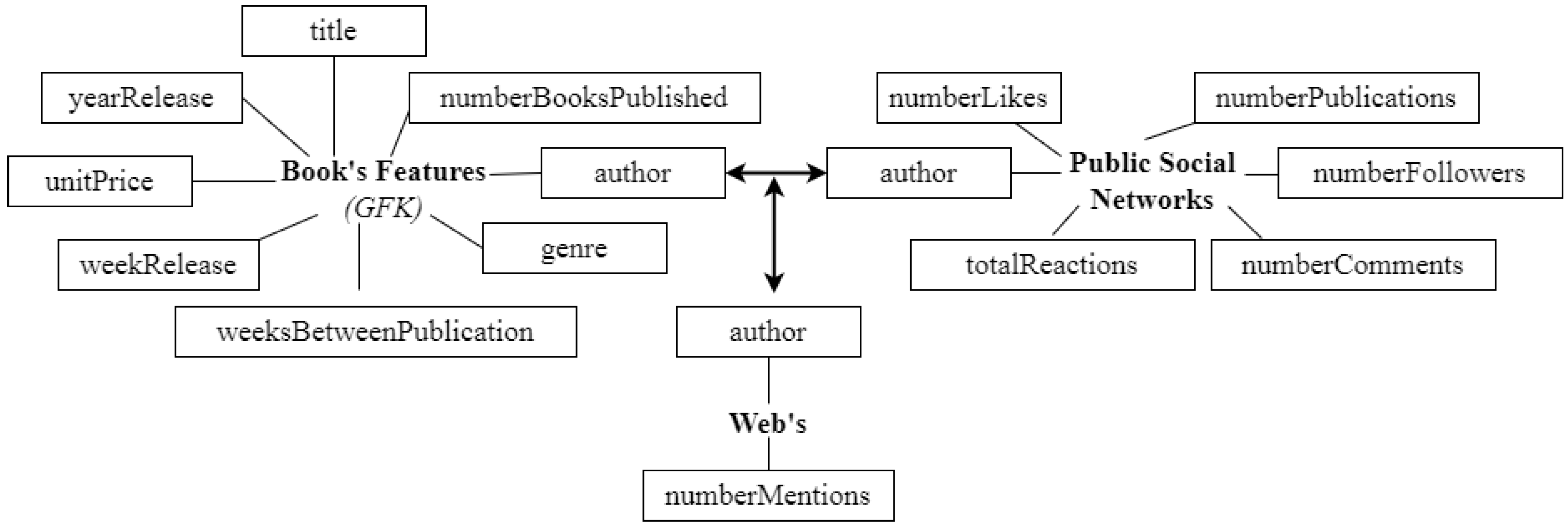
3.1. Description of the Dataset

The data used is provided by (from now on, we will call it) “The Editorial”, respecting the anonymity of the medium; and correspond to the data of GFK [19] on the sale of books. It contains book titles, authors, release dates, price, and other features. The data is limited to the territory of Spain during the 2018–2020 period and to the literary genres Non-Fiction and Children/Youth. As a sample, 1169 books have been used, which, according to the experts of the publishing industry, are considered more sensitive to the popularity of the author. The analysis is based on the characteristics of a book, the author’s public social networks, and web mentions, which are shown in Figure 1.

For a better understanding of the experimentation that we will carry out in Section 4, in Figure 2 we will observe the three different segmentations that we can perform on the data. After obtaining the classification label to test whether our hypothesis is true or false, we pass the new data through a combined classification and regression model to determine the precise number of copies for each segmentation.

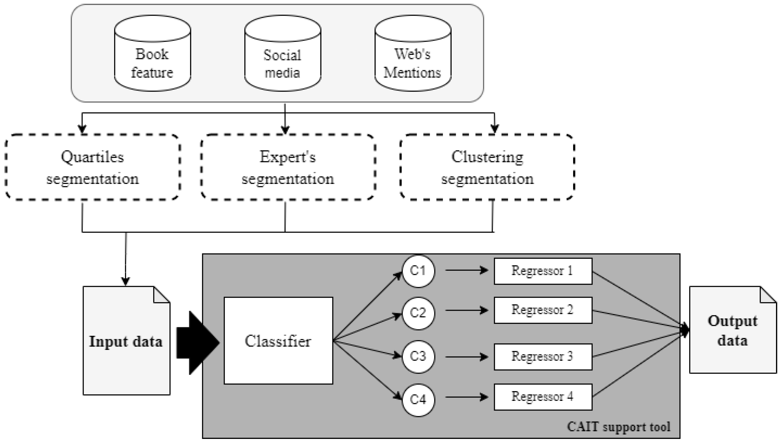
3.2. CAIT: The Proposal

Once we have the input data, it contains the characteristics of the book, the data from social networks, the number of mentions on the Web, and the segmentation according to the book market. Then, they are entered into the support tool to verify the accuracy of the predictions. In this subsection, we will present the composition of the CAIT and the considerations that were considered for the selection of the optimal algorithm in the two parts of this combined model, according to the processed data. The use of classifiers (Part A) is due to the previously performed segmentation, based on the objective variable (number of copies or, what is the same, book sales). This analysis will be detailed in Section 4 and the use of regressors (Part B) because, thanks to its linear adjustment, it can bring us closer to the dependency relationship between the independent and dependent variables. Next, we will describe each of its components and, finally, the proposed predictive support system.

3.2.1. Part A: The Classifier

Three classification algorithm shall be considered for the implementation of the classifier. These are,

• Decision Tree: It is a representation in the form of a tree whose branches branch according to the values taken by the variables and which end in a specific action. It is generally used when the number of conditions is not very large in this study. See [20,21] for a detailed description of this algorithm.
• Random Forest: It is a combination of predictor trees such that each tree depends on the values of a random vector tested independently and with the same distribution for each of these. It is implemented in data mining to classify or forecast a target variable. See [22,23] for a detailed description of this algorithm.
• K-Nearest Neighbors: It is a classification method used to estimate the density function of the predictors for each class. See [24,25] for a detailed description of this algorithm.
• XGBoost: Part of the decision tree that is implemented in data mining to classify or forecast on a target variable (book copies), through machine learning that is performed on a set of data, using several weak classifiers. In this case, they are the decision trees, but enhancing the results of these, due to the sequential processing of the data with a loss or cost function, minimizes the error iteration after iteration, thus making it a strong predictor. However, this will depend on the level of adjustment of the parameters used in the function. See [26,27] for a detailed description of this algorithm.

For our specific dataset, as will be detailed in Section 4, the best algorithm is XGBoost. We can observe the implementation of this algorithm in Algorithm 1, in which we will enter the input data that is made up of the characteristics of the book, the author’s social media data, plus the mentions it has on the web ($X_i$). Finally, the output is given by the different segmentations into which books can be divided based on the number of copies of a book ($Y_i$).

Algorithm 1 Classifier phase

Split:$D_{total}$ in $D_{train}$ and $D_{test}$ (from K-Fold stratified cross-validation, in this case k = 10) Input:$D_{train}$ = ($X_j$, $Y_j$) Where the target variable will be the segmentation   1: An initial tree $F_0$ is obtained to predict the objective variable $Y_j$, the residual is associated with the difference ($Y_j-F_0$).   2: A new tree “$h_1$” is obtained that adjusts the error to the previous weight.   3: The results of $F_0$ and $h_1$ are combined to obtain the tree $F_1$, where the mean square error of $F_1$ will be less than that of $F_0$   4:   $F_{1}x<-F_{0}x+h_1\left(x\right)$   5: This process is continued iteratively until the error is minimized as much as possible in the following way:   6:   $F_{m}x<-F_m-1x+h_m\left(x\right)$   7: The classifier is tested with $D_{test}$ using Accuracy, Precision, Recall, F1Score, and MAE as the evaluation metrics. Output:$Y_{class}$, predicted segmentation.

3.2.2. Part B: The Regressors

In the second part, we use the regressor algorithms; with them, the aim is to study the effect of one or more independent variables on a single dependent variable. The dependent variable (Y) will be the one we seek to survey through statistical regression to understand how it adapts when modifying the independent variables ($X_i$). After mathematically describing what has just been explained, we can obtain the following formula:

$$Y=0+B_1\ast X_1+B_2\ast X_2+\dots +B_n\ast X_n+\epsilon$$

(1)

where Y represents the dependent variable that is being studied or trying to predict, $X_1,X_2...X_n$ are all the independent variables that influence or can affect the dependent variable Y. The function of $\epsilon$ is to explain the possible variability of the data that cannot be presented through the linear relationship of the formula; in other words, it represents the possible existing error.

Knowing the objective and operation of the regressor algorithms, we show below those selected for the competition, looking for the one that best suits the input data:

• Gradient Boosting: It is a machine learning technique [28,29] which produces a predictive model in the form of a set of weak prediction models (typically decision trees). When building the model, it is done in a stepwise manner (as boosting methods do), and it generalizes them, allowing the arbitrary optimization of a differentiable loss function.
• XGBoost: Described in previous section.
• LightGBM: It is a distributed gradient impulse framework for machine learning. It is based on decision tree algorithms but does not grow at the tree level but in leaves. Therefore, by choosing the one will produce the greatest decrease in loss. See [30] for a detailed description of this algorithm.

For our specific dataset, as will be detailed in Section 4, the best algorithm is XGBoost. The implementation of this algorithm can be observed in Algorithm 2, in which we will enter as input data the characteristics of the book, the author’s social network data, plus the mentions that this has on the web ($X_j$). The output is our objective variable that will be given by the number of copies ($Y_j$).

Algorithm 2 Regressor phase

Split:$D_{total}$ in $D_{train}$ and $D_{test}$ (from K-Fold stratified cross-validation, in this case k = 10) Input:$D_{train}$ = ($X_j$, $Y_j$) Where the target variable will be the number of copies   1: An initial tree $F_0$ is obtained to predict the objective variable $Y_j$, the residual is associated with the difference ($Y_j-F_0$).   2: A new tree “$h_1$” is obtained that adjusts the error to the previous weight.   3: The results of $F_0$ and $h_1$ are combined to obtain the tree $F_1$, where the mean square error of $F_1$ will be less than that of $F_0$   4:   $F_{1}x<-F_{0}x+h_1\left(x\right)$   5: This process is continued iteratively until the error is minimized as much as possible in the following way:   6:   $F_{m}x<-F_m-1x+h_m\left(x\right)$   7: The regressor is tested with $D_{test}$ using $R^2$ as the evaluation metric. Output:$Y_{predicted}$, predicted number of copies.

3.2.3. CAIT: A Predictive Support Tool

Once we have described each component of our proposed predictive support tool, we can observe in the Algorithm 3 its implementation, where we introduce the characteristics of the book, the author’s social network, web mentions, and the segmentation of said data ($X_k$). These data will go through the classification function, obtaining as a result which segmentation group each book can belong to. Given this classification, the data corresponding to each group will be divided, and the regressors will be applied individually through hyperparameters optimization. The details of the hyperparameters used can be seen in Section 4.

Algorithm 3 CAIT algorithm

Input:$X_k$   1: class = Classifier phase ($X_k$)   2: if class == 1:   3:   Regressor phase ($X_k$)   4: elseif class == 2:   5:   Regressor phase ($X_k$)   6: elseif class == 3:   7:   Regressor phase ($X_k$)   8: elseif class == 4:   9:   Regressor phase ($X_k$) Output:$Y_{nbcopies}$, number of book copies to print according to its segmentation in the market.

Finally, this subsection has detailed the composition of the predictive support tool created. Demonstrating the effect of obtaining its best advantages from each part and joining them in one helps us improve the precision of the number of copies.

4. Results

This section shows the different distributions that a priori data can have with one of the segmentations to be evaluated. First, the most basic segmentation is carried out, quartiles; then expert segmentation is used, and finally, automatic segmentation is given by pattern matching. Subsequently, each of them is tested in the support tool, showing the comparison results of each of the parts referred to in Section 3, seeking the improvement of the predictions. All calculations were performed in Python [31] on Intel (R) Core™ i5-9400F @ 2.90GHz PC CPU.

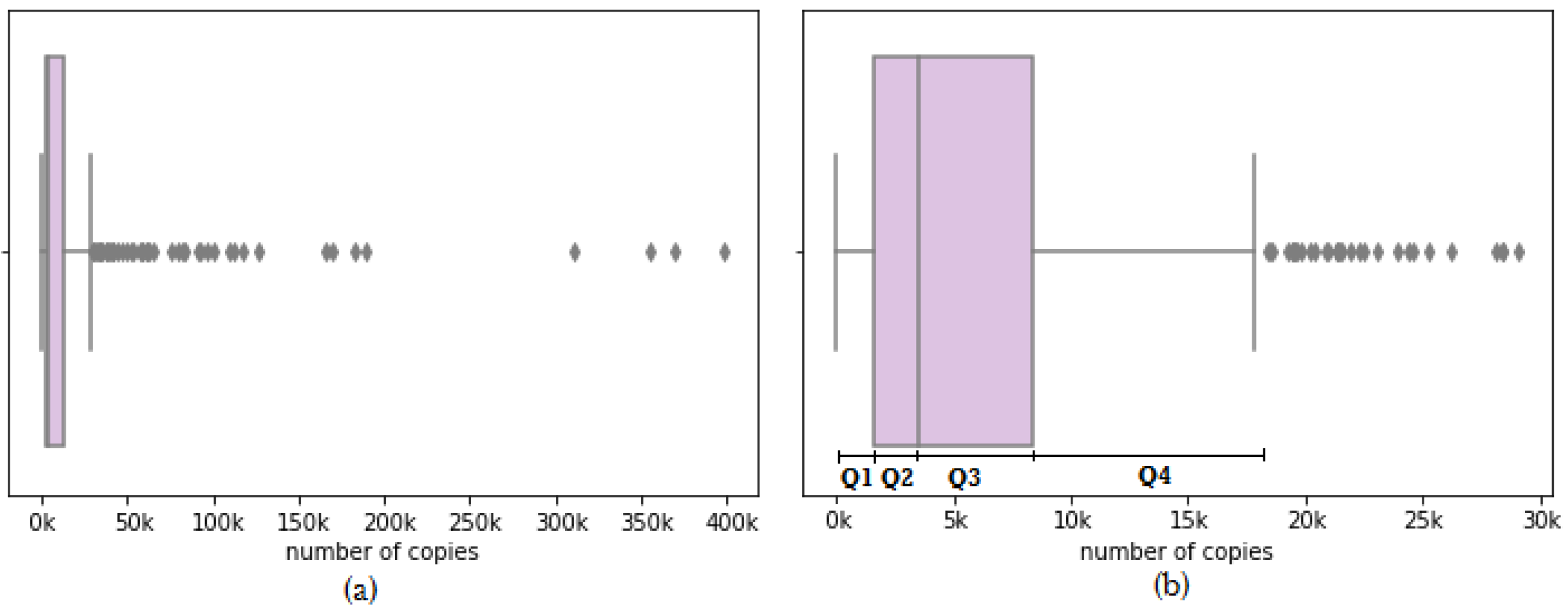
4.1. Quartiles Segmentation (the Most Basic Segmentation)

The first segmentation to test is the quartiles. Quartiles have been selected influenced by the segmentation of the experts after the analysis of the project requirement. For the dataset used, the numbers of book copies are grouped by author. If we observe Figure 3a, we can detect the existence of outliers, and they are eliminated above 1.5 of the interquartile range. Finally, we are left with Figure 3b, in which we can easily identify the 4 quartiles into which the number of copies can be segmented, being: less than 1808 (Q1—low sales); between 1808 and 4229 (Q2—low intermediate sales); between 4229 and 12 781 (Q3—high intermediate sales); and finally greater than 12781 (Q4—high sales) copies. This last quartile is the so-called Bestseller books. We will refer to the quartiles as classes so that it is easier later to compare them with the rest of the segmentations to be analyzed. A better understanding of the distribution of volume of data by the different segmentations of the quartiles can be seen in Figure 4.

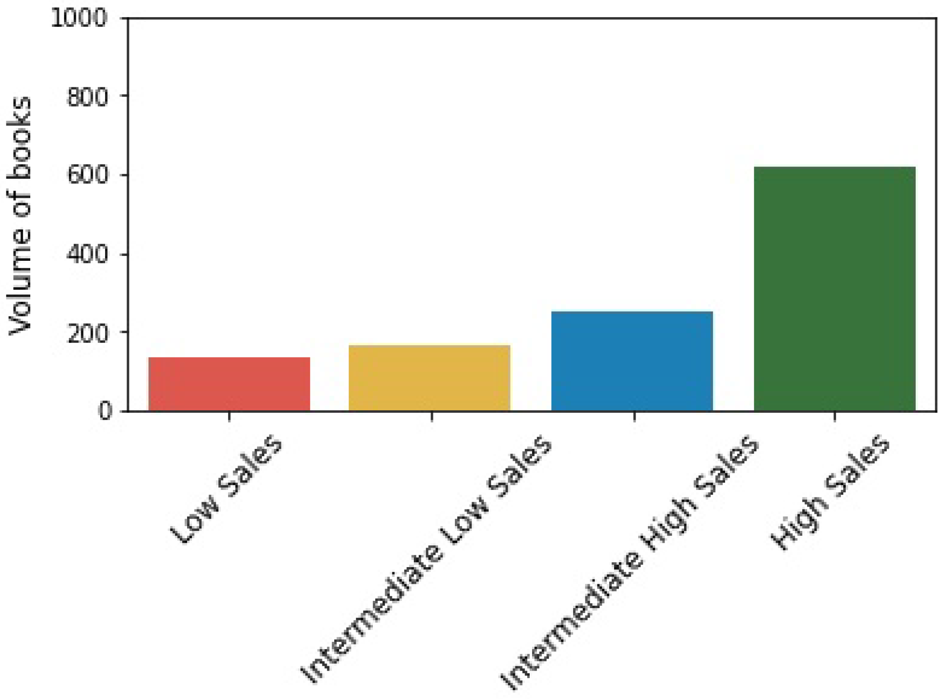
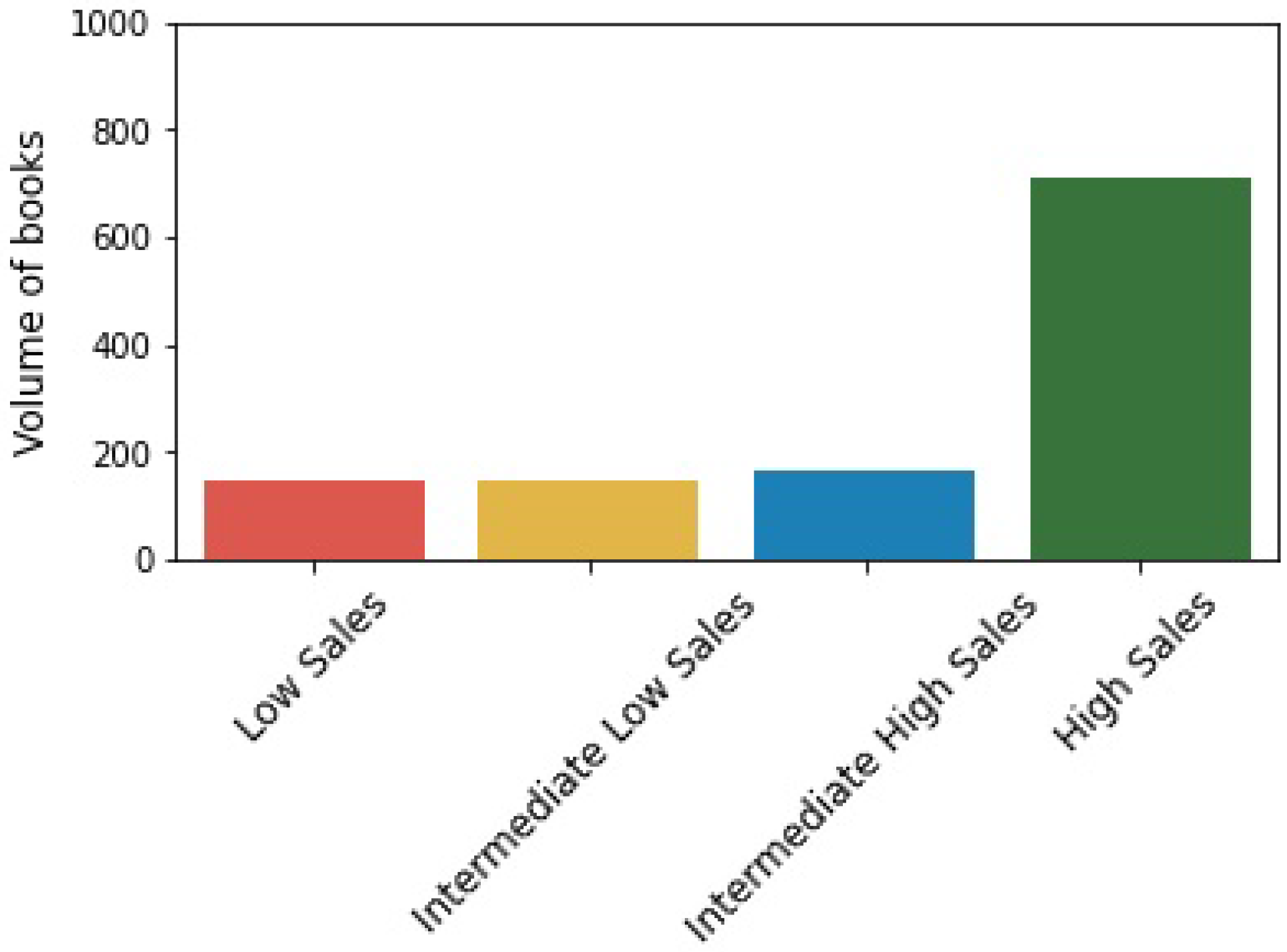
4.2. Expert’s Segmentation (the Current Segmentation)

The experts provide the segmentations after the analysis of the project requirement. They will be identified as class 1—low sales (C1), class 2—low intermediate sales (C2), class 3—high intermediate sales (C3), and class 4—high sales (C4). The reason for the segmentation carried out by the experts will not be detailed, but in Figure 5 the volume of data due to the different segmentations will be observed.

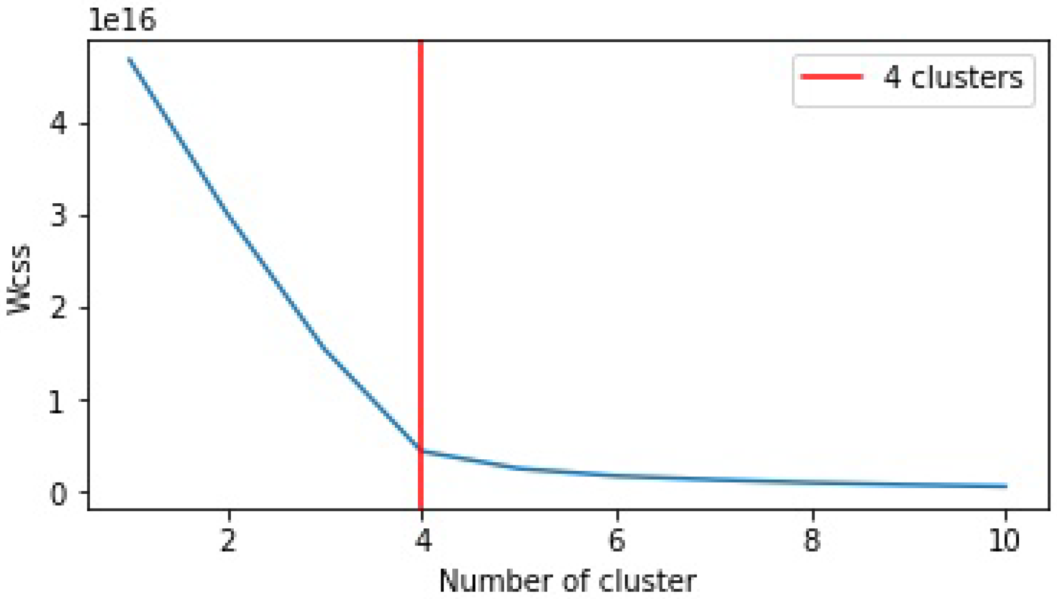
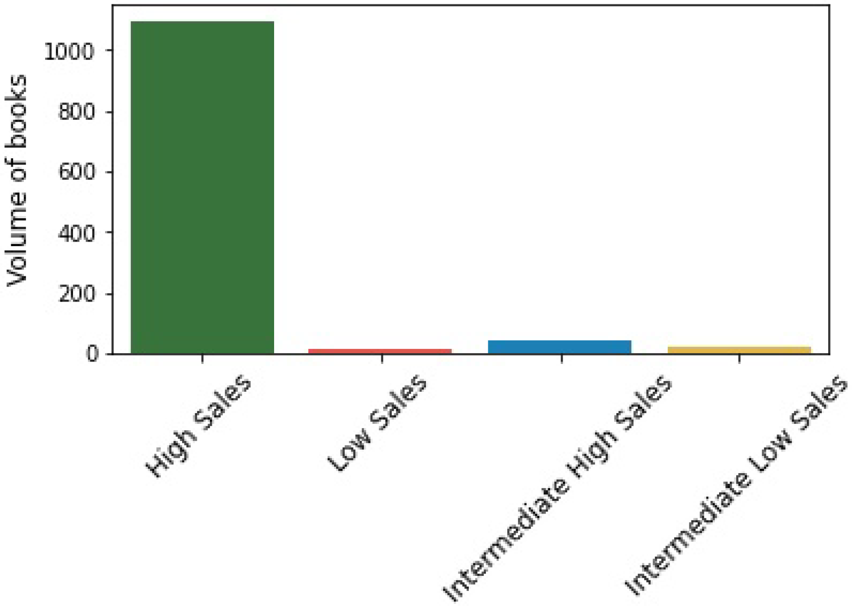
4.3. Clustering (the Automatic Segmentation)

Before applying unsupervised learnings techniques for pattern matching, it is necessary to establish the optimal number of k groups. For this, we use the Elbow curve, which consists of plotting the sum of squared distance between each point and the centroid in a cluster (Wcss). As the number of clusters increases, the Wcss value will decrease. The rule applied to choose $k=4$, as we can see in Figure 6. These results confirm that the number of segments suggested by the experts from the start is correct but that they can be obtained regardless of their knowledge.

Once we have selected the optimal number of clusters to group our data based on their behavior, we use the K-means, the simplest and fastest training method. In Figure 7 we can see the volume of data presented by the 4 clusters detected by KMeans. They will be identified as class 1—low sales (C1), class 2—low intermediate sales (C2), class 3—high intermediate sales (C3), and class 4—high sales (C4).

If we analyze Figure 4, Figure 5 and Figure 7, some of the classes have a fairly low volume. Therefore, before using any prediction method such as the one we will use with the predictive support tool CAIT, the data is balanced.

4.4. Performance Evaluation Methods: For Classification Part

• K-Fold stratified cross-validation, this validation seeks to ensure that each k group is representative in all data strata. It is intended to ensure that each class is (roughly represented equally in each test fold) and thus avoid overtraining. In this specific case, our variable k = 10
• Accuracy (Equation (2)), which refers to how close a sample statistic is to a population parameter, being TP (true positive value), TN (true negative value), FP (false positive value), FN (false negative value).
• Precision (Equation (3)) with which this algorithm hits each of the classes is also analyzed.
• Recall (Equation (4)), represents the model’s ability to correctly predict the positives out of actual positives.
• F1-Score (Equation (5)), this gives a weighted average of the precision and recall metrics. It is the best metric for averaging out and balancing all the evaluation metrics as a whole.
• Mean Absolute Error (MAE) is used, which is a measure of the difference between two continuous variables (Equation (6)). Where $y_i$ is the prediction, $\widehat{y}$ and the true value.

$$Accuracy=\frac{TP+TN}{TP+TN+FP+FN}$$

(2)

$$Precision=\frac{TP}{TP+FP}$$

(3)

$$Recall=\frac{TP}{TP+FN}$$

(4)

$$F1-Score=\frac{Precision\ast Recall}{Precision+Recall}$$

(5)

$$MAE(y,\widehat{y})=\frac{1}{n_{samples}}\sum _{i=0}^{n_{samples}}|y_i-{\widehat{y}}_i|$$

(6)

Algorithm Comparison Analysis

All the values of the metrics discussed above are combined into a single overall scorecard for each classifier for each of the segmentations.

As can be observed in

Table 1. Comparison of classifiers algorithms with quartiles segmentation. This table shows that the XGBoost algorithm is the optimal one of the four to be compared since it presents the best accuracy, with the lowest mean absolute error.

	Decision Tree	K-Neares Neighbors	Random Forest	XGBoost
Accuracy	0.86	0.86	0.89	0.91
MAE	0.21	0.23	0.16	0.12
Precision	0.86	0.86	0.89	0.91
Recall	0.86	0.86	0.89	0.91
F1-Score	0.86	0.86	0.89	0.91

and

Table 2. Comparison of classifiers algorithms with expert’s segmentation. This table shows that the XGBoost algorithm is the optimal one of the four to be compared, since it presents the best accuracy, with the lowest mean absolute error.

	Decision Tree	K-Nearest Neighbors	Random Forest	XGBoost
Accuracy	0.89	0.87	0.90	0.93
MAE	0.19	0.21	0.16	0.11
Precision	0.89	0.87	0.90	0.93
Recall	0.89	0.87	0.90	0.93
F1-Score	0.89	0.87	0.90	0.93

, all show that the XGBoost classifier algorithm outperforms the decision tree, KNN, and random forest. Observing

Table 3. Comparison of classifiers algorithms with clustering segmentation. This table shows that both the XGBoost and KNN algorithms can be the most optimal of the four to be compared, given that they present the best accuracy, with the lowest mean absolute error.

	Decision Tree	K-Nearest Neighbors	Random Forest	XGBoost
Accuracy	0.99	1.00	0.99	1.00
MAE	0.01	0.00	0.02	0.00
Precision	0.99	1.00	0.99	1.00
Recall	0.99	1.00	0.99	1.00
F1-Score	0.99	1.00	0.99	1.00

, we could also select the KNN, but the XGBoost is chosen as the optimal one, given its flexibility as a parallelizable algorithm, and that in general in the three segmentations, the scores of this algorithm are higher than other classifiers. The selected classifier can provide very good consistency across all classes. Let us analyze the obtained results from the expert’s segmentation (Table 2) concerning the quartiles segmentation (Table 1). We do not see a great difference with what can be interpreted, as the use of this type of segmentation does not improve or worsen the expert’s segmentation. However, if we compare the expert´s segmentation with the clustering segmentation (Table 3), we observe that the classification improves significantly since it fully adjusts to the patterns found in the data.

4.5. Performance Evaluation Methods: For Regression Part

In the case of the regressors part, the determination coefficient ($R^2$) is used, a statistical metric in the regression models that allows determining the proportion of variance in the dependent variable, which is explained by the independent variable. In other words, $R^2$ [32] (Equation (7)) shows us how well the data fit the regression model (the goodness of fit). Where ${\mathit{SS}}_{regression}$ is the sum of squares due to regression (explained sum of squares) and ${\mathit{SS}}_{total}$ is the total sum of squares.

$$R^2=\frac{S{S}_{regression}}{S{S}_{total}}$$

(7)

Algorithm Comparison Analysis

To better understand the comparison of the regressors mentioned Section 3, for each of the segmentation carried out, remember that class 1 (C1) corresponds to low sales, class 2 (C2) to low intermediate sales, class 3 (C3) to high medium sales, and finally class 4 (C4) to increased sales.

As can be seen, once again, the most optimal algorithm is the XGBoost Regressor since it is the one with the best results of the three. If we make a comparison between the different segmentations, we observe that the segmentation presents the lowest prediction values by quartiles (

Table 4. Comparison of regressors algorithms using ($R^2$) as the evaluation metric. This table shows that the XGBoost algorithm is the one that best predicts the number of copies of books for each of the segmentations obtained with segmentation by quartiles.

	Class 1	Class 2	Class 3	Class 4
GBoosting	0.75	0.72	0.51	0.16
XGBoost	0.93	0.96	0.98	0.94
LGBM	0.87	0.72	0.51	0.43

). Clearly, the prediction with clustering segmentation (

Table 5. Comparison of regressors algorithms using ($R^2$) as the evaluation metric. This table shows that the XGBoost algorithm is the one that best predicts the number of copies of books for each of the segmentations obtained with clustering segmentation.

	Class 1	Class 2	Class 3	Class 4
GBoosting	0.32	0.34	0.77	0.06
XGBoost	0.94	0.96	1.00	0.96
LGBM	0.20	0.00	0.00	0.38

) is the same or better than with expert segmentation (

Table 6. Comparison of regressors algorithms using ($R^2$) as the evaluation metric. This table shows that the XGBoost algorithm is the one that best predicts the number of copies of books for each of the segmentations obtained with the expert’s segmentation.

	Class 1	Class 2	Class 3	Class 4
GBoosting	0.73	0.73	0.13	0.16
XGBoost	0.95	0.97	1.00	0.96
LGBM	0.90	0.87	0.86	0.41

).

The hyperparameters optimized by each class used with the algorithm selected as optimal are described below:

• Regressor 1: lambda = 3; booster = “gblinear”, alpha = 5, feature selector = “shuffle”
• Regressor 2: lambda = 5; booster = “gblinear”, alpha = 18, feature selector = “cyclic”
• Regressor 3: lambda = 4; booster = “gblinear”, alpha = 12, feature selector = “cyclic”
• Regressor 4: lambda = 8; booster = “gblinear”, alpha = 2, feature selector = “shuffle”

5. Discussion and Conclusions

In this section, we will highlight our contribution to the publishing sector. Furthermore, the ethical and social considerations that must be according in Artificial Intelligence solutions are also valued. Finally, in the conclusions, we will summarise the main points addressed during this work and propose further work along the same lines.

5.1. General Discussion

Despite the limitations of the data provided by “The Editorial”, we can observe that the results are promising. Nevertheless, we are aware that to reach the final validation of the improvement of the number of copies to print predictions through the proposed segmentation, the following is required: (a) A greater amount of data, (b) Other literature genre, (c) Increase the analysis period, (d) Other types of networks social, since these depend specifically on the period in which they are found, and (e) Expand the scope of the work, without being limited to a single publisher or country.

5.2. Ethical and Social Considerations

As the last part of our discussion (and not least), it is necessary to highlight that the analysis carried out not only identifies which segmentation is the most optimal to improve predictions, but also validates that social networks are becoming a double-edged tool if we do not know how to handle it with ethical principles. They can create a human profile based on their tastes, which leaves us without the main tool of the living being, reasoning. This leads us to ask ourselves different questions: Where are the limits of Artificial Intelligence? Is the sale of books, given the author’s influence, directly proportional to the book’s literary quality? How can we include ethics in the behavior of a model?

Finally, with this section, we highlight the benefits that this tool can provide, but we also consider continuous improvement by applying our ethical sense in this type of work.

5.3. Conclusions and Futher Work

In conclusion, the results have shown that the prediction of the number of copies to be printed improves significantly if automatic segmentation methods are used. The hypothesis that an automatic segmentation can predict and/or improve current results with expert’s segmentation is tested and validated. Another main finding of our work is the promising results shown after using our proposed support tool. Once this system can be validated with more data, more sustainable consumption and production patterns can be guaranteed under the action plan to implement the 2030 Agenda [33].

Many different adaptations, tests, and experiments have been left for the future due to time constraints (that is, experiments with real data are often time-consuming and take even days to complete a single run). Future work concerns a more in-depth analysis of new proposals. For example, the following ideas could be tested: (a) Add segmentation automation in CAIT, as the results are promising; (b) Put this study into production once it has been validated with sufficient data; (c) Validate CAIT’s capabilities through MLOps [34] with ways to expand their use in other retail fields such as textiles, music and film, etc.

References

1. ElPais. Available online: https://elpais.com/cultura/2018/07/09/actualidad/1531163370_371133.html#:~:text=Babelia%C3%9Altimas%20noticias-,Hasta%20un%2040%25%20de%20los%20225%20millones%20de,editados%20en%20Espa%C3%B1a%20se%20devuelve (accessed on 8 November 2021).
2. Fischbein, M.; Ajzen, I. Belief, Attitude, Intention and Behavior; Addison-Wesley: Boston, MA, USA, 1975. [Google Scholar]
3. Park, J.; Ciampaglia, G.L.; Ferrara, E. Style in the age of instagram: Predicting success within the fashion industry using social media. In Proceedings of the 19th ACM Conference on Computer-Supported Cooperative Work & Social Computing, San Francisco, CA, USA, 27 February–2 March 2016; pp. 64–73. [Google Scholar]
4. Lassen, N.B.; Madsen, R.; Vatrapu, R. Predicting iphone sales from iphone tweet. In Proceedings of the 2014 IEEE 18th International Enterprise Distributed Object Computing Conference, Ulm, Germany, 1–2 September 2014; pp. 81–90. [Google Scholar]
5. Abel, F.; Diaz-Aviles, E.; Henze, N.; Krause, D.; Siehndel, P. Analyzing the blogosphere for predicting the success of music and movie products. In Proceedings of the 2010 International Conference on Advances in Social Networks Analysis and Mining, Odense, Denmark, 9–11 August 2010; pp. 276–280. [Google Scholar]
6. Moon, G.C.; Kikuta, G.; Yamada, T.; Yoshikawa, A.; Terano, T. Blog information considered useful for book sales prediction. In Proceedings of the 7th International Conference on Service Systems and Service Management, Tokyo, Japan, 28–30 June 2010; pp. 1–5. [Google Scholar]
7. Rapp, A.; Beitelspacher, L.S.; Grewal, D.; Hughes, D.E. Understanding social media effects across seller, retailer, and consumer interactions. J. Acad. Mark. Sci. 2013, 41, 547–566. [Google Scholar] [CrossRef]
8. Guesalaga, R. The use of social media in sales: Individual and organizational antecedents, and the role of customer engagement in social media. Ind. Mark. Manag. 2016, 54, 71–79. [Google Scholar] [CrossRef]
9. Wang, X.; Yucesoy, B.; Varol, O.; Eliassi-Rad, T.; Barabási, A.L. Success in books: Predicting book sales before publication. EPJ Data Sci. 2019, 8, 31. [Google Scholar] [CrossRef] [Green Version]
10. Namil, K.I.M.; Wonjoon, K.I.M. Do your social media lead you to make social deal purchases? Consumer-generated social referrals for sales via social commerce. Int. J. Inf. Manag. 2018, 39, 38–48. [Google Scholar]
11. Yucesoy, B.; Wang, X.; Huang, J.; Barabási, A.L. Success in books: A big data approach to bestsellers. EPJ Data Sci. 2018, 7, 7. [Google Scholar] [CrossRef] [Green Version]
12. Feng, T.Q.; Choy, M.; Laik, M.N. Predicting book sales trend using deep learning framework. Int. J. Adv. Comput. Sci. Appl. 2020, 11, 28–39. [Google Scholar] [CrossRef]
13. Rew, H. Francis Galton. J. R. Stat. Soc. 1922, 85, 293–298. [Google Scholar]
14. Winfrey, W.; Heaton, L. Market Segmentation Nalysis of the Indonesian Family Planning Market: Consumer, Provider and Product Market Segments and Public Sector Procurement Costs of Family Planning under; USAID: Washington, DC, USA, 1996. [Google Scholar]
15. Lehmann, H.; Zaiceva, A. Informal Employment in Russia: Incidence, Determinants and Labor Market Segmentation. 2013. Available online: https://ssrn.com/abstract=2330214 (accessed on 15 January 2021).
16. Duncan, G.T.; Gorr, W.L.; Szczypula, J. Forecasting analogous time series. In Principles of Forecasting; Springer: Boston, MA, USA, 2001; pp. 195–213. [Google Scholar]
17. Maharaj, E.A.; Inder, B.A. Forecasting time series from clusters. In Monash Econometrics and Business Statistics Working Papers; Department of Econometrics and Business Statistics, Monash University: Melbourne, Australia, 1999. [Google Scholar]
18. Mitchell, R. Forecasting Electricity Demand using Clustering. In Proceedings of 21st IASTED International Conference on Applied Informatics; UNSPECIFIED: Innsbruck, Austria, 2003; pp. 225–230. [Google Scholar]
19. GFK. Available online: https://www.gfk.com/home (accessed on 6 February 2019).
20. Quinlan, J.R. Induction of decision trees. Mach. Learn. 1986, 1, 81–106. [Google Scholar] [CrossRef] [Green Version]
21. Quinlan, J.R. Decision trees and decision-making. IEEE Trans. Syst. Man Cybern. 1990, 20, 339–346. [Google Scholar] [CrossRef]
22. Ho, T.K. Random decision forests. In Proceedings of the 3rd International Conference on Document Analysis and Recognition, Montreal, QC, Canada, 14–16 August 1995; Volume 1, pp. 278–282. [Google Scholar]
23. Breiman, L. Random forests. Mach. Learn. 2001, 1, 5–32. [Google Scholar] [CrossRef] [Green Version]
24. Guo, G.; Wang, H.; Bell, D.; Bi, Y.; Greer, K. KNN model-based approach in classification. In Proceedings of the OTM Confederated International Conferences on the Move to Meaningful Internet Systems, Catania, Italy, 3–7 November 2003; Springer: Berlin/Heidelberg, Germany, 2003; pp. 986–996. [Google Scholar]
25. Cover, T.; Hart, P. Nearest neighbor pattern classification. IEEE Trans. Inf. Theory 1967, 13, 21–27. [Google Scholar] [CrossRef]
26. Chen, T.; Guestrin, C. Xgboost: A scalable tree boosting systems. In Proceedings of the 22nd ACM Sigkdd International Conference on Knowledge Discovery and Data Mining, San Francisco, CA, USA, 13–17 August 2016; pp. 785–794. [Google Scholar]
27. Nielsen, D. Tree Boosting with Xgboost-Why Does Xgboost Win Every Machine Learning Competition? Master’s Thesis, NTNU, Taipei, Taiwan, 2016. [Google Scholar]
28. Freund, Y.; Schapire, R.E. Experiments with a new boosting algorithm. ICML 1996, 96, 148–156. [Google Scholar]
29. Friedman, J.H. Stochastic gradient boosting. Comput. Stat. Data Anal. 2002, 38, 367–378. [Google Scholar] [CrossRef]
30. Ke, G.; Meng, Q.; Finley, T.; Wang, T.; Chen, W.; Ma, W.; Liu, T.Y. Lightgbm: A highly efficient gradient boosting decision tree. Adv. Neural Inf. Process. Syst. 2017, 30, 3146–3154. [Google Scholar]
31. Python. Available online: https://www.python.org/ (accessed on 6 February 2019).
32. Nagelkerke, N.J. A note on a general definition of the coefficient of determination. Biometrika 1991, 78, 691–692. [Google Scholar] [CrossRef]
33. Agenda2030. Available online: https://www.agenda2030.gob.es/recursos/docs/METAS_DE_LOS_ODS.pdf (accessed on 8 November 2021).
34. Alla, S.; Adari, S.K. What Is MLOps? In Beginning MLOps with MLFlow; Apress: Berkeley, CA, USA, 2021; pp. 79–124. [Google Scholar]
Figure 1. The entity–relationship diagram of the various sources works to form the input dataset to the proposed system. The two-way arrows indicate that author is the key to the union between the different sources.
Applsci 12 00366 g001
Figure 2. Research structure diagram. The input data in the combined model of Artificial Intelligence techniques (CAIT) support tool are tested with the three different segmentations. Upon entering into the system, they will be classified into the defined segmentations, and individual regressors will be applied for each segmentation. Finally, an output report is generated with the predicted data. The 4 classifications represented within CAIT are given: (1) the quartiles are influenced from the perspective of the experts; (2) by the expert´s segmentation there are 4; and (3) in the case of clustering segmentation, there could be more, but coincidentally the k groups gives a value of 4, as seen in the Section 4.
Applsci 12 00366 g002
Figure 3. Results of quartiles segmentation. The boxplot represents the mean (center lines), standard deviation (box), range (dotted lines), and outliers (crosses) of the number of copies of books. (a) The quartiles can hardly be appreciated given the number of existing outliers. They are eliminated above 1.5 of the interquartile range, and the quartiles in (b) are appreciated where it is observed that in Q1 there will be less than 1808, in Q2 between 1808 and 4229, in Q3 between 4229, and 12,781 and Q4 greater than 12,781 number of copies.
Applsci 12 00366 g003
Figure 4. Distribution of the volume of books for each of the segmentations by quartiles. The results show a significant data imbalance between the different segmentations.
Applsci 12 00366 g004
Figure 5. Distribution of the volume of books for each of the expert’s segmentations. The results show a significant data imbalance between the different segmentations.
Applsci 12 00366 g005
Figure 6. Elbow curve graph. The blue line indicate the within-cluster sums of squares values. The more this value decreases, the greater the number of clusters. The red line indicates the exact point where the "elbow" occurs, which indicates the optimal number of clusters to choose from, in our case 4.
Applsci 12 00366 g006
Figure 7. Distribution of the volume of books for each of the clustering segmentations. The results show a significant data imbalance between the different segmentations.
Applsci 12 00366 g007