Influence of Soil Heterogeneity on the Contact Problems in Geotechnical Engineering

Abstract

Contact problems are widely encountered in geotechnical engineering, such as the contact between soils and concrete used in earth and rockfill dams, tunnels and coastal levees. Due to the unknown contact region and contact forces, the contact problems have strong boundary nonlinearity. In addition, soils have been recognized as heterogeneous materials in geotechnical engineering. The existence of the soil heterogeneity increases the nonlinearity of the contact problems. Currently, the contact problems are mostly analysed without considering the soil heterogeneity, which may not reflect the contact behavior well. In order to investigate the influence of soil heterogeneity on the contact problems, in this paper, a simple plane-strain contact problem is analysed as an example. In this example, Young’s modulus is taken to be a spatially variable. The local average subdivision (LAS) is used to model the heterogeneity of Young’s modulus. The penalty method is utilised to determine the contact behavior. By the first use of linking the penalty method with the LAS, the proposed approach can be used to analyse the contact problems considering soil heterogeneity. The results show that the influence of soil heterogeneity on the elastic contact problems is significant. The contact forces of the heterogeneous case present apparent variation compared to the results of the homogeneous case. The distribution of the contact force at a specific point is also normal when Young’s modulus is normally distributed, moreover, the coefficient of variation (COV) and the horizontal scale of fluctuation of Young’s modulus affect the extent of variation of the normal contact forces. The standard deviation of the normal contact force increases with the increase of the COV and decreases with the increase of the horizontal scale of fluctuation of Young’s modulus. From the analyses, to better predict the deformation/stress in the contact problems, heterogeneity needs to be considered.

1. Introduction

In geotechnical engineering, contact problems are commonly seen, such as the contact between soils and concrete used in earth and rockfill dams [1,2], tunnels [3] and coastal levees. In order to accurately predict the performance of these engineering projects, the contact between soils and concrete needs to be analysed. For example, the contact force applied on the concrete lining of tunnels is important for checking whether the strength of the concrete is qualified or not. If it is not qualified, the breakage of the concrete could result in water leakage and even subsequent failure of these projects. However, due to the unknown contact region and contact forces, the contact problems have strong boundary nonlinearity, which makes the problem difficult.

Currently, the frequently used method in solving contact problems contains the Goodman element method [4], the thin-layer element method [5], the Lagrange multiplier method [6,7,8,9] and the penalty method [10,11]. The Goodman element method is the most widely used method to simulate the interface contact between two materials with different modulus. In this method, the thickness of the Goodman element is zero [2,12]. In contrast, in the thin-layer element method, the interface is replaced by an equivalent solid element with a small thickness. In addition, the element is given a relatively low modulus and can experience large deformation [13]. The Lagrange multiplier method introduces additional variables (the Lagrange multiplier), e.g., the contact force, to enforce directly and exactly the contact constraints. The penalty method enforces the contact constraints by applying virtual springs with zero rest lengths to surfaces in contact. A point is penalized for penetrating another project. Qian et al. [14] compared the Goodman element method, the thin-layer method and the penalty method in a numerical simulation of a concrete-faced rockfill dam. The comparison results indicated that the penalty method can reflect the contact stress along the interface between the soil and the concrete slab well, especially when there is a gap which emerges between the soil and the concrete slab. In addition, compared to the Lagrange multiplier, the penalty method is easy to implement and there are no additional efforts required to solve the multiplier [15]. Therefore, it is worth investigating the contact behavior by using the penalty method.

In the previous research of contact problems, parameters are usually considered to be homogeneous. However, heterogeneity has proven to be influential in many fields, such as Zeng et al. [16], Amato et al. [17], etc. In geotechnical engineering, soils have already been recognized as heterogeneous materials. The effect of soil heterogeneity has been investigated in many geotechnical problems, such as bearing capacity [18,19], seepage [20,21,22] and slope stability/displacement [23,24]. In Fenton and Griffiths [18] and Cho and Park [19], the cohesion and friction angle are considered as random variables. The results showed that the bearing capacity of heterogeneous foundations presented significant variation compared to the homogeneous foundations. The variation was strongly related to the mean, standard deviation and the correlation length of the soil properties. Griffiths and Fenton [20] investigated the seepage beneath a water retaining structure. In the study, the hydraulic conductivity was taken to be a random variable. The heterogeneity of hydraulic conductivity influenced the exit gradient, the flow rate and the uplift force significantly. Liu et al. [21] demonstrated the influence of the heterogeneity in hydraulic conductivity on the pore pressure distribution and the subsequent slope stability of an embankment. Yetbarek et al. [22] numerically examined the effects of the heterogeneity in hydraulic parameters on subsurface water movement which accounts for root water uptake. It was observed that the maximum difference in soil moisture values could reach 30% near the surface soil layers, due to an increase in soil heterogeneity on irrigation days. Hicks and Li [23] studied the effect of the heterogeneity in undrained shear strength on a 3D slope stability. ElGhoraiby and Manzari [24] evaluated the combined effect of the spatial variability in the soil density and base motion on the lateral spread in the numerical simulation of centrifuge modeling. All this research has shown that the influence of soil heterogeneity should be considered.

Therefore, in order to investigate the effect of soil heterogeneity on the elastic contact problems, a simple contact problem of an elastic body on a rigid foundation is analysed in this paper and the penalty method is taken to solve the contact problem. In addition, Young’s modulus of the elastic body is considered to be heterogenous. The local average subdivision (LAS) is used to simulate the heterogeneity of Young’s modulus. Compared to other methods of generating random field, such as the turning bands method and the fast Fourier transform, the LAS was shown to be more efficient and reliable [25]. Moreover, it is ideally suited for use with the finite element method (FEM). By linking the penalty method with the LAS, the disadvantage of the conventional analysis of the contact problems mentioned above can be overcome. In this paper, firstly, the penalty method and the LAS are briefly introduced. Then, an illustrative example is presented. The results of the homogeneous and heterogeneous cases are compared with each other. Finally, the influence of the statistics of Young’s modulus, i.e., the standard deviation and the scale of fluctuation, on the contact force is investigated.

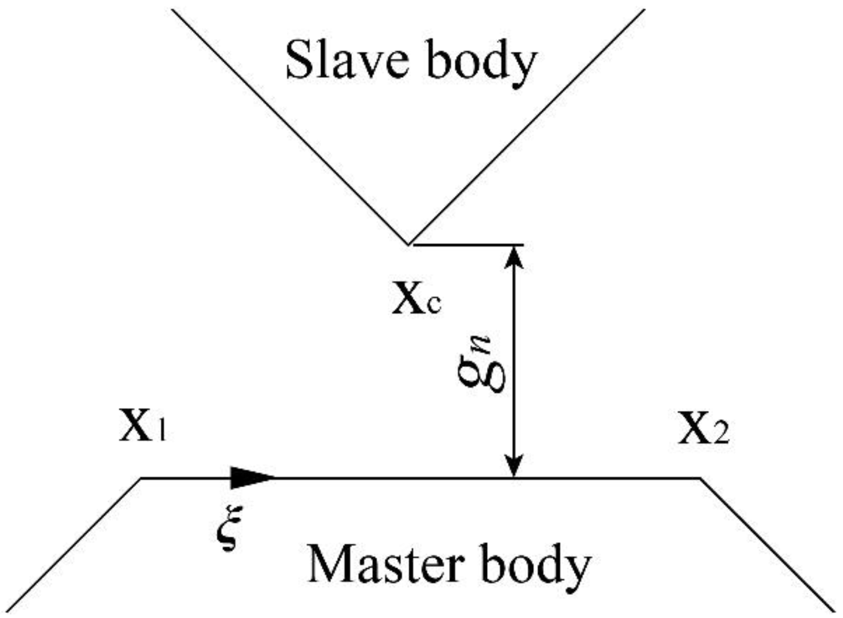
2. Implementation of the Penalty Method in the FEM

In this paper, the commonly used method, i.e., the penalty method, is utilised to solve the contact problems. In the penalty method, a small amount of penetration is allowed, and the contact force is proportional to the amount of penetration. In order to combine the penalty method with the FEM, the slave-master concept is introduced in the FEM.

In the slave-master concept, one of the two contact bodies is designated as a slave body and the other one is a master body, as shown in Figure 1. In FEM, one node from the slave body and two nodes from the master body are defined as one contact pair. In one contact pair, the first objective is to check whether the slave node X_c is in contact with the master segment X₁X₂, i.e., the gap g_n is positive (separated) or negative (in contact). If it is in contact, the contact forces at the slave node and the master nodes will be calculated by the penalty method. In addition, the contact stiffness at the three nodes will also be calculated.

After the contact search is finished, the stiffness and forces calculated by the penalty method will be added into the matrix equation as [26]:

$$\left(\mathit{K}+{\mathit{K}}_{\mathit{c}}\right)∆{\mathit{u}}_{\mathit{g}}={\mathit{F}}_{\mathit{r}\mathit{e}\mathit{s}}+F_c$$

(1)

where, K_c is the contact stiffness matrix in the global coordinate, F_c is the contact force in the global coordinate, while K is the global stiffness matrix in the FEM and F_res is the residual force in the FEM generated from boundary conditions. In each contact pair (one slave node with one master segment), the contact stiffness matrix k_c can be calculated as:

$${\mathit{k}}_{\mathit{c}}={\mathit{k}}_{\mathit{N}}+{\mathit{k}}_{\mathit{T}}$$

(2)

in which, k_N and k_T are the stiffness matrices due to normal contact and consideration of friction, respectively.

$${\mathit{k}}_{\mathit{N}}={\omega }_n{\mathit{C}}_{\mathit{n}}{\mathit{C}}_{\mathit{n}}^T$$

(3)

For the calculation of k_T, there are two different situations: the stick situation and the slip situation. For the stick condition,

$${\mathit{k}}_{\mathit{T}}={\omega }_t{\mathit{C}}_{\mathit{t}}{\mathit{C}}_{\mathit{t}}^T+\frac{{\omega }_t{g}_t}{l}\left({\mathit{C}}_{\mathit{n}}{\mathit{P}}^T+\mathit{P}{\mathit{C}}_{\mathit{n}}^T-{\mathit{C}}_{\mathit{t}}{\mathit{Q}}^{\mathit{T}}-\mathit{Q}{\mathit{C}}_{\mathit{t}}^T\right)$$

(4)

$$g_t=l^0\left(\xi -{\xi }^0\right)$$

(5)

in which, $\xi$ is the local coordinate of the projection point of the slave node on the master surface (see Figure 1). The superscript ‘⁰’ denotes the previous time step. $l^0$ is the length of the master segment.

For the slip condition,

$${\mathit{k}}_{\mathit{T}}=\mu {\omega }_n\mathrm{sgn}\left(g_t\right){\mathit{C}}_{\mathit{t}}{\mathit{C}}_{\mathit{N}}^T+\frac{{\omega }_t{g}_t}{l}\left({\mathit{C}}_{\mathit{n}}{\mathit{P}}^T+\mathit{P}{\mathit{C}}_{\mathit{n}}^T-{\mathit{C}}_{\mathit{t}}{\mathit{Q}}^T-\mathit{Q}{\mathit{C}}_{\mathit{t}}^T\right)$$

(6)

In addition, the contact force of each contact pair for the stick condition can be calculated as:

$${\mathit{f}}_{\mathit{c}}=-{\omega }_n{g}_n{\mathit{C}}_{\mathit{n}}-{\omega }_t{g}_t{\mathit{C}}_{\mathit{t}}$$

(7)

The contact force of each contact pair for the slip condition can be calculated as:

$${\mathit{f}}_{\mathit{c}}=-{\omega }_n{g}_n{\mathit{C}}_{\mathit{n}}-\mu {\omega }_n{g}_n\mathrm{sgn}\left(g_t\right){\mathit{C}}_{\mathit{t}}$$

(8)

In the above equations, the vectors C_n, C_t, P, Q are defined as follows:

$${\mathit{C}}_{\mathit{n}}=\mathit{N}-\frac{g_n}{l}\mathit{Q}$$

$${\mathit{C}}_{\mathit{t}}=\mathit{T}+\frac{g_n}{l}\mathit{P}$$

$$\mathit{N}=\left[\begin{array}{c}{\mathit{e}}_{\mathit{n}}\\ -\left(1-\xi \right){\mathit{e}}_{\mathit{n}}\\ -\xi {\mathit{e}}_{\mathit{n}}\end{array}\right],T=\left[\begin{array}{c}{\mathit{e}}_{\mathit{t}}\\ -\left(1-\xi \right){\mathit{e}}_{\mathit{t}}\\ -\xi {\mathit{e}}_{\mathit{t}}\end{array}\right],P=\left[\begin{array}{c}\mathbf{0}\\ -{\mathit{e}}_{\mathit{n}}\\ {\mathit{e}}_{\mathit{n}}\end{array}\right],N=\left[\begin{array}{c}\mathbf{0}\\ -{\mathit{e}}_{\mathit{t}}\\ {\mathit{e}}_{\mathit{t}}\end{array}\right]$$

(9)

where, ω_n and ω_t are the penalty parameters, e_n is the unit normal vector and e_t is the unit tangential vector. The detailed derivation of K_c and F_c is referred to in Chapter 5 in Kim [26].

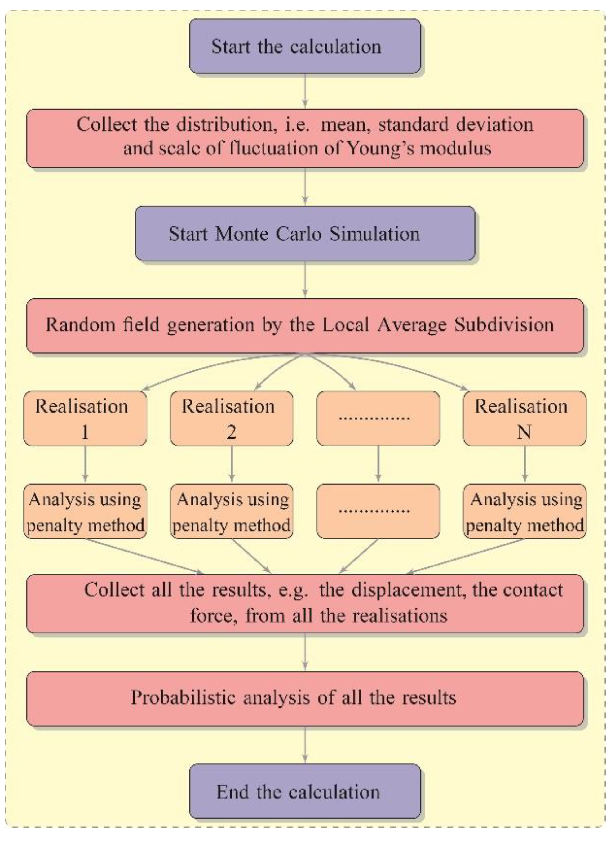
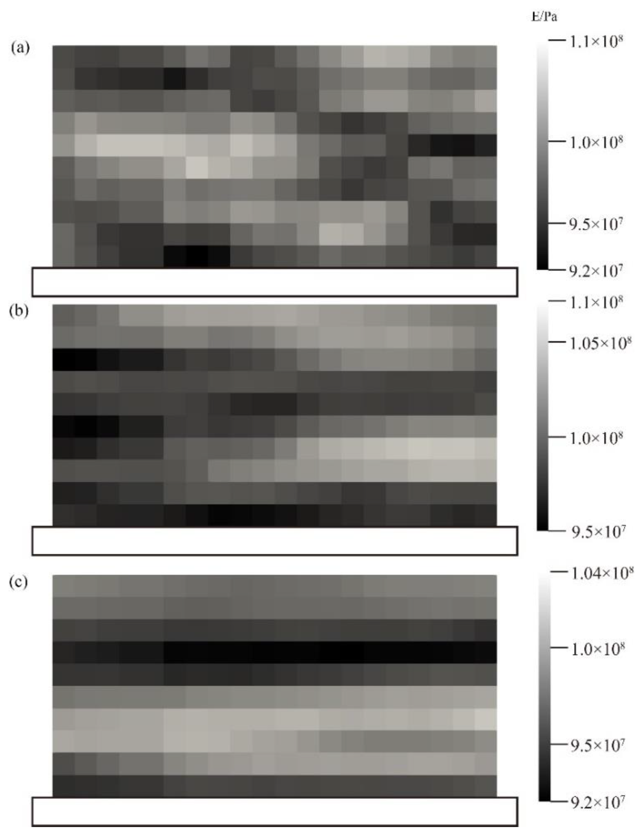
3. Radom Field Generation

In this paper, the LAS method [27] is undertaken to model the heterogeneity of soil parameters. The implementation of the LAS requires the information of soil parameters, which is the distribution of parameters (i.e., the mean and standard deviation). The LAS can generate standard normal random fields first, then these fields can be transformed to the required fields, which follows the input distribution.

In addition to the distribution of the soil parameters, in order to model the correlation of parameter values of two points, the scales of fluctuation in the vertical and horizontal directions are also indispensable. The scales of fluctuation are used to build the correlation function used in the LAS. In this paper, an exponential Markov correlation function is taken as follows:

$$\rho \left({\tau }_1,{\tau }_2\right)=\exp \left(-\sqrt{{\left(\frac{2{\tau }_v}{{\theta }_v}\right)}^2+{\left(\frac{2{\tau }_h}{{\theta }_h}\right)}^2}\right)$$

(10)

where, $\rho \left({\tau }_1,{\tau }_2\right)$ is the correlation coefficient between the values of two points, ${\tau }_v$ and ${\tau }_h$ are the lag distance between two points in the vertical and horizontal directions in a random field, respectively. ${\theta }_v$ and ${\theta }_h$ are the vertical and horizontal scales of fluctuation, respectively. The reader refers to Samy [28] and Spencer [29] for the detailed implementation of the LAS in FEM.

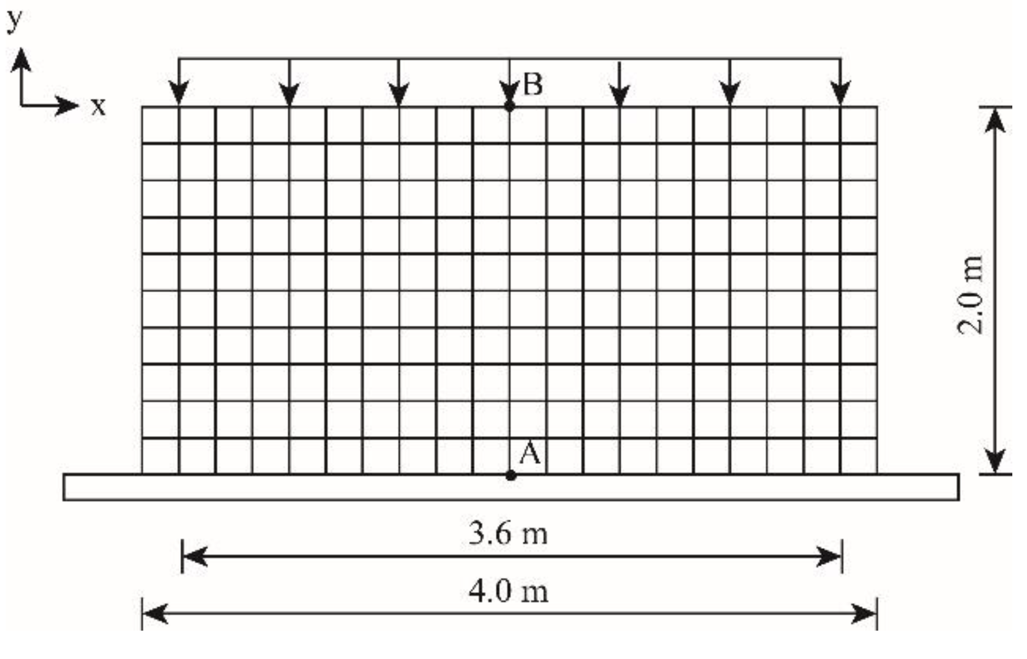
4. Illustrative Example

In this paper, a simple plane-strain contact problem is analysed as an example. Figure 2 shows the flowchart of using the proposed method to analyse the illustrative example. The LAS is first used to generate multiple realisations of the random field, and then each realisation is imported to the contact analysis using the penalty method. Finally, all the results from all the realisations are collected and analysed. In this example, an elastic block is pressed against a rigid foundation, which is extracted from the contact between the overlying soil and the concrete lining in tunnels. The elastic block is 4 m long and 2 m high. On the top of the elastic block, there is a uniformly distributed load. The uniformly distributed load is 200 kN/m. The finite element mesh for this problem is shown in Figure 3, and the size of the mesh is 0.2 m by 0.2 m. Each element has 4 nodes. In this example, the Poisson’s ratio ν is 0.3. Young’s modulus is taken to be a random variable, which follows a normal distribution.

4.1. Validation of the Numerical Results

In order to validate the program used in this paper, the results computed by the program are compared with the results obtained from the widely used commercial software Abaqus. In this comparison, two scenarios have been selected: in the first scenario, there is no friction along the interface, and in the second one the coefficient of friction of the interface is 0.3. In both cases, Young’s modulus is assumed to be uniform across the whole research domain and equal to the mean of Young’s modulus.

Figure 4 shows the comparison between the results of the program and the results of Abaqus. The light blue line with the blank circle and the grey line with the blank triangle show the results of the normal contact force for the first scenario. The light red line with blank square and the orange line with cross show the normal contact force for the second scenario. The blue line with the solid circle and the green line with solid diamond show the frictional contact force for the second scenario. From Figure 4, the results computed by the program are close to the results of Abaqus, which proves the validity of the program.

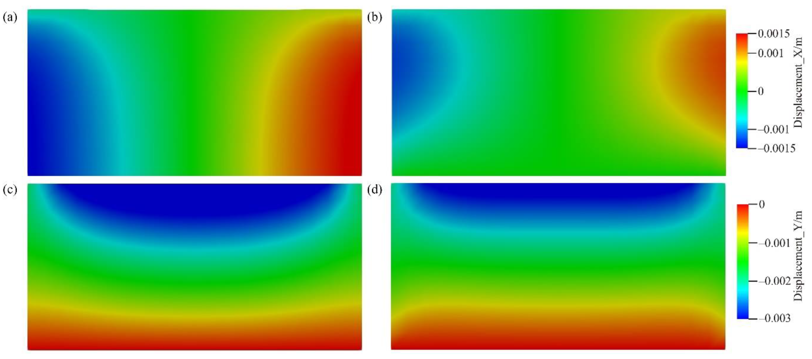
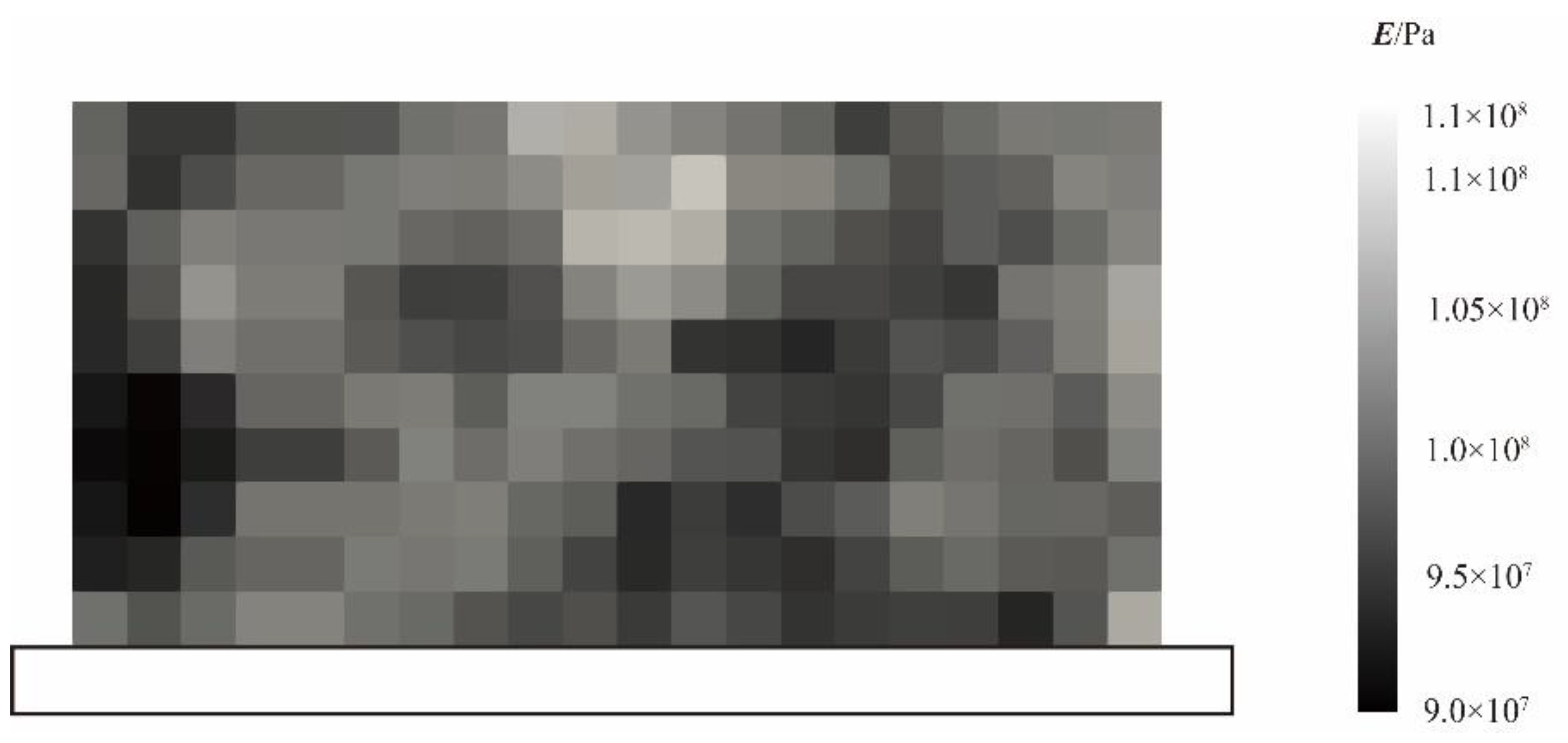
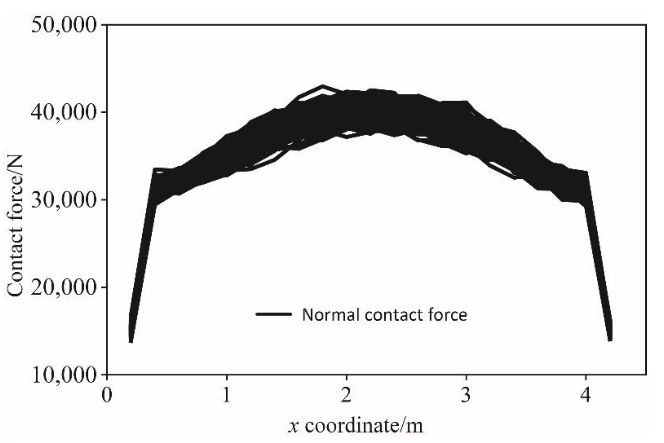
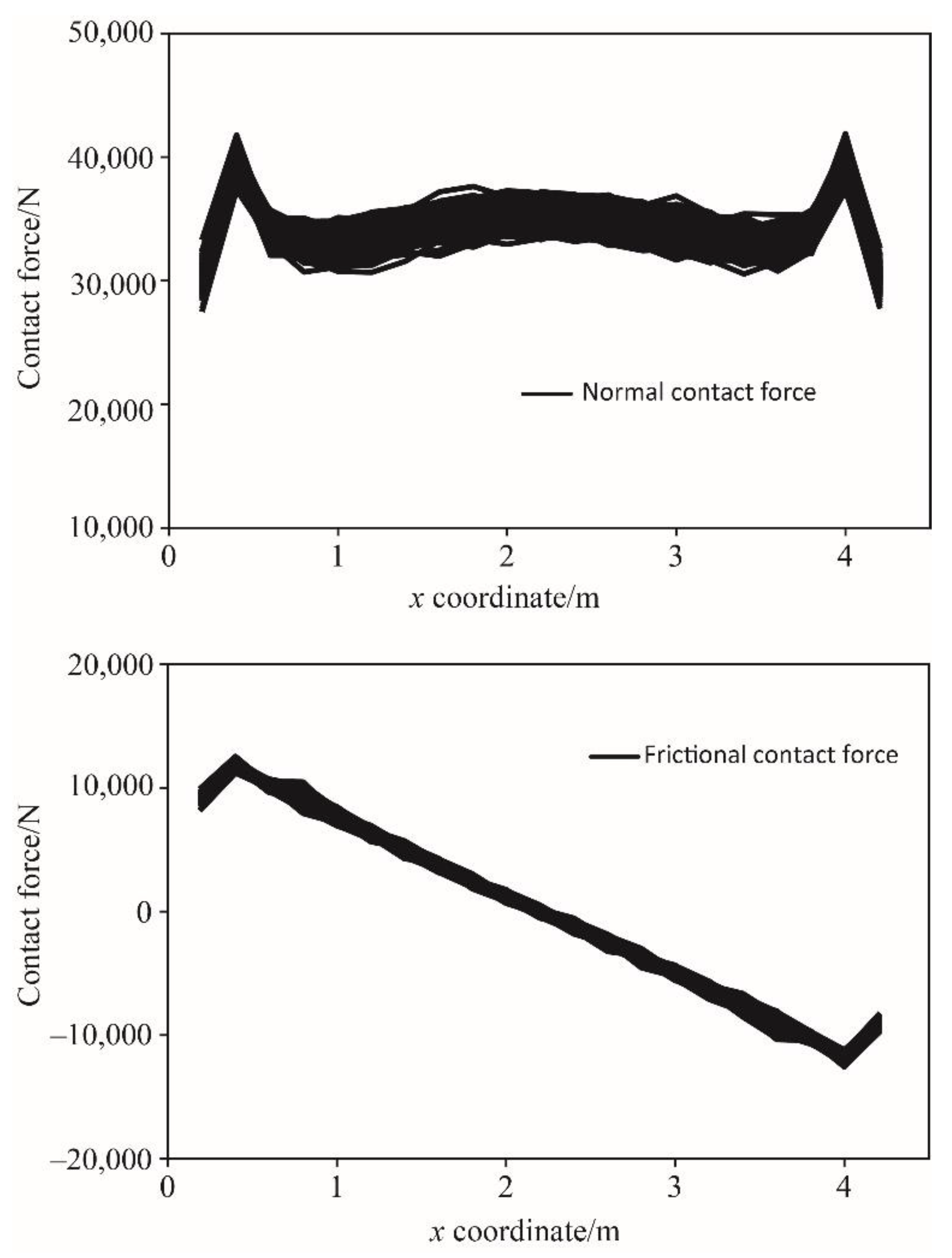
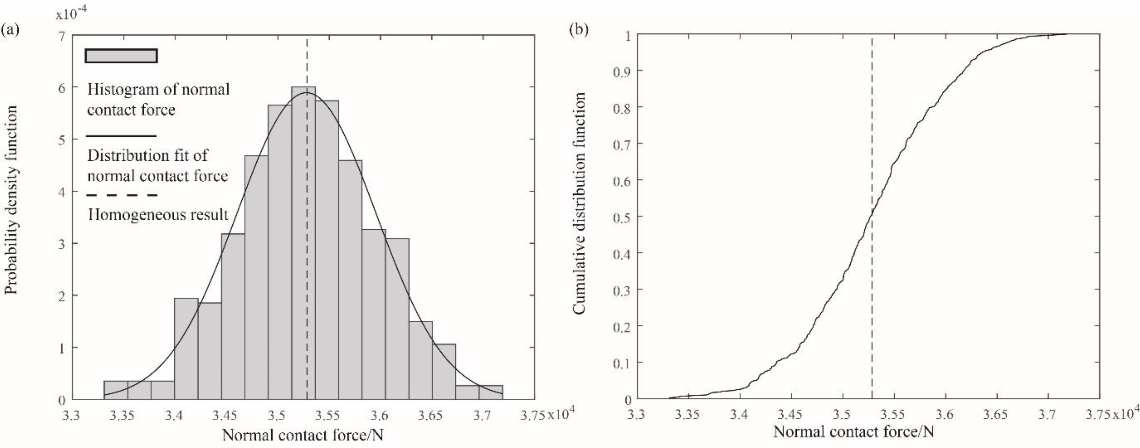
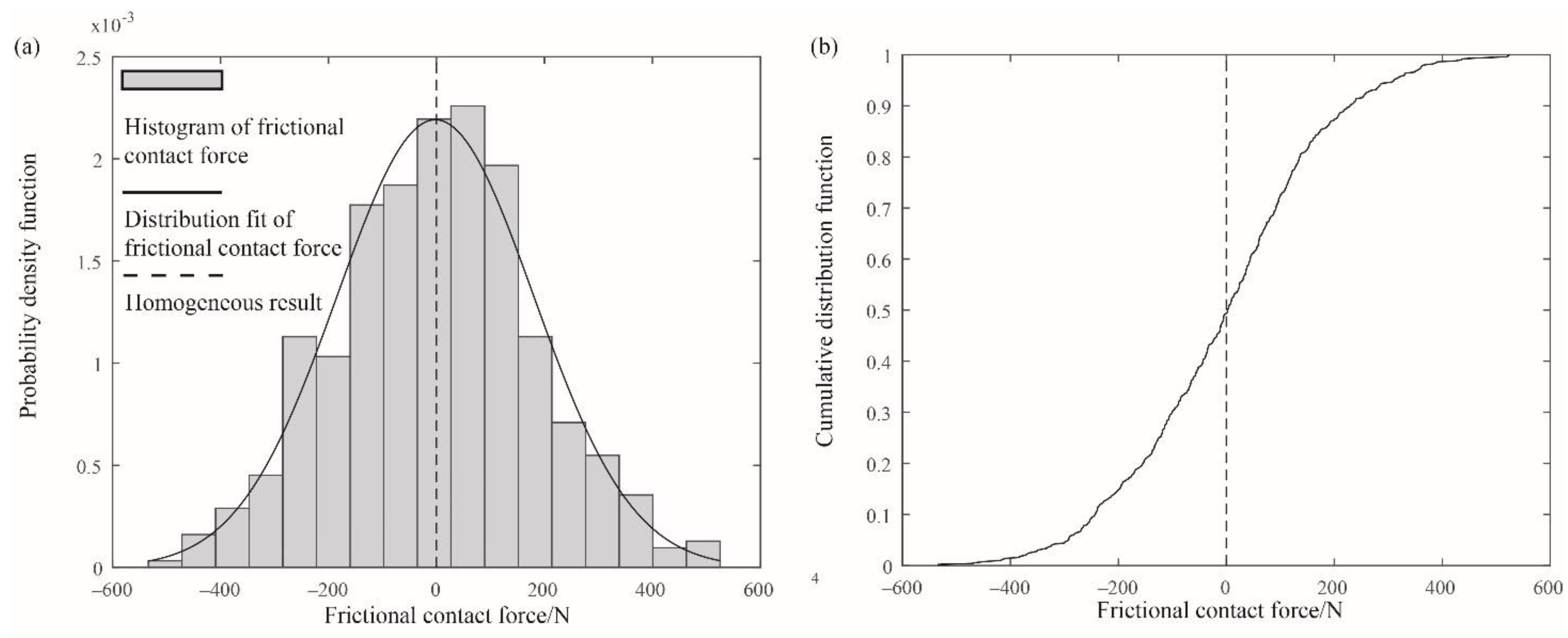
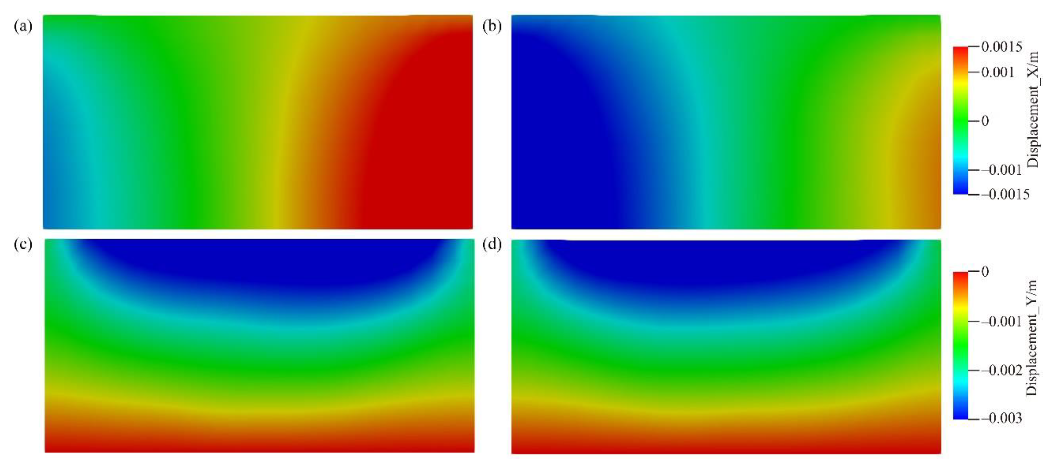
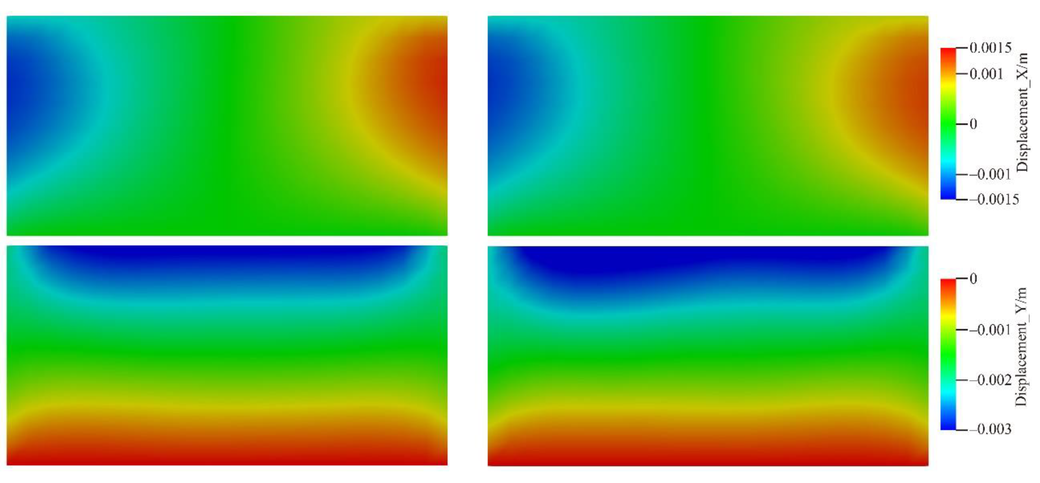
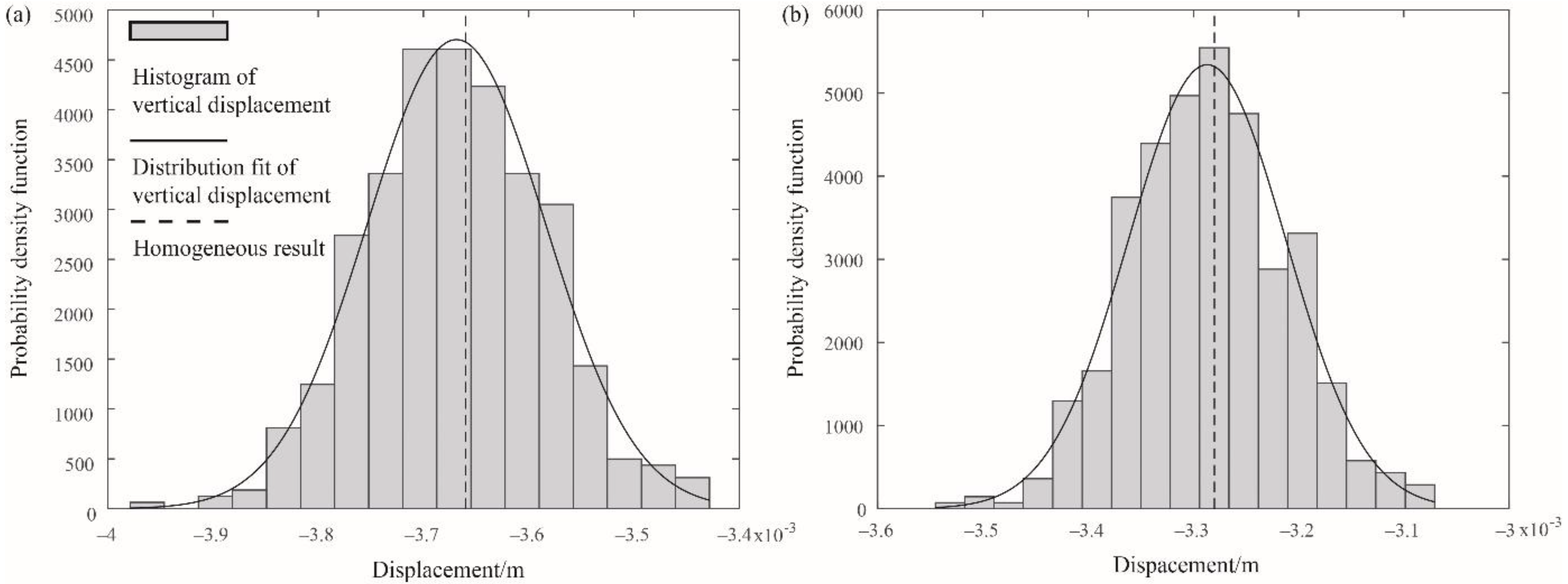
4.2. Comparison between the Homogeneous Case and Heterogeneous Case

In order to investigate the influence of heterogeneity on the contact problems, a homogeneous case is analysed first. As in the previous subsection, Figure 4 presents the results of the homogeneous case, which are the computed contact force applied on the bottom of the elastic block along the interface when the coefficient of friction is 0.0 and 0.3. From Figure 4, it can be seen the normal contact force is symmetrical when the Young’s modulus is uniform. In addition, Figure 5 shows the deformation of the elastic block under loading for both scenarios.

Figure 5a,b show the horizontal displacement when the coefficients of friction are 0.0 and 0.3, respectively. Figure 5c,d show the vertical displacement. It can be seen from Figure 5 that the horizontal/vertical displacement is symmetrical. However, due to the emergence of friction, the distribution of the displacement across the whole domain is quite different. From Figure 5a,b, it can be found that because of the friction, the shape of the zone with large horizontal displacement becomes significantly smaller. The horizontal displacement reduces much near the interface. Moreover, Figure 5c,d indicate that the shape of the zone with large vertical displacement changes as well. In addition, the maximum horizontal and vertical displacements of the case with no friction are larger than those of the case when the coefficient of friction is 0.3.

Then, Young’s modulus of the elastic block is assumed to be spatially variable. The mean and coefficient of variation (COV) (defined as the standard deviation divided by the mean) of Young’s modulus are 100 MPa and 5%, respectively. Additionally, the scale of fluctuation of Young’s modulus is chosen to be 1.0 m. Figure 6 shows one realisation of the random field. From Figure 6, each finite element mesh has been assigned with a different value. In this paper, the total number of realisations used in the computation is 500. In each realisation, the contact forces can be calculated.

Figure 7 and Figure 8 show the results of contact forces from 500 realisations when there is no friction and the coefficient of friction is 0.3, respectively. From Figure 7 and Figure 8, it can be found that the heterogeneity of Young’s modulus has a significant influence on the results of contact force. First, due to the spatial variability of Young’s modulus, the distribution of normal contact force along the contact surface is not symmetrical. Moreover, Figure 6 and Figure 7 show that the COV of the contact force at a specific point changes with the x coordinate. Furthermore, it can be seen from Figure 8 that the variation of the frictional contact force is less than that of the normal contact force, which suggests that the influence of heterogeneity has more of an impact on the normal contact force.

Later, to investigate the detailed variation of the contact forces at each point, the normal contact force at the middle bottom point A (shown in Figure 3) of the elastic block has been selected as an example. The following Figure 9, Figure 10 and Figure 11 show the normal and frictional contact force at the point A of the elastic block from 500 realisations when the coefficient of friction is 0 and 0.3, respectively. In the homogeneous case, the normal contact forces at the point A for two scenarios (one has no friction, and the coefficient of friction is 0.3 in the other one) are 40,099.7 N and 35,283.8 N. From Figure 9a, Figure 10a and Figure 11a, it can be found that the distribution of the contact forces follows a normal distribution. When there is no friction, the mean and the standard deviation of the normal contact force are 40,068 N and 835.6 N. When the coefficient of friction is 0.3, the mean and the standard deviation of the normal contact force are 35,279 N and 677.2 N. Meanwhile, the mean and the standard deviation of the frictional contact force are −2.0746 N and 182.1 N. The contact force of the homogeneous case is quite close to the mean of the heterogeneous case. By comparing Figure 9a and 10a, it can be seen that the contact with no friction generally has larger normal contact forces, which is consistent with the homogeneous case. In addition, from Figure 9b and Figure 10b, the probability of the contact force exceeding a certain value can be calculated. For example, in the scenario without friction, if the normal contact force of the homogeneous case (40,099.7 N) is taken as a limit, the probability of exceeding the limit is 1 − P (normal contact force < 40,099.7 N), i.e., 48.2% in this paper. Similarly, when the coefficient of friction is 0.3, if the normal contact force of the homogeneous case (35,283.8 N) is taken as a limit, the probability of exceeding the limit is 49.8%. When the coefficient of friction is 0.3, if the frictional contact force of the homogeneous case (0 N) is taken as a limit, the probability of exceeding the limit is 51%.

Since the influence of heterogeneity on the contact force is significant, the heterogeneity certainly has an influence on the corresponding displacement of the elastic block. Figure 12 shows the displacement of the elastic block from two realisations when there is no friction. Comparing Figure 12 with Figure 5a,c, it can be seen that the displacement of the heterogeneous case is significantly different from that of the homogeneous case. For the horizontal and vertical displacements, the variation of the horizontal displacement is much more obvious. Figure 13 shows the displacement of the elastic block from two realisations when the coefficient of friction is 0.3. From the figure, the variation of the horizontal and vertical displacements is not significant compared to the scenario with no friction.

The variation of the vertical displacement is not obvious; in order to better investigate the influence, the vertical displacement of the middle top point B (shown in Figure 3) has been selected as an example. The vertical displacements of the homogeneous cases are −0.00366 m (no friction) and −0.00328 m (the coefficient of friction is 0.3), respectively. The following Figure 14 has shown the PDF of the vertical displacement at the point B when the coefficients of friction are 0 and 0.3, respectively. From Figure 14, it can be seen that the variation of the vertical displacement follows a normal distribution. When there is no friction, the mean and the standard deviation of the vertical displacement are −0.00367 m and −0.0000848 m. The mean is quite close to the result of the homogeneous case (−0.00366 m). When the coefficient of friction is 0.3, the mean and the standard deviation of the vertical displacement is −0.00329 m and −0.0000747 m. The mean is also close to the result of the homogeneous case (−0.00328 m).

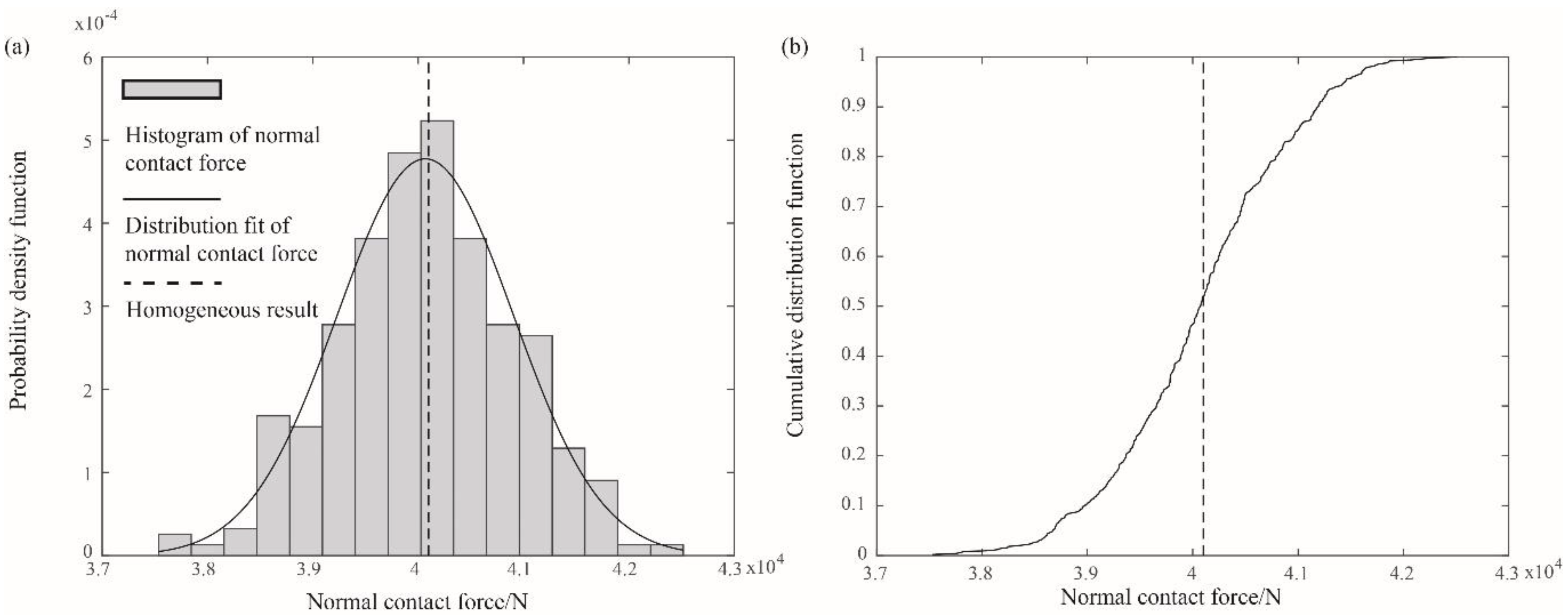
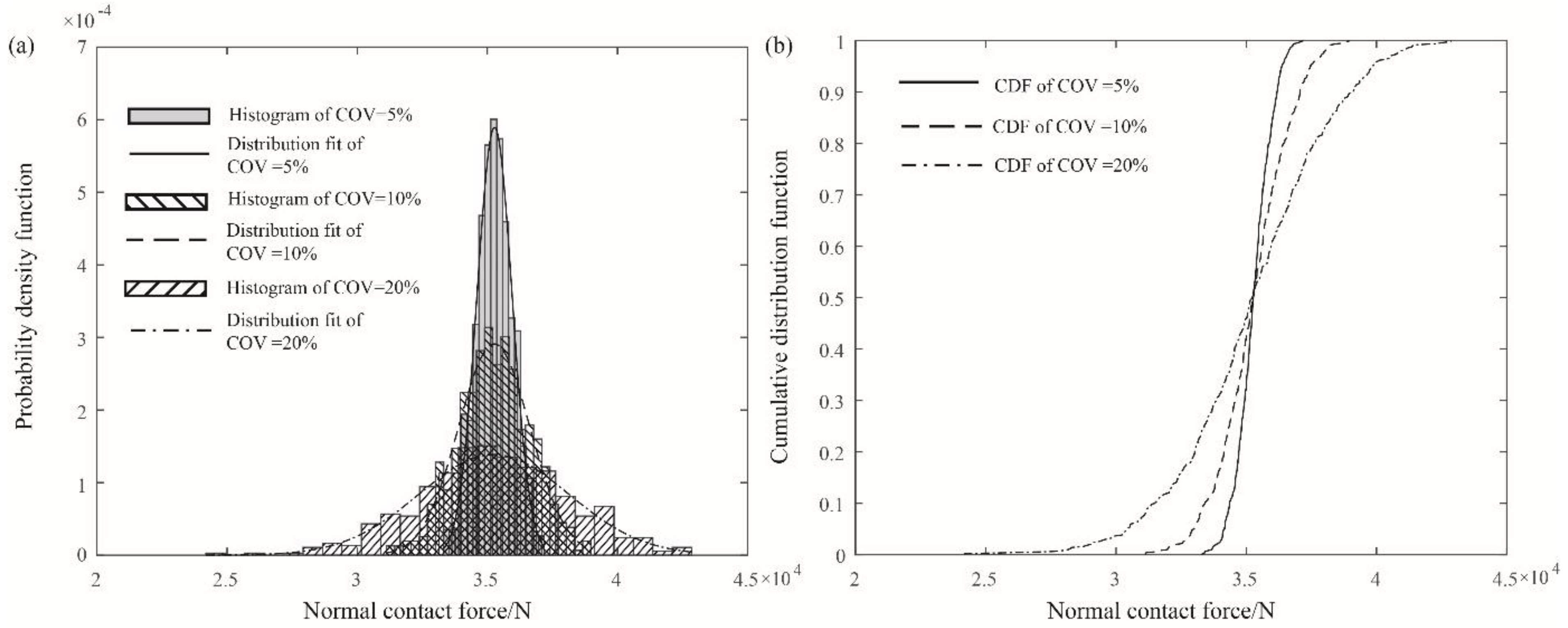
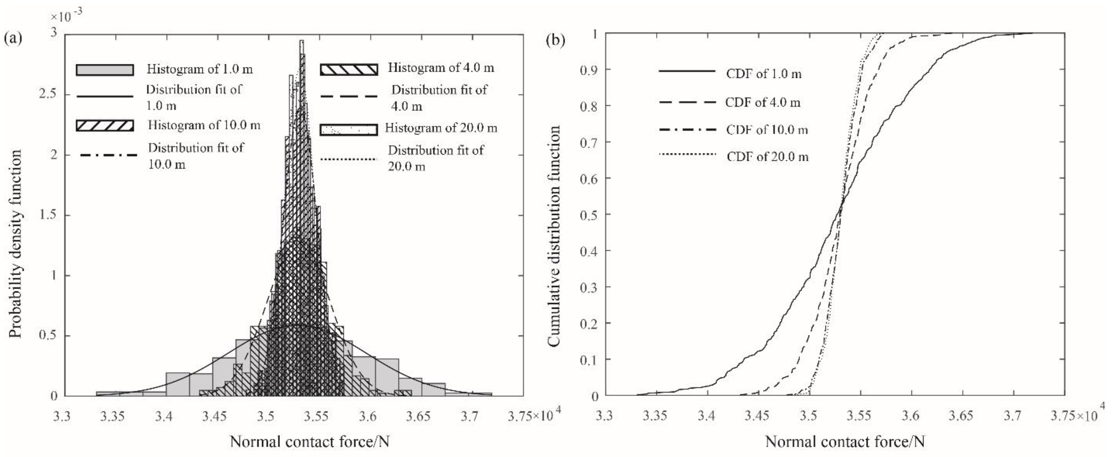
4.3. Influence of the Statistics of Young’s Modulus on the Contact Force

The previous subsection has demonstrated the influence of the heterogeneity on the results of contact force and displacement. The random field generation is controlled by the statistics of Young’s modulus, i.e., the mean, the COV and the scale of fluctuation. Therefore, in this subsection, the purpose is to investigate the influence of different standard deviation and different scale of fluctuation.

First, the influence of different standard deviation is investigated. The COV of Young’s modulus is chosen to be 5% (which has been used in the previous subsection), 10% and 20%, respectively. In the investigation, the coefficient of friction remains 0.3 and the scale of fluctuation is assumed to be 1.0 m. Figure 15 shows the PDFs and CDFs of the normal contact force at the point A when the COV is 5%, 10% and 20%. From Figure 15, it proves that with the increase of the COV of Young’s modulus, the mean of the normal contact force does not have significant variation, whereas the standard deviation of the normal contact force increases. It is because that with the increase of the COV, the range of the value of Young’s modulus becomes wider. When the COV is 5%, the mean and the standard deviation of the normal contact force are 35,279 N and 677.2 N. When the COV is 10%, the mean and the standard deviation of the normal contact force are 35,266 N and 1371.3 N. When the COV is 20%, the mean and the standard deviation of the normal contact force are 35,255 N and 2878.4 N.

Second, the influence of the scale of fluctuation is investigated. The horizontal scale of fluctuation is chosen to be 1.0 m (which has been used in the previous subsection), 4.0 m 10.0 m and 20 m, respectively. The vertical scale of fluctuation remains 1.0 m. In the comparison, the coefficient of friction remains as 0.3 and the COV is assumed to be 5%. Figure 16 shows the random field with different horizontal scales of fluctuation, i.e., 4.0 m, 10.0 m and 20.0 m. It can be seen that the distribution of Young’s modulus across the whole domain is different from each other. With the increase of the horizontal scale of fluctuation, the Young’s modulus of any two distant points becomes more correlated.

In Figure 17, it shows the PDFs and CDFs of the normal contact force at the point A when the horizontal scales of fluctuation are 1.0 m, 4.0 m, 10.0 m and 20.0 m. It can be found from the figure that the standard deviation of the normal contact force decreases with the increase of the horizontal scale of fluctuation, whereas the increase of the horizontal scale of fluctuation has no significant influence on the mean.

Table 1. Mean and standard deviation of the normal contact force for different horizontal scales of fluctuation.

Horizontal Scale of Fluctuation (m)	Mean of the Normal Contact Force (N)	Standard Deviation of the Normal Contact Force (N)
1.0	35,279	677.2
4.0	35,292	310.8
10.0	35,308	166.8
20.0	35,304	147.0

has shown the mean and standard deviation of the normal contact force for different horizontal scale of fluctuation. The reason could be that with the increase of the horizontal scale of fluctuation, the value of Young’s modulus along the horizontal direction varies less, which can be seen in Figure 16c, so less variation causes decreases in the standard deviation.

5. Conclusions

In this paper, a simple elastic problem has been studied to investigate the influence of heterogeneity on the contact forces and deformation. It is the first time that the linking the penalty method has been used with the LAS. In the example, the parameter Young’s modulus has been considered as a spatial variable. The penalty method and the LAS have been linked together to solve the contact problem and model the heterogeneity of Young’s modulus.

First, in the homogeneous case in which Young’s modulus is taken to be uniform across the whole research domain, it can be found that the normal/frictional contact force and the deformation is symmetrical. Compared to the homogeneous case, the results of the case where Young’s modulus is considered to be spatially variable (following a normal distribution) shows that the influence of soil heterogeneity on the elastic contact problems is significant. Due to heterogeneity, the contact force and deformation shows evident variation. The variation of the normal contact force at any specific point follows a normal distribution, and the COV changes with the x coordinate. When the soils are considered to be heterogenous, it can be found that there is a certain probability when the contact force exceeds a certain value (result calculated in the homogeneous case). This implies that the conventional analysis of the contact problems in which the soils are taken as homogeneous could induce risk. In addition, the variation of the frictional contact force is less than that of the normal contact force.

Later, the influences of different COVs and horizontal scales of fluctuation have been investigated. The results show that with the increase of the COV of Young’s modulus, the standard deviation of the normal contact force increases. However, with the increase of the horizontal scale of fluctuation of Young’s modulus, the standard deviation of the normal contact force decreases.

From the analysed results, it suggests that, in order to better predict the deformation/stress in the contact bodies (such as soil–concrete contact), the spatial variability needs to be considered. To achieve this, the proposed approach of linking the penalty method with the LAS can be applied.

References

1. Zhang, B.Y.; Wang, J.G.; Shi, R. Time-dependent deformation in high concrete-faced rock-fill dam and separation between concrete face slab and cushion layer. Comput. Geotech. 2004, 31, 559–573. [Google Scholar] [CrossRef]
2. Liu, S.H.; Wang, L.J.; Wang, Z.J.; Bauer, E. Numerical stress-deformation analysis of cut-off wall in clay-core rockfill dam on thick overburden. Water Sci. Eng. 2016, 9, 219–226. [Google Scholar] [CrossRef]
3. Youakim, S.A.S.; El-Metewally, S.E.E.; Chen, W.F. Nonlinear analysis of tunnels in clayey/sandy soil with a concrete lining. Eng. Struct. 2000, 22, 707–722. [Google Scholar] [CrossRef]
4. Goodman, R.E.; Taylor, R.L.; Brekke, T.L. A model for the mechanics of jointed rock. J. Soil Mech. Found. Div. 1968, 94, 637–659. [Google Scholar] [CrossRef]
5. Desai, C.S.; Zaman, M.M.; Lightner, J.G.; Siriwardane, H.J. Thin-layer element for interfaces and joints. Int. J. Numer. Anal. Methods Geomech. 1984, 8, 19–43. [Google Scholar] [CrossRef]
6. Hughes, T.J.R.; Taylor, R.L.; Sackman, J.L.; Curnier, A.; Kanoknukulchai, W. A finite element method for a class of contact-impact problems. Comput. Methods Appl. Mech. Eng. 1976, 8, 249–276. [Google Scholar] [CrossRef]
7. Papadopoulos, P.; Solberg, J.M. A Lagrange multiplier method for the finite element solution of frictionless contact problems. Math. Comput. Model. 1998, 28, 373–384. [Google Scholar] [CrossRef]
8. Oysu, C.; Fenner, R.T. Coupled FEM-BEM for elastoplastic contact problems using Lagrange multipliers. Appl. Math. Model. 2006, 30, 231–247. [Google Scholar] [CrossRef]
9. Hansbo, P.; Rashid, A.; Salomonsson, K. Least-squares stabilized augmented Lagrangian multiplier method for elastic contact. Finite Elem. Anal. Des. 2016, 116, 32–37. [Google Scholar] [CrossRef] [Green Version]
10. White, D.J.; Enderby, L.R. Finite-element stress analysis of a non-linear problem: A connecting-road eye loaded by means of a pin. J. Strain Anal. 1970, 5, 41–48. [Google Scholar] [CrossRef]
11. Babuska, I. The finite element method with penalty. Math. Comput. 1973, 27, 221–228. [Google Scholar] [CrossRef] [Green Version]
12. Hird, C.C.; Kwok, C.M. Finite element studies of interface behaviour in reinforced embankments of soft ground. Comput. Geotech. 1989, 8, 111–131. [Google Scholar] [CrossRef]
13. Sharma, K.G.; Desai, C.S. Analysis and implementation of thin-layer element for interfaces and joints. J. Eng. Mech. 1992, 118, 2442–2462. [Google Scholar] [CrossRef]
14. Qian, X.X.; Yuan, H.N.; Li, Q.M.; Zhang, B.Y. Comparative study on interface elements, thin-layer elements, and contact analysis methods in the analysis of high concrete-faced rockfill dams. J. Appl. Math. 2013, 2013, 320890. [Google Scholar] [CrossRef] [Green Version]
15. Weyler, R.; Oliver, J.; Sain, T.; Cante, J.C. On the contact domain method: A comparison of penalty and lagrange multiplier implementations. Comput. Methods Appl. Mech. Eng. 2012, 205–208, 68–82. [Google Scholar] [CrossRef]
16. Zeng, M.H.; Wu, Z.M.; Wang, Y.J. A stochastic model considering heterogeneity and crack propagation in concrete. Constr. Build. Mater. 2020, 254, 119289. [Google Scholar] [CrossRef]
17. Amato, F.; Moscato, V.; Picariello, A.; Sperlí, G. Diffusion algorithms in multimedia social networks: A preliminary model. In Proceedings of the 2017 IEEE/ACM International Conference on Advances in Social Networks Analysis and Mining, Sydney, Australia, 31 July–3 August 2017; pp. 844–851. [Google Scholar]
18. Fenton, G.A.; Griffiths, D.V. Bearing capacity prediction of spatially random cϕ soil. Can. Geotech. J. 2003, 40, 54–65. [Google Scholar] [CrossRef]
19. Cho, S.E.; Park, H.C. Effect of spatial variability of cross-correlated soil properties on bearing capacity of strip footing. Int. J. Numer. Anal. Methods Geomech. 2010, 34, 1–26. [Google Scholar] [CrossRef]
20. Griffiths, D.V.; Fenton, G.A. Seepage beneath water retaining structures founded on spatially random soil. Géotechnique 1993, 43, 577–587. [Google Scholar] [CrossRef] [Green Version]
21. Liu, K.; Vardon, P.J.; Hicks, M.A. Sequential reduction of slope stability uncertainty based on temporal hydraulic measurements via the ensemble Kalman filter. Comput. Geotech. 2017, 95, 147–161. [Google Scholar] [CrossRef] [Green Version]
22. Yetbarek, E.; Kumar, S.; Ojha, R. Effects of soil heterogeneity on subsurface water movement in agricultural fields: A numerical study. J. Hydrol. 2020, 590, 125420. [Google Scholar] [CrossRef]
23. Hicks, M.A.; Li, Y. Influence of length effect on embankment slope reliability in 3D. Int. J. Numer. Anal. Methods Geomech. 2018, 42, 891–915. [Google Scholar]
24. ElGhoraiby, M.A.; Manzari, M.T. The effects of base motion variability and soil heterogeneity on lateral spreading of mildly sloping ground. Soil Dyn. Earthq. Eng. 2020, 135, 106185. [Google Scholar] [CrossRef]
25. Fenton, G.A. Error evaluation of three random-field generators. J. Eng. Mech. 1994, 120, 2478–2497. [Google Scholar] [CrossRef]
26. Kim, N.H. Introduction to Nonlinear Finite Element Analysis; Springer: New York, NY, USA, 2015. [Google Scholar]
27. Fenton, G.A.; Vanmarcke, E.H. Simulation of random fields via local average subdivision. J. Eng. Mech. 1990, 116, 1733–1749. [Google Scholar] [CrossRef] [Green Version]
28. Samy, K. Stochastic Analysis with Finite Elements in Geotechnical Engineering; University of Manchester: Manchester, UK, 2003. [Google Scholar]
29. Spencer, W.A. Parallel Stochastic and Finite Element Modelling of Clay Slope Stability in 3D; University of Manchester: Manchester, UK, 2007. [Google Scholar]
Figure 1. Contact of two bodies.
Applsci 11 04240 g001
Figure 2. Flowchart of the proposed method.
Applsci 11 04240 g002
Figure 3. Geometry of contact between an elastic block and a rigid foundation, and finite element meshes.
Applsci 11 04240 g003
Figure 4. Validation of the contact results computed by the program.
Applsci 11 04240 g004
Figure 5. Horizontal (a,b) and vertical (c,d) displacements of the elastic block when the coefficient of friction is 0.0 and 0.3.
Applsci 11 04240 g005
Figure 6. One realisation of the random field of Young’s modulus.
Applsci 11 04240 g006
Figure 7. Contact force from 500 realisations when the coefficient of friction is 0.
Applsci 11 04240 g007
Figure 8. Contact force from 500 realisations when the coefficient of friction is 0.3.
Applsci 11 04240 g008
Figure 9. Probability density function (PDF) (a) and cumulative distribution function (CDF) (b) of the normal contact force at the middle bottom point A of the elastic block from 500 realisations when the coefficient of friction is 0.
Applsci 11 04240 g009
Figure 10. PDF (a) and CDF (b) of the normal contact force at the middle bottom point A of the elastic block from 500 realisations when the coefficient of friction is 0.3.
Applsci 11 04240 g010
Figure 11. PDF (a) and CDF (b) of the frictional contact force at the middle bottom point A of the elastic block from 500 realisations when the coefficient of friction is 0.3.
Applsci 11 04240 g011
Figure 12. Horizontal (a,b) and vertical (c,d) displacements of two realisations when the coefficient of friction is 0.
Applsci 11 04240 g012
Figure 13. Horizontal (a,b) and vertical (c,d) displacements of two realisations when the coefficient of friction is 0.3.
Applsci 11 04240 g013
Figure 14. PDFs of the vertical displacement at the middle top point B of the elastic block from 500 realisations when the coefficient of friction is 0 (a) and 0.3 (b).
Applsci 11 04240 g014
Figure 15. PDFs (a) and CDFs (b) of the normal contact force at the point A of the elastic block when the COVs are 5%, 10% and 20%.
Applsci 11 04240 g015
Figure 16. Realisations of the random field for different horizontal scales of fluctuation (a) 4.0 m, (b) 10.0 m and (c) 20.0 m.
Applsci 11 04240 g016
Figure 17. PDFs (a) and CDFs (b) of the normal contact force at the point A of the elastic block when the horizontal scales of fluctuation are 1.0 m, 4.0 m, 10.0 m and 20.0 m.
Applsci 11 04240 g017