
Short-Term Solar Power Forecasting Using Genetic Algorithms: An Application Using South African Data


Abstract
1. Introduction
Background
2. An Overview of the Literature on Solar Forecasting
Research Highlights
- Based on the RMSE and rRMSE, GA was found to be the best model. However, based on MAE and rMAE, RNN was the best model.
- From the Diebold–Mariano tests, the null hypothesis that the forecast accuracy between a pair of forecasts from the two methods is the same was rejected for all the three pairs.
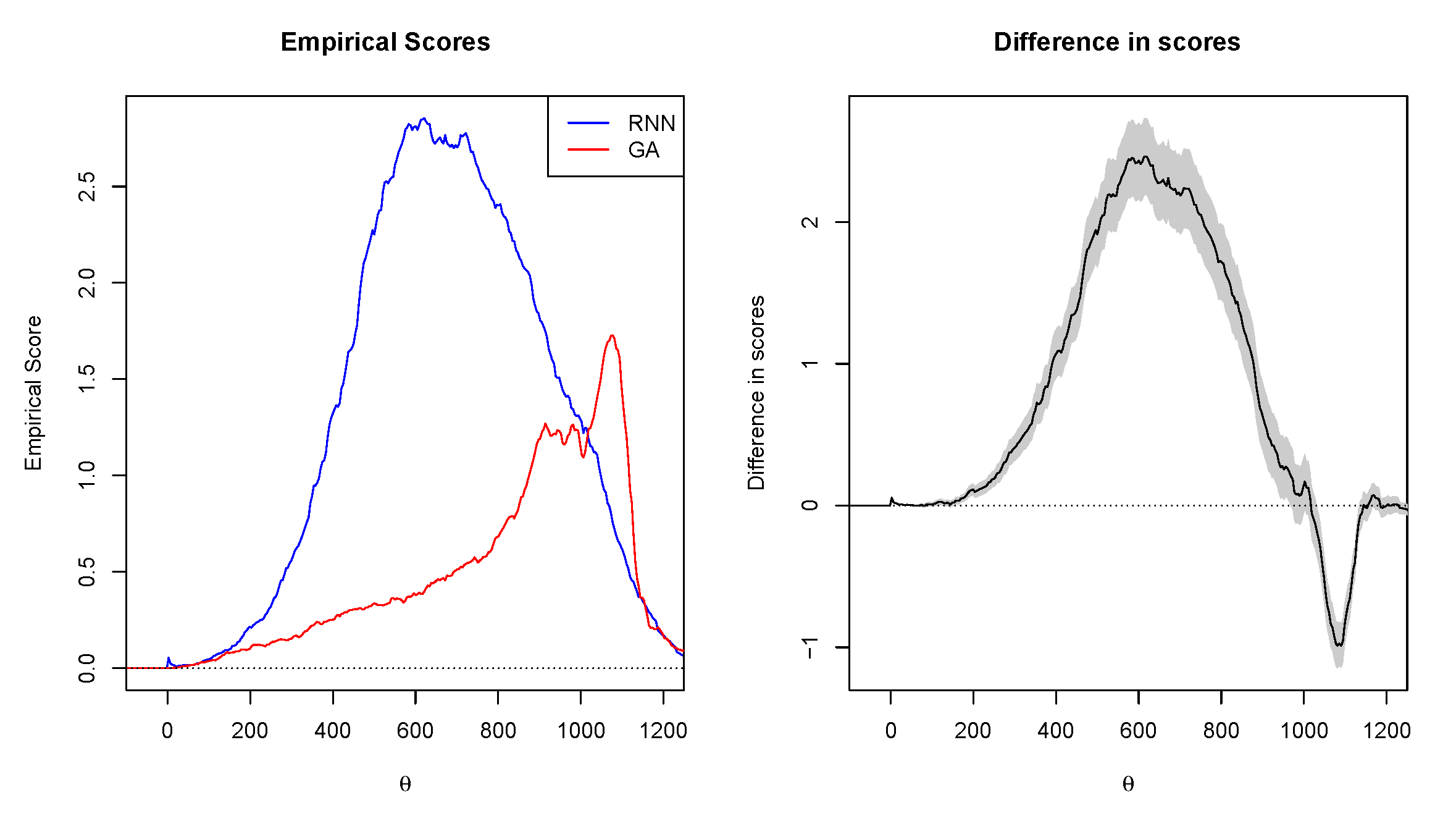
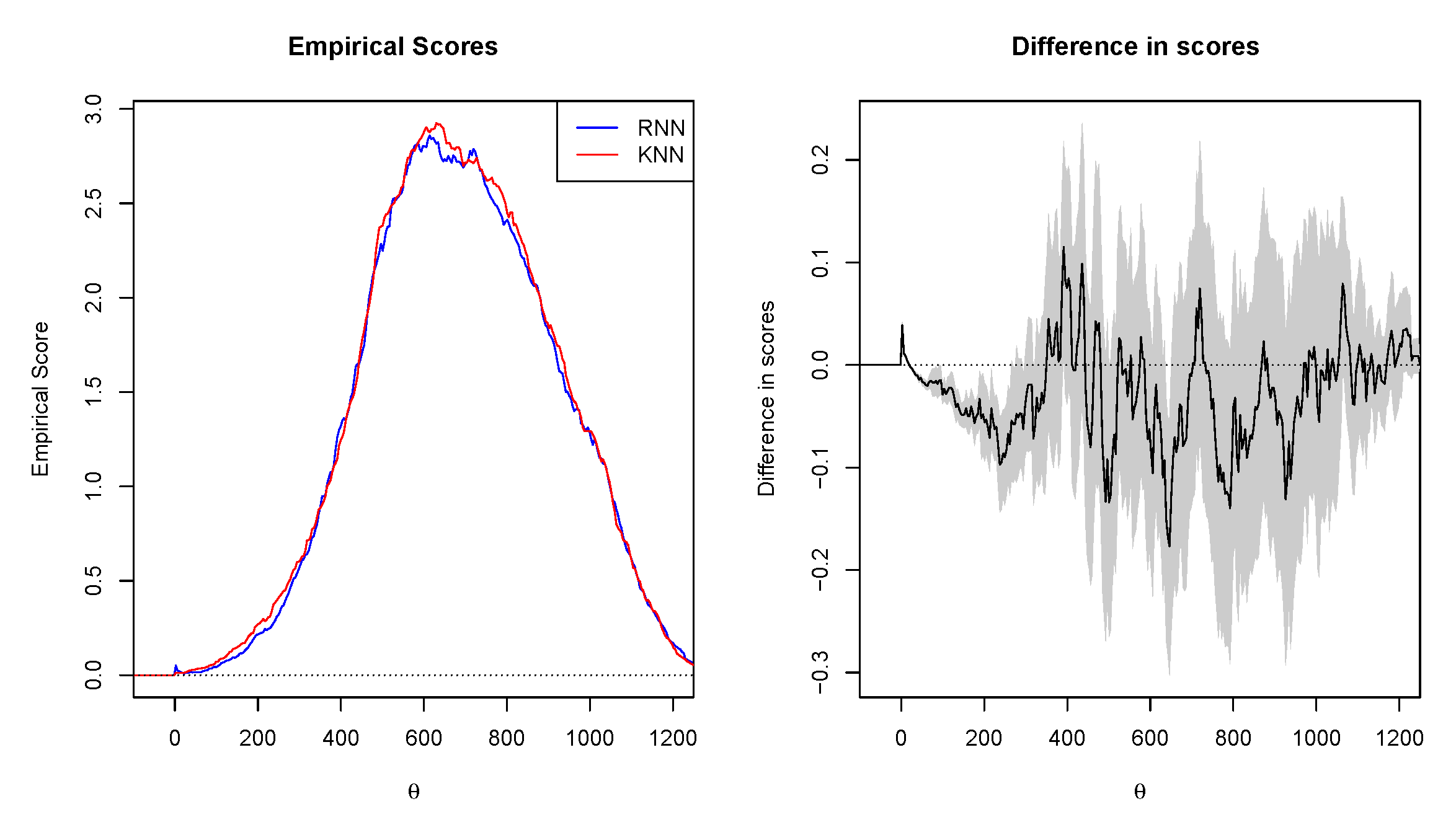
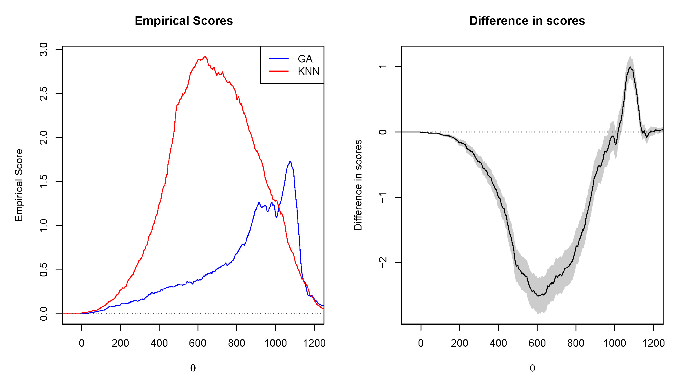
- Based on the Murphy diagrams, the GA dominated both RNN and KNN, meaning that it provides the greatest predictive ability.
- Based on the Giacomini–White tests, GA was found to have the best conditional predictive ability compared to the other two models.
- The results from this paper yield improved results from the previous papers.
- To the best of our knowledge, this is the first paper to compare the genetic algorithm, the K-nearest neighbour method, and recurrent neural networks in short-term forecasting of global horizontal irradiance data from South Africa.
3. Models
3.1. Genetic Algorithm
Implementation of the Genetic Algorithm
- Initially, the time sequence with the sequence of equations for candidate population is given at random.
- Normally, such equations are of the form , with the parameter variables A, B, C, and D are the earlier state variables (, with being the discrete time unit), or the actual values constant, so that the ⨂ symbol is one of the known four basic arithmetic operators .
- Other mathematical operators may be achievable, but increasing the number of accessible operators makes the functional optimisation method difficult.
- A parameter that measures the results of equation strings in a training set is its fitness to the information described by:where is the variance and where is implied by:
- Values of close to one show highly accurate forecasts, whereas low positive or negative values indicate the algorithm’s weak forecast capability.
- The equation strings with a higher number of would be taken to exchange the character string parts among them (reproduction and crossover) in discarding the few unsuitable individuals.
- The offspring is more difficult to produce than the parents.
- The total number of characters throughout the equation strings is upper bounded to avoid the generation of offspring with unreasonable frequency.
- A small proportion of the strong fundamental components, individual operators and variables, of the strings of the equation are progressively mutated at random.
- The process is performed several times to enhance the fitness of the developing population, and the empirical method to estimate function is obtained at the edge of the evolutionary process.
3.2. Recurrent Neural Networks
3.3. Benchmark Models
3.3.1. Implementation of the K-Nearest Neighbours
3.3.2. The KNN Algorithm
- load the solar data from USAid Venda,
- initialise K to the specified number of neighbours,
- for every example in the data,
- calculate the distance between a query example and the current example,
- add the distance and an example index to an ordered set,
- order the set of distances and indices by distances (in ascending order) from the smallest to the largest,
- choose the first K entries in the list which has been sorted,
- get the labels for K entries which have been chosen,
- returns the K label mean if a regression occurs,
- returns the K label mode if it is classified.
3.4. Variable Selection, Parameter Estimation
3.4.1. Variable Selection
3.4.2. The Prediction Intervals
3.4.3. Evaluation of the Prediction Intervals
3.5. Evaluation Metrics
3.6. The Tests for Predictive Accuracy
Diebold–Mariano and Giacomini–White Tests
3.7. Murphy Diagram
3.8. Data and Features
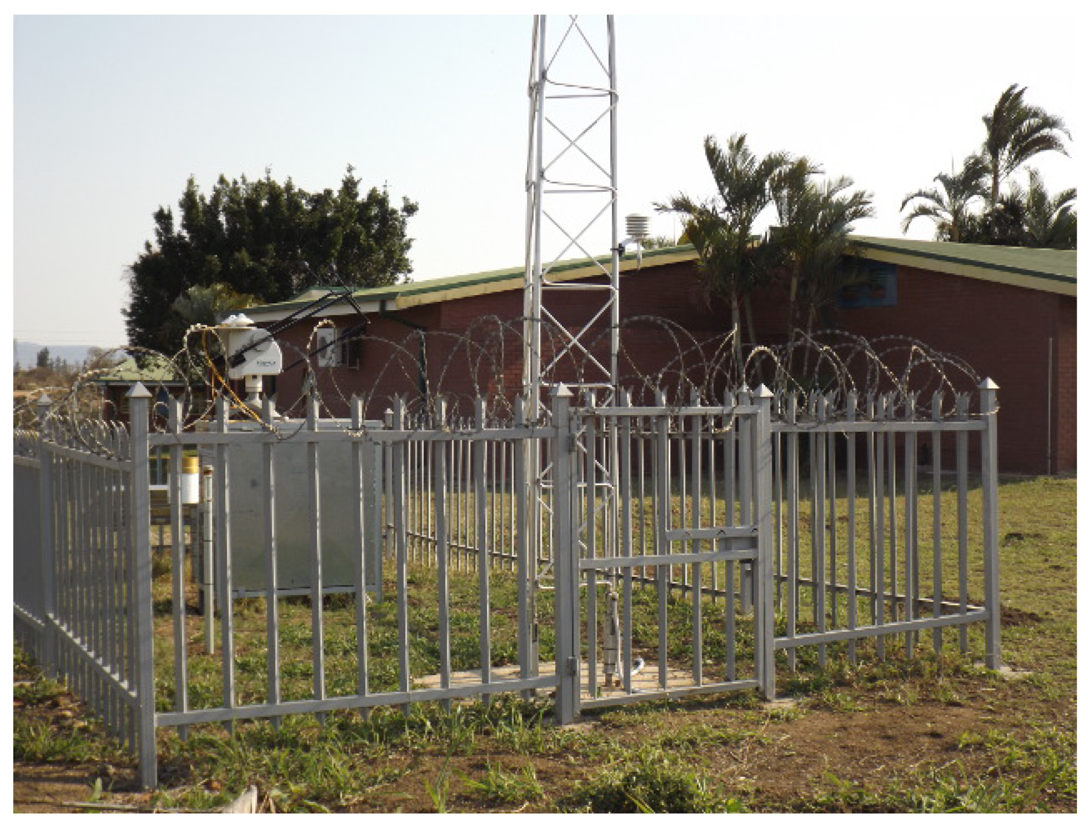
3.8.1. Data
3.8.2. Features
4. Results
4.1. Empirical Results and Discussion
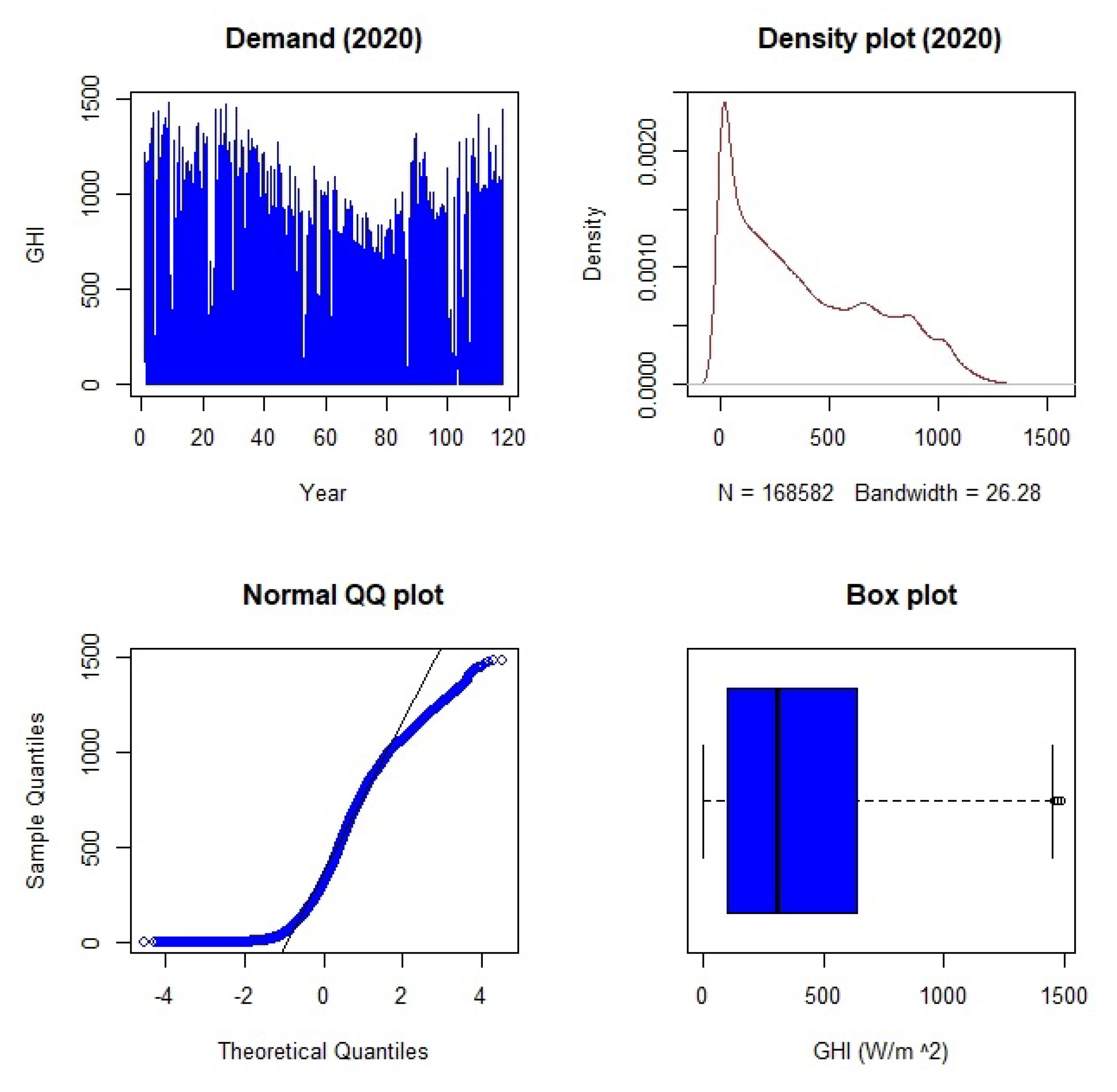
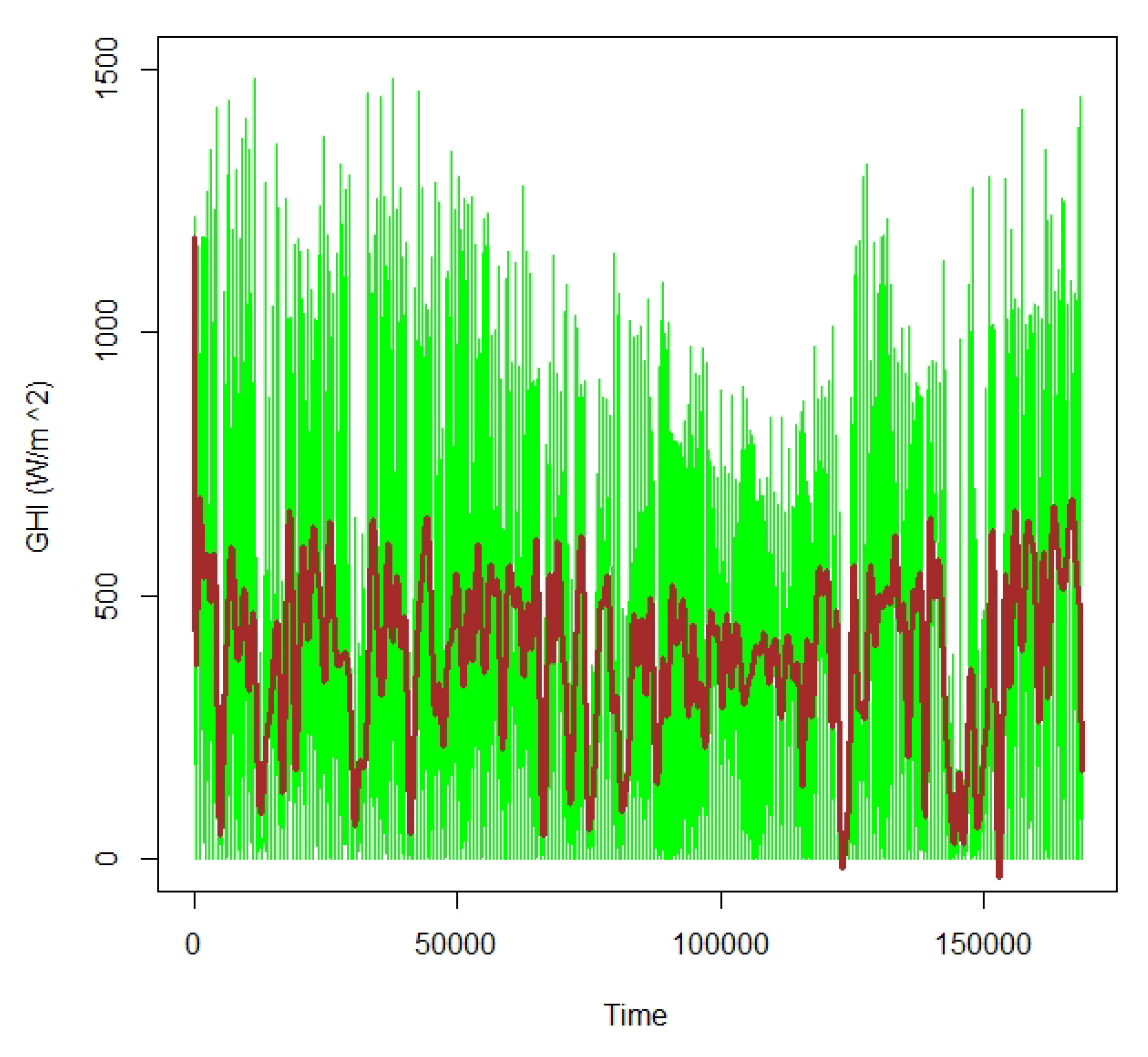
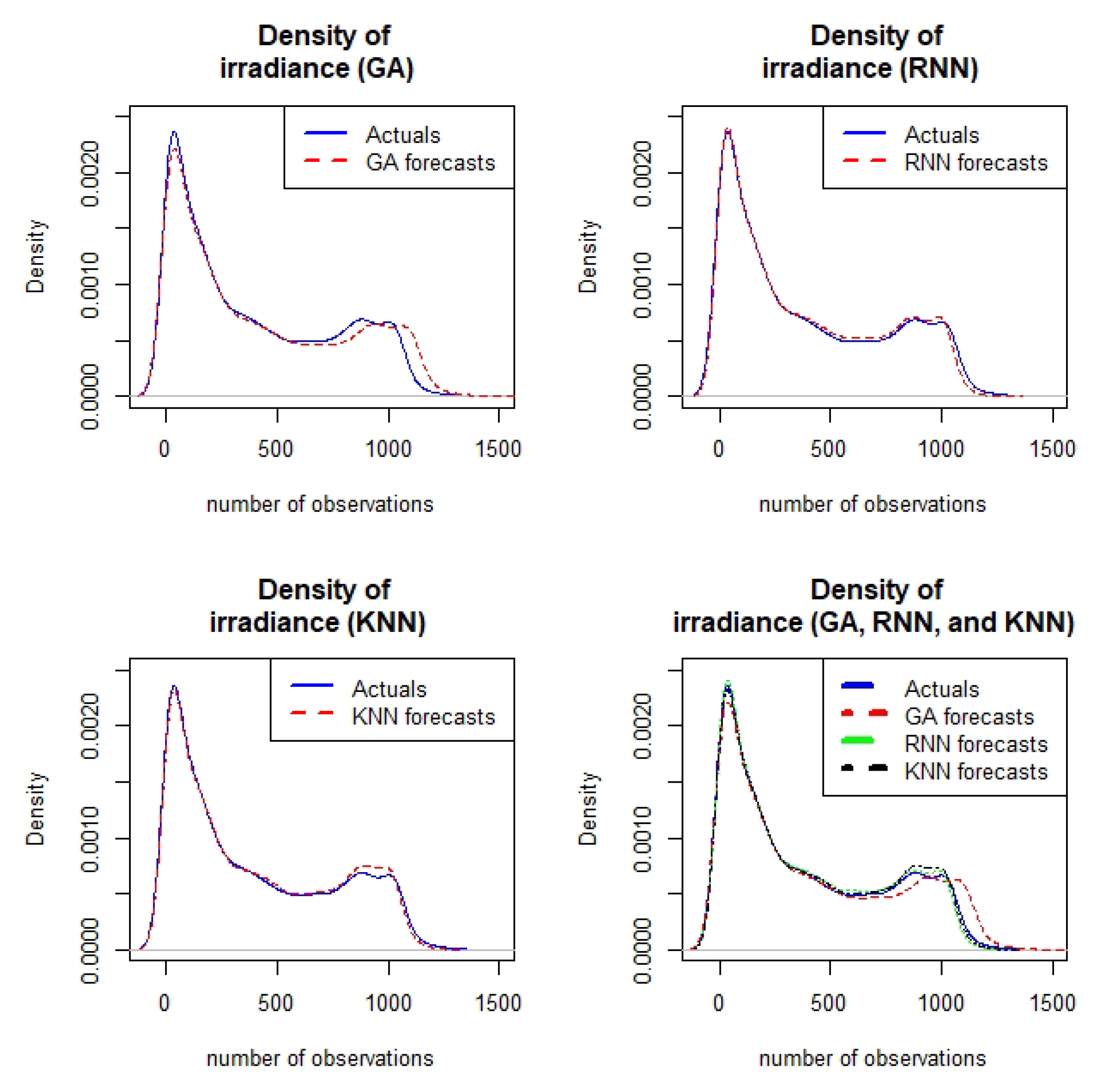
Exploratory Data Analysis
4.2. Variable Selection
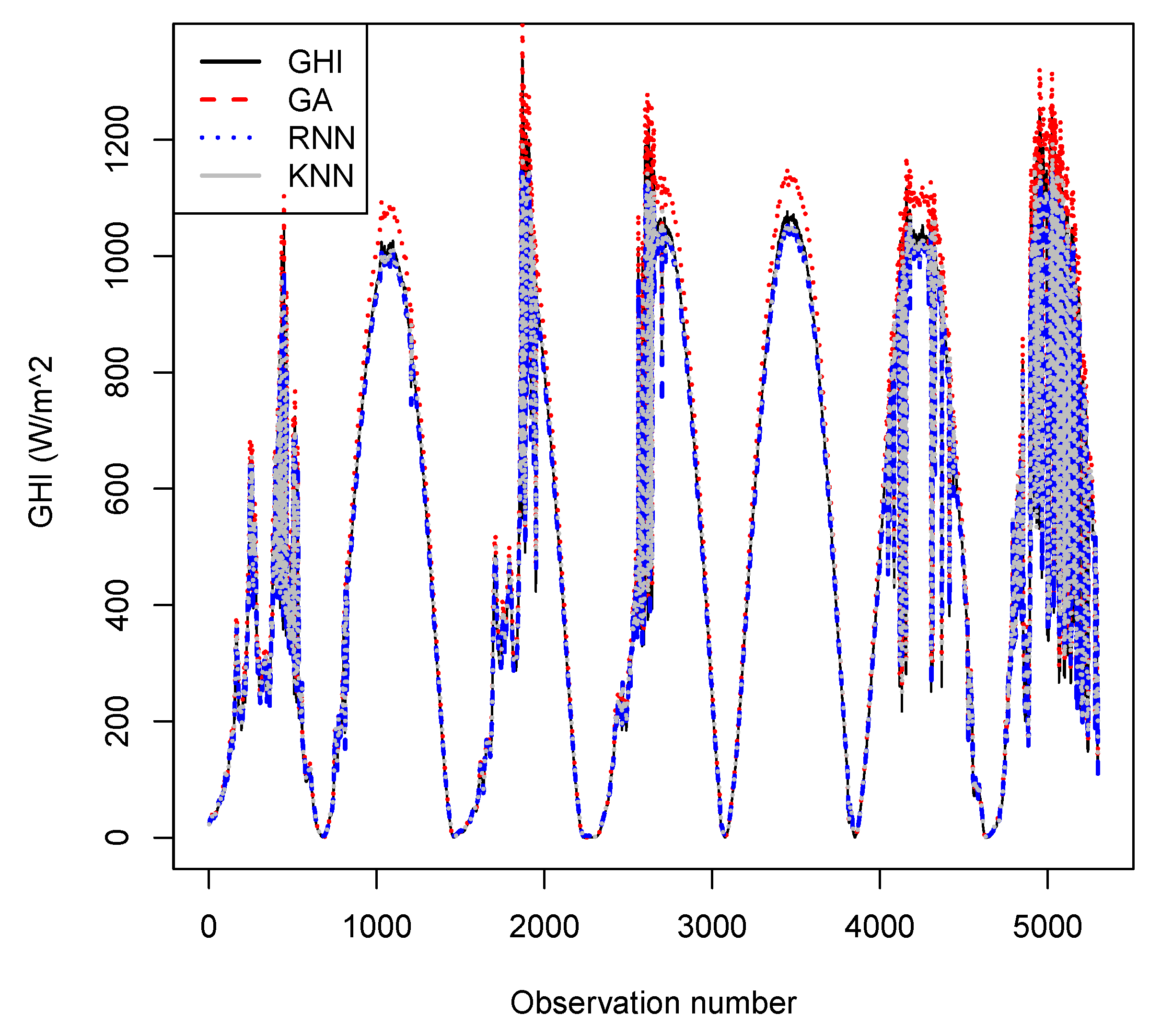
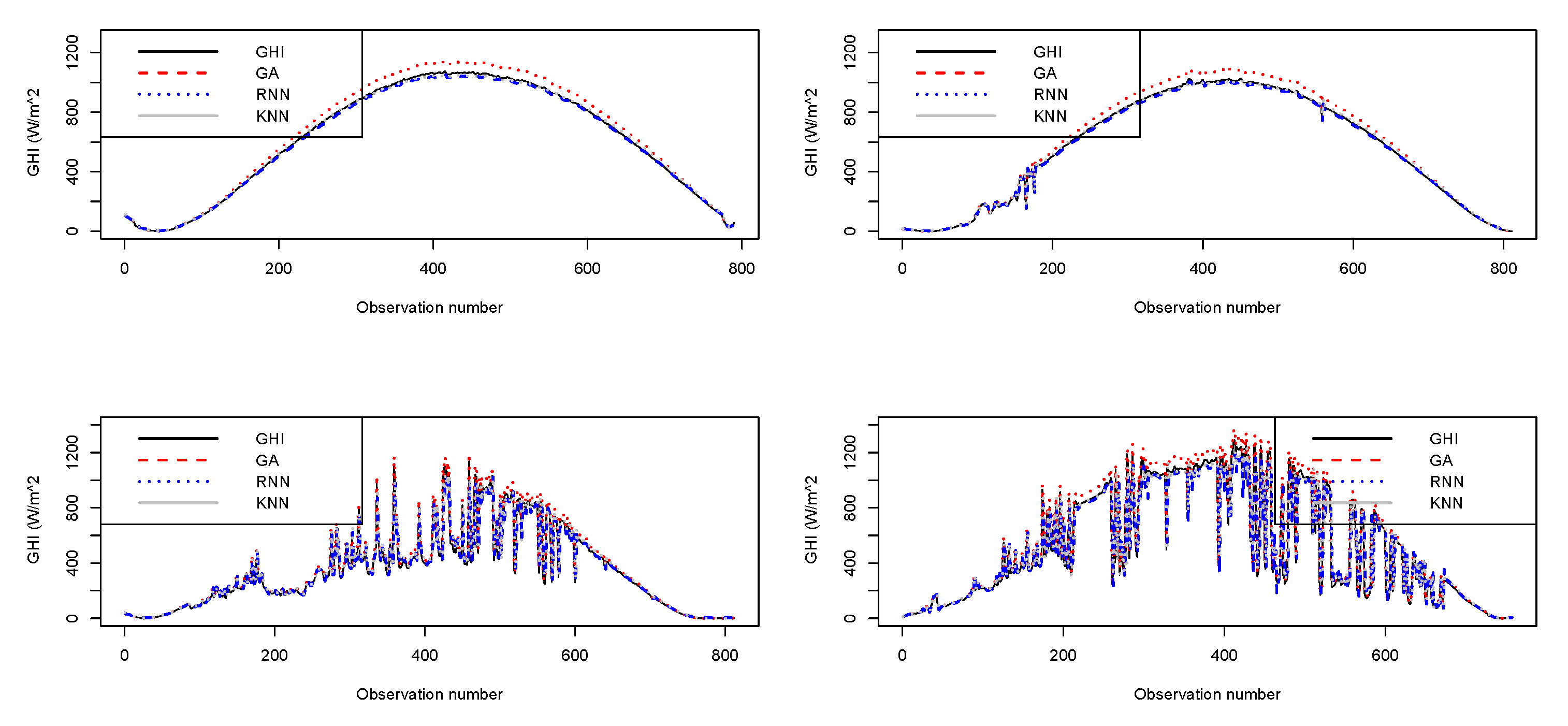
4.3. Forecasting Results
4.4. Models’ Comparative Analysis
4.4.1. Evaluation of Predictive Interval
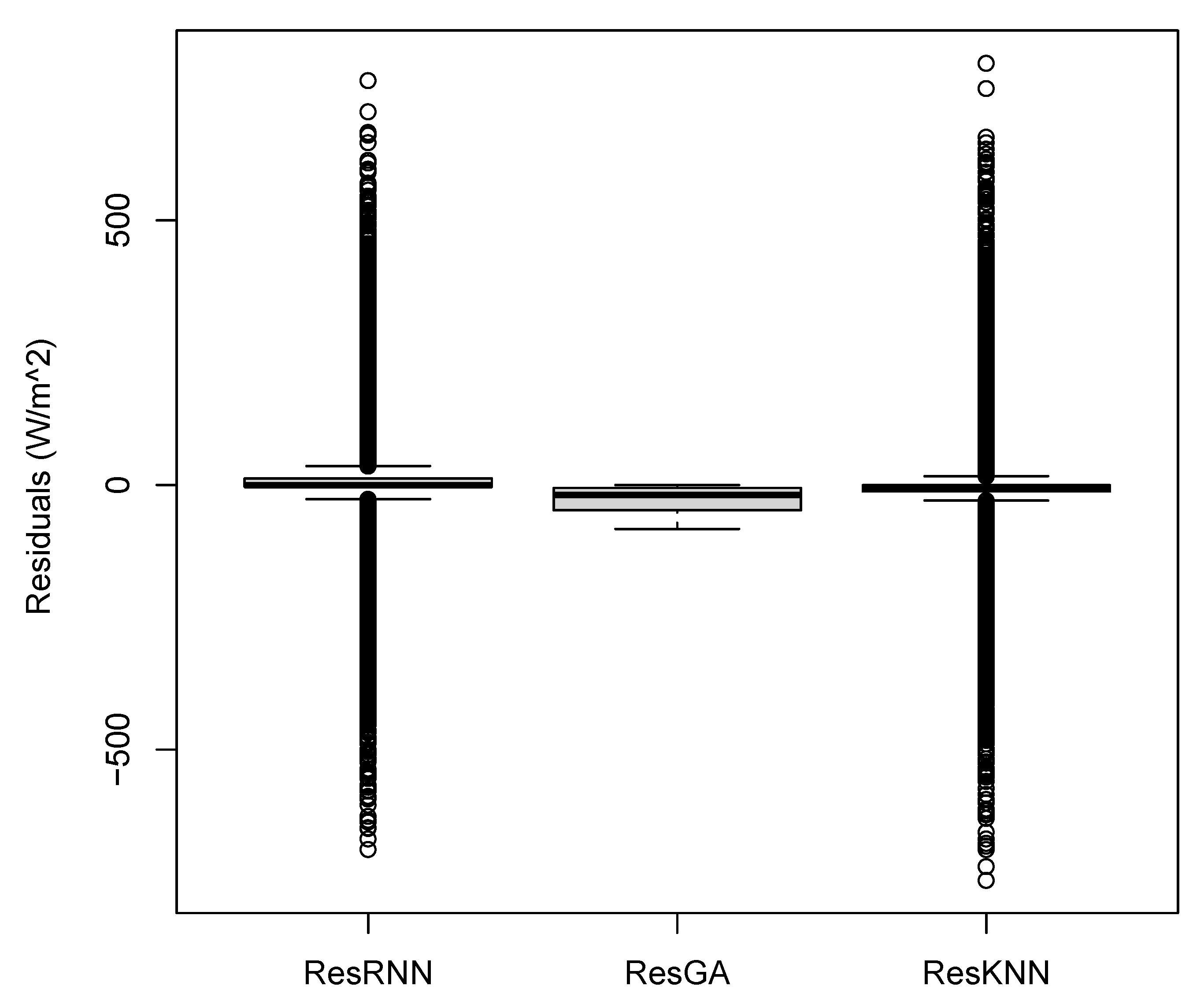
4.4.2. Residual Analysis
4.4.3. Diebold–Mariano Test
4.4.4. Murphy Diagrams
4.4.5. Giacommini–White Test
4.4.6. Discussion of Results
5. Conclusions
Author Contributions
Funding
Institutional Review Board Statement
Informed Consent Statement
Data Availability Statement
Acknowledgments
Conflicts of Interest
Abbreviations
| GA | Genetic Algorithm |
| RNN | Recurrent Neural Network |
| KNN | K-Nearest Neighbour |
| MAE | Mean Absolute Error |
| RMSE | Root Mean Square Error |
| MSE | Mean Square Error |
| rMAE | relative Mean Square Error |
| rRMSE | relative Root Mean Square Error |
| QRA | Quantile Regression Averaging |
| DM | Diebold–Mariano |
| RES | Renewable Energy Source |
| PV | Photovoltaic |
| NWP | Numerical Weather Prediction |
| ANN | Artificial Neural Network |
| SVM | Support Vector Machine |
| CARDS | Combined Autoregressive Furthermore, Dynamic System |
| PSO | Particle Swarm Optimisation |
| GAM | Generalised Additive Model |
| LASSO | Least Absolute Shrinkage Furthermore, Selection Operator |
| NF | Neuro-Fuzzy |
| ARMA | Autoregressive Moving Averaging |
| NN | Neural Network |
| GHI | Global Horizontal Irradiance |
| SUI | Solar Utility Index |
| AAKR | Auto-Associative Kernel Regression |
| MLP | Multilayer Perceptron |
| PI | Prediction Interval |
| PINC | Prediction Interval With Nominal Confidence |
| PIW | Prediction Interval Width |
| PICP | Prediction Interval Coverage Probability |
| PINAW | Prediction Interval Normalised Average Width |
| GCV | Generalised Cross Validation |
| MD | Murphy Diagram |
References
- Andrade, J.R.; Bessa, R.J. Improving renewable energy forecasting with a grid of numerical weather predictions. IEEE Trans. Sustain. Energy 2017, 8, 1571–1580. [Google Scholar] [CrossRef]
- Kariniotakis, G. Renewable Energy Forecasting: From Models to Applications; Woodhead Publishing: Cambridge, UK, 2017. [Google Scholar]
- Zendehboudi, A.; Baseer, M.A.; Saidur, R. Application of support vector machine models for forecasting solar and wind energy resources: A review. J. Clean. Prod. 2018, 199, 272–285. [Google Scholar] [CrossRef]
- Mohammadi, K.; Shamshirband, S.; Danesh, A.S.; Abdullah, M.S.; Zamani, M. Temperature-based estimation of global solar radiation using soft computing methodologies. Theor. Appl. Climatol. 2016, 125, 101–112. [Google Scholar] [CrossRef]
- Zhandire, E. Solar resource classification in South Africa using a new index. J. Energy South. Afr. 2017, 28, 61–70. [Google Scholar] [CrossRef]
- Kleissl, J. Solar Energy Forecasting and Resource Assessment; Academic Press: Cambridge, MA, USA, 2013. [Google Scholar]
- Cristaldi, L.; Leone, G.; Ottoboni, R. A hybrid approach for solar radiation and photovoltaic power short-term forecast. In Proceedings of the 2017 IEEE International Instrumentation and Measurement Technology Conference (I2MTC), Turin, Italy, 22–25 May 2017; pp. 1–6. [Google Scholar]
- Kostylev, V.; Pavlovski, A. Solar power forecasting performance towards industry standards. In 1st International Workshop on the Integration of Solar Power into Power Systems, Aarhus, Denmark; 2011; Available online: http://www.greenpowerlabs.com/gpl/wp-content/uploads/2013/12/wp-sol-pow-forecast-kostylev-pavlovski.pdf (accessed on 1 February 2020).
- Rezrazi, A.; Hanini, S.; Laidi, M. An optimisation methodology of artificial neural network models for predicting solar radiation: A case study. Theor. Appl. Climatol. 2016, 123, 769–783. [Google Scholar] [CrossRef]
- Liu, B.Y.H.; Jordan, R.C. The interrelationship and characteristic distribution of direct, diffuse and total solar radiation. Sol. Energy 1960, 4, 1–19. [Google Scholar] [CrossRef]
- Yang, X.; Jiang, F.; Liu, H. Short-term solar radiation prediction based on SVM with similar data. In Proceedings of the 2013 IEEE RPG (2nd IET Renewable Power Generation Conference), Beijing, China, 9–11 September 2013. [Google Scholar]
- Sun, S.; Wang, S.; Zhang, G.; Zheng, J. A decomposition-clustering ensemble learning approach for solar radiation forecasting. Sol. Energy 2018, 163, 189–199. [Google Scholar] [CrossRef]
- Reyes-Belmonte, M.A. Quo Vadis Solar Energy Research? Appl. Sci. 2021, 11, 3015. [Google Scholar] [CrossRef]
- Fan, J.; Wang, X.; Wu, L.; Zhou, H.I.; Zhang, F.; Yu, X.; Lu, X.; Xiang, Y. Comparison of Support Vector Machine and Extreme Gradient Boosting for predicting daily global solar radiation using temperature and precipitation in humid subtropical climates: A case study in China. Energy Convers. Manag. 2018, 164, 102–111. [Google Scholar] [CrossRef]
- Haykin, S.S. Neural Networks and Learning Machines; Pearson: Upper Saddle River, NJ, USA, 2009; Volume 3. [Google Scholar]
- Abedinia, O.; Amjady, N.; Ghadimi, N. Solar energy forecasting based on hybrid neural network and improved metaheuristic algorithm. Comput. Intell. 2018, 34, 241–260. [Google Scholar] [CrossRef]
- Cadenas, E.; Rivera, W. Short term wind speed forecasting in La Venta, Oaxaca, Mexico, using artificial neural networks. Renew. Energy 2009, 34, 274–278. [Google Scholar] [CrossRef]
- Capizzi, G.; Bonanno, F.; Napoli, C. Recurrent neural network-based control strategy for battery energy storage in generation systems with intermittent renewable energy sources. In Proceedings of the 2011 International Conference on Clean Electrical Power (ICCEP), Ischia, Italy, 14–16 June 2011; pp. 336–340. [Google Scholar]
- Tsai, S.B.; Xue, Y.; Zhang, J.; Chen, Q.; Liu, Y.; Zhou, J.; Dong, W. Models for forecasting growth trends in renewable energy. Renew. Sustain. Energy Rev. 2017, 77, 1169–1178. [Google Scholar] [CrossRef]
- Peng, Z.; Yoo, S.; Yu, D.; Huang, D. Solar irradiance forecast system based on geostationary satellite. In Proceedings of the 2013 IEEE International Conference on Smart Grid Communications (SmartGridComm), Vancouver, BC, Canada, 21–24 October 2013; pp. 708–713. [Google Scholar]
- Tartibu, L.K.; Kabengele, K.T. Forecasting net energy consumption of South Africa using artificial neural network. In Proceedings of the 2018 International Conference on the Industrial and Commercial Use of Energy (ICUE), Cape Town, South Africa, 13–15 August 2018; pp. 1–7. [Google Scholar]
- Sigauke, C. Forecasting medium-term electricity demand in a South African electric power supply system. J. Energy S. Afr. 2017, 28, 54–67. [Google Scholar] [CrossRef]
- Marwala, L.; Twala, B. Forecasting electricity consumption in South Africa: ARMA, neural networks and neuro-fuzzy systems. In Proceedings of the 2014 International Joint Conference on Neural Networks (IJCNN), Beijing, China, 6–11 July 2014; pp. 3049–3055. [Google Scholar]
- Warsono, D.J.K.; Özveren, C.S.; Bradley, D.A. Economic load dispatch optimization of renewable energy in power system using genetic algorithm. Proc. PowerTech 2007, 2174–2179. [Google Scholar] [CrossRef]
- Mellit, A.; Shaari, S. Recurrent neural network-based forecasting of the daily electricity generation of a Photovoltaic power system. Ecol. Renew. Energy (EVER) Monaco March 2009, 26–29. Available online: https://citeseerx.ist.psu.edu/viewdoc/download?doi=10.1.1.533.9274&rep=rep1&type=pdf (accessed on 1 February 2020).
- Grady, S.A.; Hussaini, M.Y.; Abdullah, M.M. Placement of wind turbines using genetic algorithms. Renew. Energy 2005, 30, 259–270. [Google Scholar] [CrossRef]
- Khan, P.W.; Byun, Y. Genetic Algorithm Based Optimized Feature Engineering and Hybrid Machine Learning for Effective Energy Consumption Prediction. IEEE Access 2020, 8, 196274–196286. [Google Scholar] [CrossRef]
- Gardes, L.; Girard, S. Conditional extremes from heavy tailed distributions: An application to the estimation of extreme rainfall return levels. Extremes 2010, 13, 177–204. [Google Scholar] [CrossRef]
- VanDeventer, W.; Jamei, E.; Gokul, G.; Thirunavukkarasu, S.; Seyedmahmoudian, M.; Soon, T.K.; Horan, B.; Mekhilef, S.; Stojcevski, A. Short-term PV power forecasting using hybrid GASVM technique. Renew. Energy 2019, 140, 367–379. [Google Scholar] [CrossRef]
- Al-lahham, A.; Theeb, O.; Elalem, K.; Alshawi, T.A.; Alshebeili, S.A. Sky imager-based forecast of solar irradiance using machine learning. Electronics 2020, 9, 1700. [Google Scholar] [CrossRef]
- Pattanaik, J.K.; Basu, M.; Dash, D.P. Improved real-coded genetic algorithm for fixed head hydrothermal power system. IETE J. Res. 2020, 1–10. [Google Scholar] [CrossRef]
- Benamrou, B.; Ouardouz, M.; Allaouzi, I.; Ahmed, M.B. A proposed model to forecast hourly global solar irradiation based on satellite derived data, deep learning and machine learning approaches. J. Ecol. Eng. 2020, 21, 26–38. [Google Scholar] [CrossRef]
- Brahma, B.; Wadhvani, R. Solar irradiance forecasting based on deep learning methodologies and multi-site data. Symmetry 2020, 12, 1830. [Google Scholar] [CrossRef]
- Mbuvha, R.; Jonsson, M.; Ehn, N.; Herman, P. Bayesian neural networks for one-hour ahead wind power forecasting. In Proceedings of the 2017 IEEE 6th International Conference on Renewable Energy Research and Applications (ICRERA), San Diego, CA, USA, 5–8 November 2017; pp. 591–596. [Google Scholar]
- Mpfumali, P.; Sigauke, C.; Bere, A.; Mulaudzi, S. Probabilistic solar power forecasting using partially linear additive quantile regression models: An application to South African data. Energies 2019, 12, 3569. [Google Scholar] [CrossRef]
- Adeala, A.A.; Huan, Z.; Enweremadu, C.C. Evaluation of global solar radiation using multiple weather parameters as predictors for South Africa provinces. Therm. Sci. 2015, 19, 495–509. [Google Scholar] [CrossRef]
- Al-Karaghouli, A.; Kazmerski, L.L. Energy consumption and water production cost of conventional and renewable-energy-powered desalination processes. Renew. Sustain. Energy Rev. 2013, 24, 343–356. [Google Scholar] [CrossRef]
- Rajeev, S.; Krishnamoorthy, C.S. Genetic algorithm—Based methodology for design optimization of reinforced concrete frames. Comput. Aided Civ. Infrastruct. Eng. 1998, 13, 63–74. [Google Scholar] [CrossRef]
- Garcia-Pedrero, A.; Gomez-Gil, P. Time series forecasting using recurrent neural networks and wavelet reconstructed signals. In Proceedings of the 2010 20th International Conference on Electronics Communications and Computers (CONIELECOMP), Cholula, Puebla, Mexico, 22–24 February 2010; pp. 169–173. [Google Scholar]
- Ugurlu, U.; Oksuz, I.; Tas, O. Electricity price forecasting using recurrent neural networks. Energies 2018, 11, 1255. [Google Scholar] [CrossRef]
- Horton, P.; Nakai, K. Better Prediction of Protein Cellular Localization Sites with the it k-Nearest Neighbors Classifier. In Proceedings of the International Conference on Intelligent Systems for Molecular Biology, Halkidiki, Greece, 21–25 June 1997; Volume 5, pp. 147–152. [Google Scholar]
- Bien, J.; Taylor, J.; Tibshirani, R. A lasso for hierarchical interactions. Ann. Stat. 2013, 41, 1111–1141. [Google Scholar] [CrossRef]
- Quan, H.; Srinivasan, D.; Khosravi, A. Uncertainty handling using neural network-based prediction intervals for electrical load forecasting. Energy 2014, 73, 916–925. [Google Scholar] [CrossRef]
- Diebold, F.X.; Mariano, R. Comparing predictive accuracy. J. Bus. Econ. Statist. 1995, 13, 253–265. [Google Scholar]
- Triacca, U. Comparing Predictive Accuracy of Two Forecasts. 2018. Available online: http://www.phdeconomics.sssup.it/documents/Lesson19.pdf (accessed on 17 January 2021).
- Tarassow, A.; Schreiber, S. FEP—The Forecast Evaluation Package for Gretl; Version 2.41. 2020. Available online: http://ricardo.ecn.wfu.edu/gretl/cgi-bin/current_fnfiles/unzipped/FEP.pdf (accessed on 9 January 2021).
- Lago, J.; Marcjaszd, G.; De Schuttera, B.; Weron, R. Forecasting day-ahead electricity prices: A review of state-of-the-art algorithms, best practices and an open-access benchmark. Renew. Sustain. Energy Rev. to be published. Available online: https://arxiv.org/abs/2008.08004v1 (accessed on 22 August 2020).
- Werner, E.; Gneiting, T.; Jordan, A.; Krüger, F. Of quantiles and expectiles: Consistent scoring functions, Choquet representations, and forecast rankings. arXiv 2015. Available online: https://arxiv.org/abs/1503.08195v2 (accessed on 23 December 2020).
- R Core Team. R: A Language and Environment for Statistical Computing. 2021. Available online: https://www.R-project.org/ (accessed on 15 January 2021).
- Sun, X.; Wang, Z.; Hu, J. Prediction interval construction for byproduct gas flow forecasting using optimized twin extreme learning machine. Math. Probl. Eng. 2017, 1–12. [Google Scholar] [CrossRef]
- Ziegel, J.F.; Kr¨uger, F.; Jordan, A.; Fasciati, F. Murphy Diagrams: Forecast Evaluation of Expected Shortfall. arXiv 2017. Available online: https://arxiv.org/abs/1705.04537v1 (accessed on 4 December 2020).
- Mutavhatsindi, T.; Sigauke, C.; Mbuvha, R. Forecasting Hourly Global Horizontal Solar Irradiance in South Africa Using Machine Learning Models. IEEE Access 2020, 8, 198872–198885. [Google Scholar] [CrossRef]


| Authors | Data | Models | Main Findings |
|---|---|---|---|
| Gardes and Girard [28] | France hourly rainfall data from 1993 to 2000 | Nearest neighbour model. | Empirical results show that the nearest neighbour hill estimator gives the same weight to all largest observations. |
| VanDeventer et al. [29] | Hourly solar photovoltaic data | A genetic algorithm-support vector machine (GASVM) model. | Based on the RMSE and MAPE, GASVM had greater predictive ability compared to SVM. |
| AI-Iahham et al. [30] | Sky image data from 2004 to 2020 | KNN and random forest models. | The results show that KNN achieves good computational complexity reduced by 30% of the state-of-the-art algorithms. |
| Pattanaik et al. [31] | Solar data from 2000 to 2017 | Genetic algorithm and Artificial neural network models. | The results show that GA forecasting is much more convenient and also produces accurate results. |
| Benamrou et al. [32] | Hourly GHI data from 2015 to 2017 | Xgboost, LSTM RNN and random forest network models. | Deep LSTM is found to be the best model in forecasting one hour ahead GHI. |
| Brahma and Wadhvani [33] | Daily solar irradiance data from 1983 to 2019 | LSTM, Bidirectional LSTM, GRU, XGBoost, and CNN LSTM. | Results show that the forecasting tasks of shorter horizons give better accuracy while longer horizons require more complex models. |
| Models | Strengths | Weaknesses |
|---|---|---|
| M1 (GA) | 1. The concept is simple to explain. | 1. Implementation remains an art. |
| 2. Works well with a combination of discrete/continuous problems. | 2. It takes a long time to compute. | |
| 3. It’s ideal for a noisy environment. | 3. It requires less knowledge about the problem, but it can be difficult to design an objective function and get the representation and operators correct. | |
| 4. Write robustly to local minima/maxima. | ||
| M2 (RNN) | 1. It can process inputs of any length. | 1. It can be challenging to train it. |
| 2. The model size does not increase as the input increases. | 2. The computation is sluggish because of its recurrent existence. | |
| 3. Weights can be shared between time steps. | 3. Problems like exploding and gradient vanishing are common. | |
| 4. It is designed to remember each piece of information over time, which is extremely useful in any time series predictor. | 4. When using relu or tahn as activation functions, processing long sequences becomes extremely difficult. | |
| M3 (KNN) | 1. There is no need for a training period. | 1. It is ineffective when dealing with large dataset. |
| 2. It is simple to implement. | 2. With high dimensions, it does not work well. | |
| 3. Inference is based on the approximation of a large number of samples. | 3. Sensitive to noisy data, missing values, and outliers. | |
| 4. New data can be easily added. |
| Min | Max | Median | Mean | St.Div | Skewness | Kurtosis |
|---|---|---|---|---|---|---|
| 0.0032 | 1481.6300 | 307.6562 | 388.0439 | 324.1666 | 0.6130 | −0.7568 |
| Variables | Coefficients |
|---|---|
| Intercept | |
| Temp | |
| RH | |
| WD | |
| Rain | 0.000000 |
| WS | |
| WD StdDev | |
| BP |
| GA | RNN | KNN | |
|---|---|---|---|
| RMSE | 35.50 | 56.89 | 57.48 |
| rRMSE | 5.96 | 7.54 | 7.58 |
| MAE | 26.74 | 20.18 | 20.94 |
| rMAE | 5.17 | 4.49 | 4.58 |
| Models | PICP | PINAW | PINAD |
|---|---|---|---|
| GA | 98.00% | 11.81% | 0.07% |
| RNN | 98.60% | 11.47% | 0.05% |
| KNN | 98.12% | 15.09% | 0.08% |
| Mean | Median | Min | Max | StDev | Skewness | Kurtosis | |
|---|---|---|---|---|---|---|---|
| GA | −26.74 | −19.25 | −83.12 | −0.10 | 23.36 | −0.54 | −1.14 |
| RNN | 3.78 | −0.24 | −688.63 | 764.30 | 56.76 | 0.48 | 41.14 |
| KNN | −5.44 | −4.33 | −747.01 | 796.95 | 57.22 | 0.08 | 43.48 |
| Statistic | p-Value | |
|---|---|---|
| GA | −37.795 | <0.00001 |
| RNN | −47.789 | <0.00001 |
| KNN | −47.312 | <0.00001 |
| Models | Test Statistic | p-Value | Result |
|---|---|---|---|
| RNN = GA | 323.925 | <0.0001 | Sign of mean loss is (+). GA dominates RNN |
| RNN = KNN | 4.569 | 0.1018 | Sign of mean loss is (−). RNN dominates KNN |
| GA = KNN | 294.676 | <0.0001 | Sign of mean loss is (−). GA dominates KNN |
Publisher’s Note: MDPI stays neutral with regard to jurisdictional claims in published maps and institutional affiliations. |
© 2021 by the authors. Licensee MDPI, Basel, Switzerland. This article is an open access article distributed under the terms and conditions of the Creative Commons Attribution (CC BY) license (https://creativecommons.org/licenses/by/4.0/).
Share and Cite
Ratshilengo, M.; Sigauke, C.; Bere, A. Short-Term Solar Power Forecasting Using Genetic Algorithms: An Application Using South African Data. Appl. Sci. 2021, 11, 4214. https://doi.org/10.3390/app11094214
Ratshilengo M, Sigauke C, Bere A. Short-Term Solar Power Forecasting Using Genetic Algorithms: An Application Using South African Data. Applied Sciences. 2021; 11(9):4214. https://doi.org/10.3390/app11094214
Chicago/Turabian StyleRatshilengo, Mamphaga, Caston Sigauke, and Alphonce Bere. 2021. "Short-Term Solar Power Forecasting Using Genetic Algorithms: An Application Using South African Data" Applied Sciences 11, no. 9: 4214. https://doi.org/10.3390/app11094214
APA StyleRatshilengo, M., Sigauke, C., & Bere, A. (2021). Short-Term Solar Power Forecasting Using Genetic Algorithms: An Application Using South African Data. Applied Sciences, 11(9), 4214. https://doi.org/10.3390/app11094214