Inferring Agents’ Goals from Observing Successful Traces

Abstract

Goal recognition is a sub-field of plan recognition that focuses on the goals of an agent. Current approaches in goal recognition have not yet tried to apply concept learning to a propositional logic formalism. In this paper, we extend our method for inferring an agent’s possible goal by observing this agent in a series of successful attempts to reach its goal and using concept learning on these observations. We propose an algorithm, LFST (Learning From Successful Traces), to produce concise hypotheses about the agent’s goal. We show that if such a goal exists, our algorithm always provides a possible goal for the agent, and we evaluate the performance of our algorithm in different settings. We compare it to another concept-learning algorithm that uses a formalism close to ours, and we obtain better results at producing the hypotheses with our algorithm. We introduce a way to use assumptions about the agent’s behavior and the dynamics of the environment, thus improving the agent’s goal deduction by optimizing the potential goals’ search space.

1. Introduction

New technologies are increasingly present, and soon artificial intelligence will be everywhere. Home automation, robotics, intelligent personal assistants will soon be interacting with humans daily. Nevertheless, for this, we need artificial intelligence able to understand and interpret human intentions. It is not trivial. Even currently, the knowledge about an agent’s intentions is important, in the case of cooperation or competition in multi-agent systems, for an intelligent assistant that tries to guide or help a human user, or just even for marketing, when trying to target some specific customers. The ISS-CAD problem [1] illustrates this problem; a free-flying robot observes an astronaut performing a task on the International Space Station and tries to help him. In hazardous areas where humans require a robot’s assistance, intention recognition can also be used to allow the robot to act as a scout for the human by guessing in which direction the human will move [2]. This problem is called “intention recognition” or “plan recognition”, it has many applications and has been studied for some time in AI research. Schmidt et al. [3] introduced the problem of plan recognition as the intersection of AI and psychology. Charniak and Goldman [4] used Bayesian models to design a general method to solve the plan recognition problem, and Geib and Goldman [5] also use a probabilistic algorithm that is based on plan tree grammars to address several issues in the field such as partially ordered plans, the execution of multiple plans, and failing to observe actions. Singla and Mooney [6] mix logic and probabilistic approaches to handle structured representations and uncertainty. Another interesting application field for this problem is game AI. In many video games, the AI has a hard time playing against a human player and often has extra bonuses or even cheats to be able to win. However, the AI rarely manages to adapt its strategy to the player’s strategy, and thus the game could be dull. An AI able to adapt its behavior according to the player’s behavior could significantly improve the entertainment and the challenge in the video game field. Refs. [7,8,9] support these statements and show that this field is also an excellent sandbox for experiments in plan and intention recognition. Carberry [10] described the plan recognition problem and surveyed different ways to tackle this problem. However, new approaches have since emerged, and many can be found in [11]. Ramirez and Geffner [12] were among the first to address plan recognition as a planning problem where they have a set of goals, they get some of the actions performed by the agent as observations and try to figure out the optimal plans to reach these goals knowing that they must be compatible with the observations. The plans matching the observations are selected as potential plans assuming that the agent follows a rational behavior. In this paper, we focus on a sub-field of plan recognition called “Goal recognition”, which concerns the understanding of an agent’s goals. Recent related works [13,14,15,16,17] show that goal recognition is growing of interest.

Much previous work has attempted solving the plan recognition problem using a set of pre-determined goals for the agent and guessing which one is the most likely. It is the case in the work of Lang for example [18]. Often, they assume that this pre-determined set of goals is given, but it is usually not the case. Several approaches remove the use plan libraries; instead, they use planning and POMDP like Ramirez and Geffner [19,20], or deep learning like Min et al. [9] or even inverse planning like Baker et al. [21,22,23]. It allows them to be more general and adaptive by not relying on some plan library that will need to be changed for each problem, but most of them still assume that they know the set of possible goals of the agent and need it to work. This assumption, made in previous work and which we do not take for granted, motivated our work. What if we do not have information about the agent and its preferences? If the agent evolves in a complex environment, it could potentially have many goals. We wanted to see to what extent it was possible to generate this set of potential goals for the agent. Furthermore, this, using simple but effective tools, which are propositional logic and concept learning. Moreover, there are only a few approaches using propositional logic for goal recognition. This lack of literature has reinforced our interest in this formalism. Hong [24] uses propositional logic, but he combines this to a graph representation, and as with previous approaches, he already knows the agent’s goals.

This paper is an extension of our previous work [25]. We developed a method for inferring an agent’s possible goal using concept learning. We review our method, provide additional evaluations, and describe new extensions of this method. First, Section 2 will explain how we formalize the concept-learning task of inferring an agent’s goals from observations of successful scenarios. We will show our algorithm LFST and explain it in Section 3 and present, in Section 4 an experimental study of the proposed algorithm where we compare it to two other algorithms, [26,27] (an improved version of [28]) and show that we often get better results with our algorithm. We will explain how to use assumptions about the environment and the agent decision process to improve the results of LFST in Section 5. We will detail two ways to extract this information from the data and a way to consider the agents’ preferences regarding their goals in Section 6. Finally, we will conclude this paper with Section 7.

2. Problem Formalization

We want to infer an agent’s possible goals by observing a series of successful attempts by the agent to achieve them. We, therefore, assume a training process in different scenarios during which we observe the agent performing actions until it achieves one of its goals. We will model these observed scenarios as a set of traces describing the succession of states of the environment as well as the actions of the agent. We consider environments without exogenous events and with discrete-time: an action performed by the agent always leads to a state change. The state of the environment is modeled as a series of attributes with discrete values: N variables $va{r}_i$ for $i\in \{1,\dots ,N\}$ taking values in domains $D_j=\{va{l}_1^i,\dots ,va{l}_{N_i}^i\}$. An atomic representation is construct by converting all the couples $va{r}_i=va{l}_j^i$ into atoms $va{r}_i^{va{l}_j^i}$, we denote by $\mathcal{L}$ this set of atoms. We define a state S as a set of atoms $va{r}_i^{va{l}_j^i}$ from $\mathcal{L}$ with each $va{r}_i$ only appearing once, and we define a trace as a sequence of couples $(S_i,a_i)$ with $S_i\subset \mathcal{L}$ being a state and $a_i$ an action (taken from $\mathcal{A}$, a finite set of actions). Traces can be of different lengths as they rely on the number of actions performed by the agent to reach its goal. We will not go into the details of the environment’s dynamics, but they can be abstracted away using a function $next$ from $2^{\mathcal{L}}\times \mathcal{A}$ to $2^{2^{\mathcal{L}}}$ which will, given a state S and an action a provides the set of potentially reachable states from S by performing a. If the environment is deterministic, $next(S,a)$ will correspond to a single state. Since they come from observations, the traces are assumed to follow this dynamic, meaning that if the index i is not the last one of the trace, we have: $S_{i+1}\in next(S_i,a_i)$. We define successful traces using a special action success that has no effects ($\forall S,next(S,\mathtt{success})=\left\{S\right\}$), performed by the agent whenever it reaches its goal. Thus, a successful trace is a trace $T=(S_0,a_0),\dots ,(S_k,a_k)$ with $a_k=$success and $a_i\ne$success for $i<k$. A successful trace is therefore a trace ending in the first state where the agent achieves its goal. Given a trace $T=(S_0,a_0),\dots ,(S_k,a_k)$, we denote the last state $S_k$ of this trace by $endS\left(T\right)$ and the set of intermediate states $\{S_0,\dots ,S_{k-1}\}$ by $intS\left(T\right)$. Our problem takes as input a set of successful traces: $\Sigma =\{T_0,\dots ,T_l\}$ and we seek to infer from it a hypothesis about the agent’s goals expressed as a propositional formula over $\mathcal{L}$, this hypothesis must be satisfied by specific states (when interpreting states as a conjunction of atoms) if and only if a goal is achieved in these states. It is assumed here that the goal does not depend on the way it is reached, only the final state matters. The agent only needs to reach a state satisfying its goal. To cover several goals, we want the hypothesis written as a DNF (Disjunctive Normal Form). More exactly, we want a hypothesis of the form $H=C_0\vee C_1\vee \dots \vee C_m$ with each $C_i=x_0\wedge \dots \wedge x_n$ being a conjunction of atoms from $\mathcal{L}$. Then, given $H=C_0\vee C_1\vee \dots \vee C_m$, a state $S=\{y_0,\dots ,y_N\}$ satisfies H if and only if ${\bigwedge }_{y_i\in S}{y}_i\models H$, i.e., if and only if there exists $i\in \{0,\dots ,m\}$ such that $C_i\subseteq S$ (an assignment $\mathcal{A}$ is a model of a formula F if F is true under this assignment, $\mathcal{A}\models F$). Even without knowledge about the dynamics of the system or the agent’s behavior, these observations provide a series of states where it is known whether or not the agent’s goals are being reached. In fact, we can build the set of successful states $S_{positive}$ by including in it all the end-states of successful traces from $\Sigma$, such that $S_{positive}=\left\{endS\left(T\right)\right|T\in \Sigma \}$. In the same way, we can build the set of unsuccessful states $S_{negative}$ taking the union of all the intermediate states, such that $S_{negative}={\bigcup }_{T\in \Sigma }intS\left(T\right)$. The problem of inferring an agent’s goals is then equivalent to a concept-learning problem with the states belonging to $S_{positive}$ as positive examples and the states belonging to $S_{negative}$ as negative ones. We said that a hypothesis H is consistent with our data if all the elements of $S_{positive}$ satisfy it and none of the elements of $S_{negative}$ satisfy it. We are looking for such a hypothesis as the output of our problem. We designed an algorithm, LFST, to address this problem and produce the hypothesis sought. LFST can be found in Section 3.

Our assumptions are strong, and we are aware of this, though we do not think they are absurd. Of course, usually, an agent will not stop acting after reaching its goal, but a significant change in its behavior could be observed. This significant change could hint about when the goal was reached, and then we could find the successful state. For instance, in the field of game AI, especially for Real-Time Strategy game such as StarCraft (StarCraft: Brood War are trade-marks of Blizzard Entertainment™) the player will usually follow a specific pattern called “Build Order”, it is a specific series of actions that will lead the player to a specific state in the game (several units and buildings at disposal) which allow the player to use different strategies. There are many strategies in this game and as many Build Orders. Players will tend to wait to finish their Build Order before launching an offensive. If we want to learn the different Build Orders used by a player by analyzing different games that this player played, we must find the moment when the offensives started to determine when the Build Order was completed and then use our method to learn it. There are quite a few works about inferring the Build Order of a player in StarCraft [29,30], but they mainly use the hand, hardcoded Build Orders. Now, we will introduce some definitions adapted from [26] to make the rest of the paper easier to understand.

• Definitions

• A prototype is a conjunction of atoms from $\mathcal{L}$ (for example $p_i=x_0\wedge x_1\wedge x_2$), the states of the world S being also conjunctions of atoms from $\mathcal{L}$ they are prototypes, there are prototypes of different sizes.
• We say that a prototype $p_1$ is more general than a prototype $p_2$ if and only if the set of atoms describing $p_1$ is a subset of the set of atoms describing $p_2$. A prototype $p_1$ is more specific than a prototype $p_2$ if and only if the set of atoms describing $p_2$ is a subset of the set of atoms describing $p_1$.
• A prototype $p_1$covers a prototype $p_2$ if and only if $p_1$ is more general than $p_2$, written $cover(p_1,p_2)$. On the other hand, a prototype $p_1$ rejects a prototype $p_2$ if and only if $p_2$ is not more general than $p_2$.

3. Learning from Successful Traces

As shown in the previous section, we can model the problem of inferring an agent’s goal from the observation of a set of successful scenarios as a concept-learning problem by converting the set of successful traces $\Sigma$ that we observed into the sets of states $S_{positive}$ and $S_{negative}$. In fact, the goal of the agent will be the concept that will be learned. To solve this problem, we will produce a hypothesis H in the form of a DNF and such that H is consistent with our data (i.e., satisfied by all the states in $S_{positive}$ and none of the states in $S_{negative}$), as described in Section 2. In other words, for any state $S_i\in S_{positive},\exists p_j\in H$ a prototype such as $cover(p_j,S_i)$ and for every state $S_k\in S_{negative},\nexists p_j\in H$ such as $cover(p_j,S_k)$. Given this, using an existing symbolic concept-learning algorithm such as MGI, Ripper, or ID3 [26,28,31] would be possible. With an output close to the form we are looking for, MGI might be a good candidate. However, being a bottom-up algorithm, the least general generalization of some positive examples will provide the different conjunctive statements of the disjunctive hypothesis. Knowing that we will probably have many more negative examples than positive examples in our specific case, we adapted this algorithm using different biases that will favor the generation of general terms. We named this concept-learning process LFST (Learning From Successful Traces) and described it in Algorithm 1.

Algorithm 1 Learning From Successful Traces.

Input: $S_{negative}$, $S_{positive}$ Parameter: $list Of P otential Goals$ = list(), i = integer, $hypothesis$ = list() Output: $hypothesis$   1:   for state in $S_{positive}$ do   2:       if$\exists p\in hypothesis$ such as $cover(p,state$) then   3:           skip to next $state$   4:       else   5:           $list Of Potential Goals$ = [list of all the prototypes covering $state$]   6:           $p_{current}$ = the most general prototype $p\in list Of Potential Goals\left[i\right]$ such as p covers as many states from $S_{positive}$ as possible)   7:           while $\exists S\in S_{negative}$ such as $cover(p_{current},S)$ do   8:               $list Of Potential Goals\left[i\right]$.remove($p_{current}$)   9:               $p_{current}$ = the most general prototype $p\in list Of Potential Goals\left[i\right]$ such as p covers as many states from $S_{positive}$ as possible)   10:           end while   11:           $hypothesis$.append($p_{current}$)   12:       end if   13:   end for

Two sets are given as input of the algorithm, the set of positive examples $S_{positive}$ and the set of negative examples $S_{negative}$, they are used for concept learning. We first use one of the positive examples to generate a potential goal that corresponds to a prototype covering this positive example. We start from the most general prototypes by selecting those that cover as many positive examples as possible. We then check if the potential goal is valid or not by using the set of negative examples and checking that none of this set’s elements are covered by the prototype representing the potential goal. If it is the case, then the potential goal is valid. We keep repeating this process until, for every positive example, there is at least one potential goal that covers it. In the end, our algorithm will return a DNF corresponding to the one that we described in Section 2. Our algorithm will always finish, and in the worst-case generate a new potential goal for each of the positive examples and go through the whole set of negative examples for each potential goal. Therefore, the complexity of LFST in terms of time is $O\left(\right|S_{positive}|\ast |S_{negative}\left|\right)$ according to the number of positives and negatives examples, which is a bit less than being quadratic in terms of the size of the whole trace, which means that using more data too learn the hypothesis does not increase the computing time of LFST too much. However, complexity is $2^N$ according to the number of variables that describe the environment because of the potential goals generation phase. Then the final complexity is in $O\left(\right|S_{positive}|\ast |S_{negative}|\ast 2^N)$.

Works based on PAC-learning [32] of DNF should also be mentioned, especially Jackson and his Harmonic Sieve algorithm [33,34], they rely on learning with membership queries and Fourier analysis. They use an oracle to get information about the DNF value they want to learn for specific assignments of atoms and compute a Boolean function close to the DNF thanks to this information. Our case’s main problem is that we do not have an oracle that could be questioned on the value of the DNF sought for a specific assignment of atoms. We do have positive examples, but they are much more specific than the prototypes constituting the DNF. Without an oracle, these algorithms could not be used to learn the agent’s set of goals, and we did not use them as possible candidates to compare to LFST.

4. Experiments

To show that the choice to use our algorithm was well-founded, we conducted experiments. Since our approach is quite different from the current ones in goal recognition, it is not fair to compare results of LFST with those of another goal recognition algorithm for the same data set. What we are doing here could be seen as identification and classification, so it is more natural to compare LFST with algorithms that could also generate a hypothesis about the possible goals of the agent, or that could classify if states are goal states or not according to what has been learned before. That is why we compare our method to other concept-learning algorithms and not to traditional plan recognition algorithms since, as mentioned before, we are not tackling the same problem. Where traditional plan recognition approaches based on probabilistic models or deep learning like [9,20] need a set of possible goals and will then, according to the observations that they get from the agent, compute which goal and plan have the highest probability to be followed by the agent, we do not compute such a thing. Instead, we will try to generate this set of possible goals used by the other approaches. We do not put probabilities on the goals; we generate the possible ones according to the data that we observed. In fact, our method could be seen as a pre-process for traditional plan recognition approaches. We are trying to generate the set of goals that the agent is aiming at, and this by using concept learning. Therefore, the question of the legitimacy of our LFST algorithm compared to already existing algorithms arises. These experiments are here to determine whether we made the right choice or not. We compare LFST to MGI since, as we said before, the output of MGI is quite close to the one of LFST, and our formalism can be applied to it. We do also use C4.5 [27] as a comparison to see how well LFST performs compared to a well-known decision tree. The comparison with C4.5 shows if the hypothesis generated by LFST is still consistent with the rest of the data that have not been used for learning. The hypothesis can act as a classifier as it should theoretically cover the remaining positive examples and reject the negative ones.

For MGI, we use precisely the same process as LFST as the two algorithms are pretty similar. We use as input the sets of negative and positive examples MGI will use the positive examples to learn the concept to be learned from them and refine this concept using the negative examples. In the end, MGI will return a hypothesis of the very same style as LFST. C4.5 being a decision tree used for classification, does not produce any formula. Instead, it returns a “positive” or “negative” answer when we ask if the input corresponds to the learned concept or not. As for the two previous algorithms, the set of positive examples is used to learn the concept (goals of the agent) and the set of negative examples to learn what is not the concept, basically, all the positive examples belong to the class “positive” and the negative ones to the class “negative”. The decision tree is built thanks to this, and then using holdout method, the remaining part of the positive and negative examples that were not used to build the tree is given as input to C4.5 to see how it classifies them (“positive” or “negative”). Figure 1 is an example of how we train C4.5 for one of our environments (421World described below), each state of the environment correspond to one input with each variable being a feature for C4.5, and the last feature indicates if the state of the world is negative or positive since we want to learn to classify them. The input is almost the same as for LFST and MGI. Cross-validation is used for the three algorithms; in the case of LFST and MGI, we will check if the hypothesis generated thanks to the learning data is still consistent with the remaining data. We use one agent and three different environments; two are deterministic, and the last one is non-deterministic. For each environment, the agent’s goals and its decision model are different. The first environment is a grid of size 16 × 16 that we have named “GridWorld”, the second environment is a game in which the agent has to move some blocks, we named it “CubeWorld”, and the last environment is a dice game named “421World”.

GridWorld is then, a grid of size 16 × 16 with some randomly placed walls between its cells. In this environment, the goal of the agent is reaching a dead-end, a dead-end being a cell surrounded by exactly three walls. We assume that for each generated grid there exists a dead-end and that this dead-end is reachable by the agent from its different starting positions in the grid. In GridWorld the agent can perform five different actions, it can move one cell top, down, left, right, or stay at its current position. Walls are impassable obstacles for the agent, a wall between two cells will prevent the agent to move from a cell to the other, the agent cannot get out of the grid either, even if there are no walls along the edge of the grid.

GridWorld is a deterministic environment since the agent’s actions cannot fail, meaning that for each move that is not prohibited in its current position, the agent will necessarily arrive at the corresponding position. The successful traces are generated by implementing the agent as follows. First, the agent uses the $A^{*}$ algorithm to compute a path that reaches a dead-end from its starting position. Then the agent begins its journey. Each state and action is recorded in the trace, knowing that only one action is performed by the agent at each time step. Using the formalization described earlier to design the trace of the agent’s journey, we will use the following variables to build our atomic set $\mathcal{L}$: a variable $pos$ related to the agent’s position in the environment, the variables $upW$, $rightW$, $downW$, and $leftW$ respectively related to the presence of walls at the top, right, down, and left of the agent. For the experiments in GridWorld, we generated eight different grids. Given that, depending on the inlet position, there are four possible configurations for dead ends, we assume that each of these configurations appears at least once among all the grids. We generated multiple traces for each instance of a grid, depending on the agent’s starting position. Figure 2 is an illustration of GridWorld, the yellow ball being the agent and the green cell a goal position (a dead-end).

The second environment, CubeWorld, is a game with six blocks numbered from 1 to 6 and three columns. The agent must place block 1 between block 2 and 3 with block 2, which must be at the column’s base, and block 3 above block 1. The agent wins the game as soon as this configuration is reached on one of the columns. Knowing that a block cannot be moved if another block is above this one. The agent can stack as many blocks as wanted on a column. We implemented a naive algorithm to allow the agent to solve this problem and thus obtain many solutions. Figure 3 is an illustration of CubeWorld. Each block movement caused by the agent corresponds to a time step. To design the agent’s trace in this environment, we use a set of variables describing the result of each action performed by the agent. For each of the six blocks, we have a variable corresponding to the column on which the block is situated $blockPos$, and another variable indicates the height on which it is located $blockH$, which corresponds to coordinates on a plan.

The third and last environment, 421World, is a game of chance with four dices (six-sided dices), and the goal of the agent is to get a combination with at least one “4”, one “2”, and one “1”. The agent can choose to keep the value of some dices; for example, if it gets a “4”, it can keep it and roll only the three remaining dices. The game ends when the agent obtains the winning combination “421”, the dices can be rolled without limitation. This environment is non-deterministic since the agent cannot know the result of the roll of the dices. Figure 4 is an example of a winning combination. Each dices rolling corresponds to a time step. Designing the trace of the agent for this environment is done in the same way as before; a set of variables describes the result of each action of the agent. For each of the dice, there is a variable $diceValue$, which corresponds to the number that the agent obtains after rolling it.

• Experimental Protocol:

For our experiments, we have an initial set of data with negative and positive examples collected from the generated traces. They are used as input for LFST, MGI, and C4.5. Then from this set of data, the holdout method is used for the validation; we use 70% as a training set and the 30% remaining as a test set to measure the performance of the algorithms. We also vary the size of the initial set of data to simulate some noise (missing states in the traces). In the beginning, 100% of the data is used, then we will decrease by two percent the percentage of data used at each simulation, gradually moving from 0% of missing data to 90%. For each data range, we run two hundred times the three algorithms, taking randomly the amount of data needed in our dataset and computing the average of the results. However, the same percentage of data is used for positive and negative examples. For instance, if we use 80% of the data, we will randomly pick 80% of the positive examples and 80% of the negative ones. For GridWorld environment, we have done the experiments with a set of 128 positive examples and a set of 1791 negative ones, which have been extracted from a set of 128 successful traces. For CubeWorld environment, we have done the experiments with a set of 100 positive examples and a set of 559 negative ones, which have been extracted from a set of 100 successful traces. In 421World, we have done the experiments with a set of 200 positive examples and 882 negative examples; this results from 200 successful traces. The python code to generate data from these three environments is available here (https://github.com/glorthioir/LFST_data.git (accessed on 29 April 2021)).

• Measures:

Different types of measures are used to evaluate our results. The first measure is a syntactic distance between the actual agent’s goals and the hypotheses returned by the algorithms. It shows the similarities between the hypotheses and the target goals. However, this measure is only used to compare LFST and MGI as C4.5 does not produce a hypothesis.

The syntactic distance is defined as follows: the symmetrical distance is computed from each goal in the hypothesis to each of the agent’s actual goals. Then, for each of the goals of the hypothesis, the minimum of this symmetrical distance is taken and will define the distance between this goal and the agent’s goal set. Afterward, the distance between the agent’s set of goals and the hypothesis is computed by summing the distance of each of the goals of the hypothesis to the agent’s goal set that has been computed previously. For example, if our hypothesis is $H=(a\wedge c\wedge d)\vee (b\wedge d)$ and the real set of goals is $G=(a\wedge d)\vee (b\wedge c\wedge d)$, we have:

$$d(H,G)=d\left(\right(a\wedge c\wedge d),G)+d\left(\right(b\wedge d),G)$$

(1)

$$d(H,G)=min\left(Card\right(\left\{c\right\}),Card(\{a,b\}\left)\right)+min\left(Card\right(\{a,b\}),Card(\left\{c\right\}\left)\right)$$

(2)

$$d(H,G)=min(1,2)+min(2,1)=1+1=2$$

(3)

The second measure is the accuracy of the three algorithms, it is the fraction of successfully classified examples and it is calculated as follows:

$$accuracy=(Tp+Tn)/(Tp+Tn+Fn+Fp)$$

(4)

And the last one is the recall (also called sensitivity), which is the fraction of positive examples that are successfully classified as such by the algorithms, we calculated as follows:

$$recall=Tp/(Tp+Fn)$$

(5)

Where $Tp$, $Tn$, $Fp$, and $Fn$ are respectively, True Positive, True Negative, False Positive, and False Negative. $Card\left(X\right)$ is the function cardinal which is equal to the number of elements in X.

• Results:

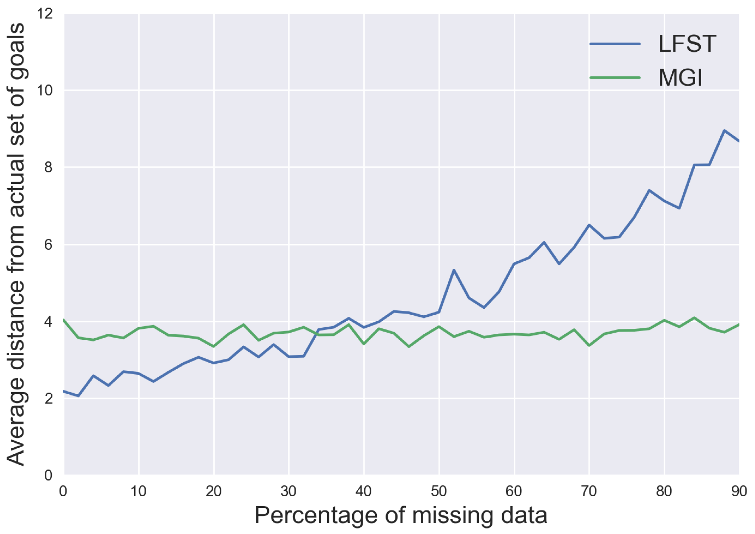
As shown by the experiment, the average syntactic distance between the agent’s actual goals and the results provided by LFST is pretty good because this average is a little less than 9 in the worst-case for GridWorld, as we can see in Figure 5. Knowing that for GridWorld, the agent has four goals composed of three atoms each, which means that on average, in the worst-case, LFST still finds almost one third of the atoms composing each real goal. Moreover, even when using as few as 20% of the initial data set, the results are still correct. Indeed, the average syntactic distance being around 5. It means that almost two thirds of the atoms composing each real goal of the agent are still deducted even in this case. MGI is more constant and thus stays to an average distance of 4 from the actual set of goals, being less precise than LFST until 60% of missing data where LFST gets worse. This difference can be explained by the fact that MGI will generate more specific prototypes than LFST. Thus, even if the actual goal is a conjunction of three atoms, MGI will generate a prototype of four or five atoms that cover the goal, and since they do not cover any negative examples, it will stop there. LFST will generate more general prototypes that the negative examples will invalidate, so the prototypes will start to be more and more specific and eventually as specific as the actual goals. Nevertheless, when there is not enough data, the prototypes which are too general will not be invalidated anymore due to the lack of negative examples, so the average syntactic distance from the actual goals will increase. However, as we can see in Figure 6, the accuracy of LFST is always better than the one of MGI and remains on average around $99.7\%$. As expected, the accuracy of both algorithms is decreasing with the quantity of data used. The difference between the two algorithms is that LFST will rarely fail to classify a positive example. Thus, it will produce very few False Negatives when MGI fails more often to classify a positive example. C4.5 has excellent accuracy in this environment, being even slightly better than LFST and reaching $100\%$ of accuracy, though it is only a small gain compare to LFST. However, the most significant difference in efficiency for the algorithms is the recall; Figure 7 shows that the value for the recall of LFST and C4.5 is much better than the one of MGI, which is just around the average ($50\%$). The reason for this result is the same as before since the recall is highly dependent on the number of False Negatives.

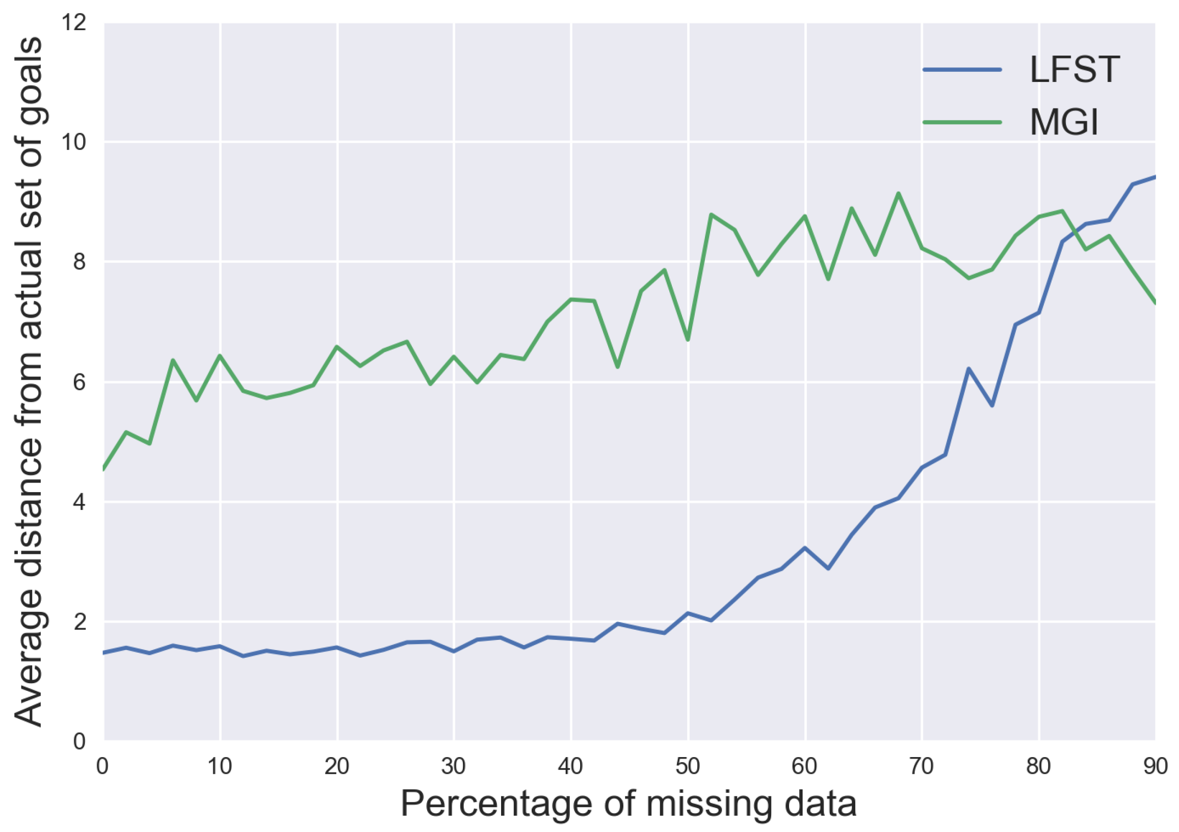
As for CubeWorld, in this environment, the agent has three goals of six atoms, so the syntactic distance cannot exceed 18, and we can see in Figure 8 that LFST obtains a bit less than 10 in the worst-case, so we infer more than one third of the goals in this case. The value of the distance for MGI is, on average, around 9, which is almost the worst value for LFST, so here also LFST is more accurate. The accuracy and the recall, Figure 9 and Figure 10 are also better here with LFST than with MGI, and here LFST also has better accuracy than C4.5, but it is a difference on the same scale as in the previous environment, relatively slight. The difference is more pronounced for the recall value, where LFST is also better than C4.5.

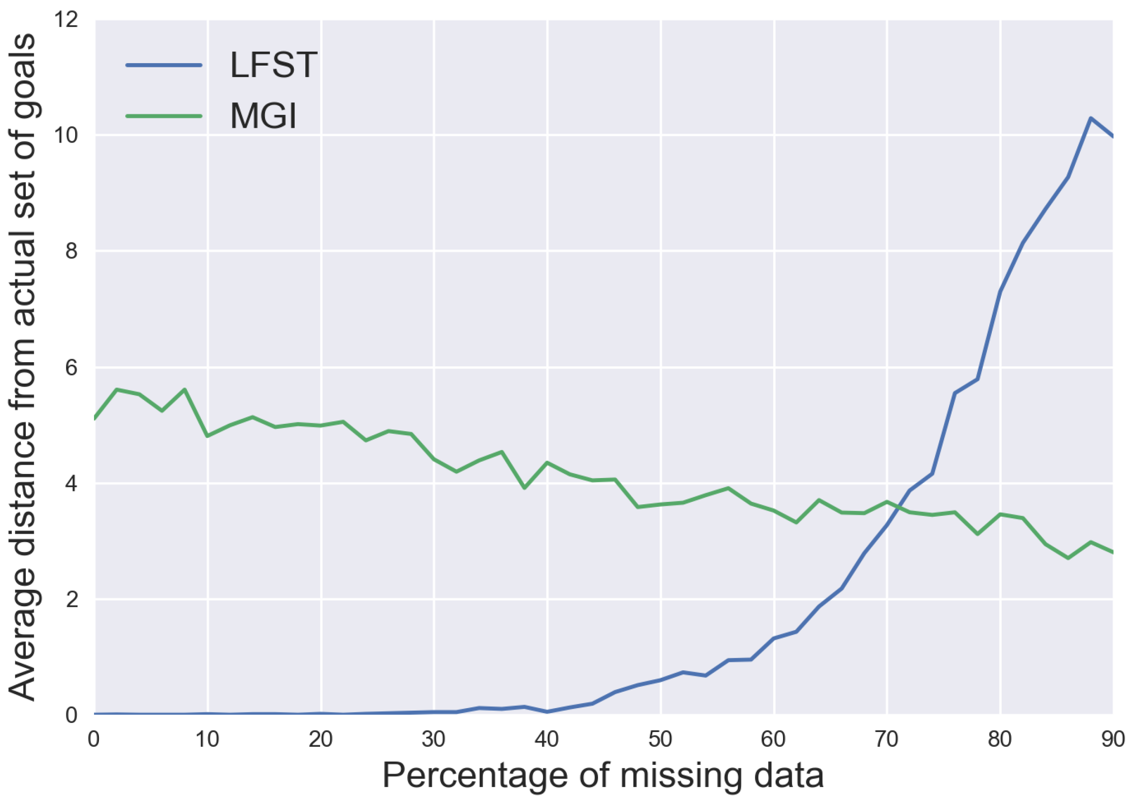
In 421World, since the agent’s goal is to obtain a dice combination of 421, the dice’s order and the fourth one’s value do not matter, which implies that there are many winning combinations, 24 to be exact. So, the agent has 24 goals that correspond to all the winning combinations. This environment is then the one that could potentially give the worst results. Though, as we can see in Figure 11 the syntactic distance from the actual goals is relatively low for both algorithms. The accuracy and recall Figure 12 and Figure 13 are less good than for the other environment, especially the recall for MGI is very low in this environment. We can observe a difference this time between LFST and C4.5, LFST being on average $10\%$ more accurate than C4.5.

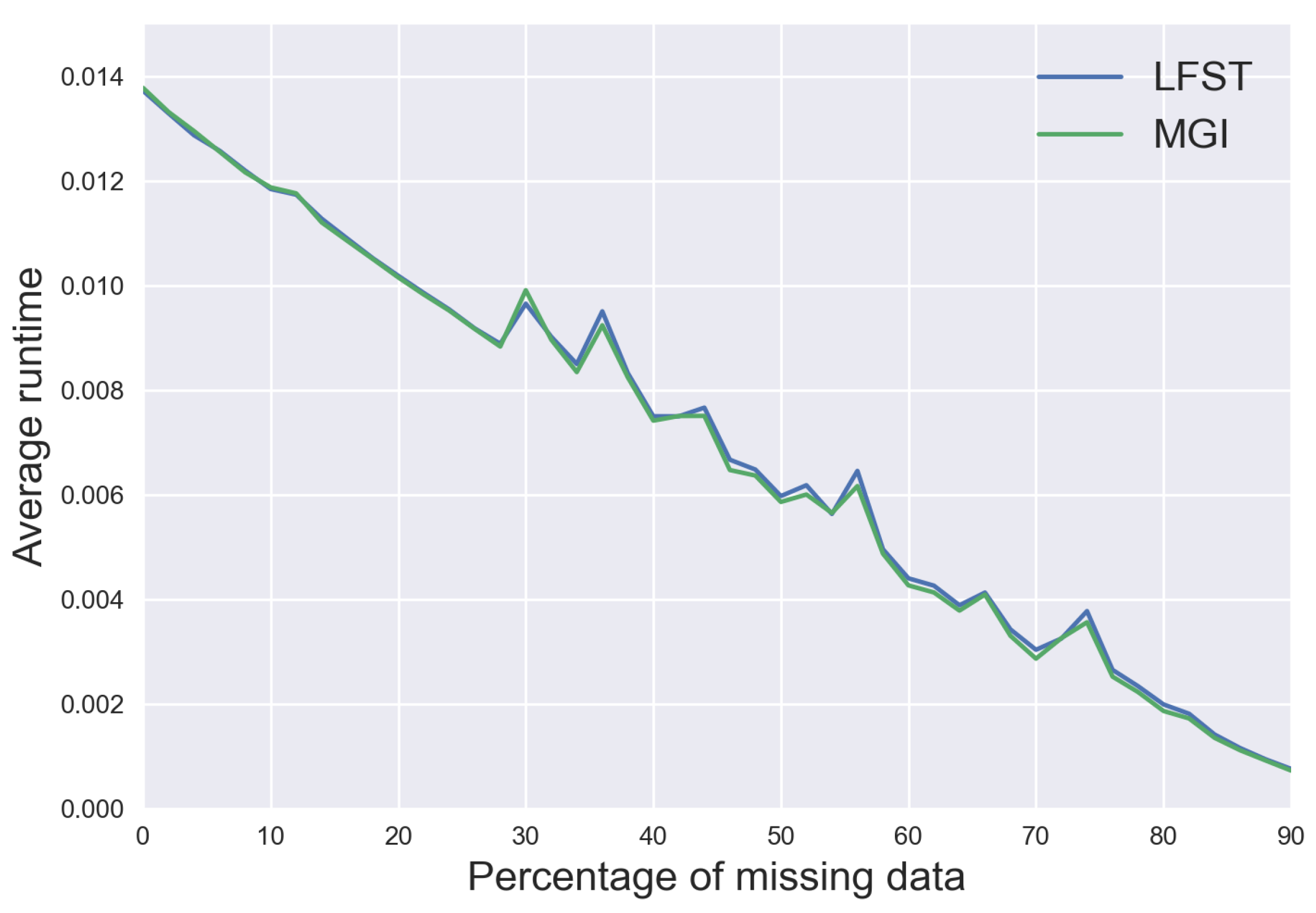
In these three environments, the performances of LFST are better than that of MGI. We also observe that LFST and C4.5 seem to have the same performances here, with a slight advantage for LFST, being better in two among three environments. Our guess was that C4.5 performs better in environments without a big difference between the number of positive and negative examples, though the results between CubeWorld and 421World do not necessarily validate this hypothesis. Nevertheless, that might be related to 421World itself that seems to be rather challenging for all the algorithms. However, if we must compare the algorithms’ running time when the number of variables to describe the environment increases. In that case, we can see a difference between LFST and MGI, as shown by Figure 14 and Figure 15, for GridWorld, there are five variables to describe the environment, and the two algorithms seems to be on the same order of computation time as the curves in Figure 14 are almost indistinguishable from each other. For CubeWorld, though, where we have 12 variables to describe the environment, MGI is faster than LFST; this can be seen in Figure 15, MGI is on average seven times faster than LFST. The difference between the execution time of both algorithms is because MGI uses a heuristic search to find the prototypes that will constitute the result when LFST does not. We chose CubeWorld and GridWorld to show these comparisons because one of the environments has the highest number of examples used as learning data, and the other the highest number of variables. We can see that for LFST, increasing the number of variables to describe the environment has a much more substantial impact on the computation time than increasing the number of examples, as it was expected according to the $O\left(\right|S_{positive}|\ast |S_{negative}|\ast 2^N)$ complexity of the algorithm. Still, the algorithm is pretty fast for these environments, and we could always play with the representation of the environment to avoid having a too high number of variables describing it. The experiments being done on an old CPU i7 two cores at 3.3GHz and using Python as the programming language. We cannot see C4.5 in Figure 14 and Figure 15, this is because C4.5 take much time compared to the two other algorithms to learn the concept (build the decision tree) 1.9 to 0.6 s on average for GridWorld and 1.5 to 0.5 s for CubeWorld, which makes it difficult to see the difference between MGI and LFST. One might argue that the learning time is not essential to learn concepts since it is just learned one time, though we believe that if it must be part of some real-time system, it is better to have a fast algorithm. We do think we made the right choice using our algorithm LFST for this problem since it performs as well if not better than traditional concept-learning algorithms, and compared to C4.5, LFST does produce the learning concept, thing that C4.5 is unable to do.

Table 1. Average accuracy and recall for the three algorithms in GridWorld.

	Accuracy			Recall
Percentage of Missing Data	LFST	C4.5	MGI	LFST	C4.5	MGI
0	99.85	99.99	98.51	100.0	100.0	44.1
4	99.83	99.99	98.39	100.0	100.0	41.04
8	99.82	99.99	98.36	100.0	100.0	41.3
12	99.84	99.99	98.38	100.0	100.0	43.52
16	99.83	99.98	98.29	100.0	100.0	41.82
20	99.81	99.98	98.19	100.0	100.0	40.43
24	99.78	99.96	98.24	100.0	100.0	43.68
28	99.78	99.97	98.13	100.0	100.0	42.22
32	99.79	99.98	98.11	100.0	100.0	43.0
36	99.78	99.98	98.0	100.0	100.0	42.18
40	99.75	99.98	97.88	100.0	100.0	40.63
44	99.74	99.96	97.88	99.93	100.0	42.41
48	99.7	99.96	97.78	99.94	100.0	41.57
52	99.69	99.96	97.64	100.0	100.0	40.41
56	99.73	99.93	97.58	99.94	100.0	40.87
60	99.6	99.92	97.5	99.79	100.0	41.88
64	99.54	99.93	97.45	99.42	99.79	42.73
68	99.53	99.87	97.25	98.51	99.67	41.88
72	99.47	99.88	97.17	97.38	99.56	42.16
76	99.36	99.8	96.95	95.95	99.25	42.68
80	98.91	99.63	97.0	92.23	98.26	44.2
84	98.48	99.31	96.69	85.36	96.36	48.11
88	97.73	98.87	96.36	77.58	93.37	47.67

,

Table 2. Average accuracy and recall for the three algorithms in CubeWorld.

	Accuracy			Recall
Percentage of Missing Data	LFST	C4.5	MGI	LFST	C4.5	MGI
0	100.0	98.5	89.7	100.0	98.51	21.99
4	100.0	98.35	89.69	100.0	98.19	21.94
8	100.0	98.38	89.49	100.0	98.48	21.51
12	100.0	98.09	89.3	100.0	97.62	21.79
16	99.98	98.07	89.1	100.0	97.13	22.98
20	99.98	97.9	89.21	99.86	96.53	23.83
24	100.0	97.9	89.34	100.0	96.16	22.82
28	99.98	97.69	89.07	100.0	96.1	23.18
32	99.96	97.76	89.03	99.89	96.44	26.25
36	99.98	97.72	89.17	100.0	95.37	27.09
40	99.95	97.62	89.18	99.8	95.78	25.19
44	99.95	97.43	89.22	100.0	94.39	28.0
48	99.85	97.38	89.04	99.49	94.47	26.4
52	99.85	97.21	88.83	99.22	93.26	27.1
56	99.72	97.04	89.22	99.03	93.71	29.26
60	99.46	96.49	89.17	97.19	92.56	30.87
64	99.27	96.53	89.27	96.55	91.89	31.99
68	99.03	96.43	88.68	94.9	91.25	34.17
72	98.6	96.21	88.5	92.55	91.44	31.85
76	98.22	96.09	89.85	88.59	91.31	37.58
80	96.89	95.57	89.75	81.5	88.41	43.17
84	95.72	94.27	89.75	73.29	85.21	46.87
88	93.78	93.63	89.89	62.33	84.17	50.08

and

Table 3. Average accuracy and recall for the three algorithms in 421World.

	Accuracy			Recall
Percentage of Missing Data	LFST	C4.5	MGI	LFST	C4.5	MGI
0	99.51	90.9	81.58	97.67	83.43	11.31
4	99.45	90.12	81.62	97.32	81.94	11.17
8	99.4	89.51	81.6	97.09	80.24	11.65
12	99.38	88.92	81.3	97.03	78.9	10.99
16	99.26	88.59	81.44	96.48	78.86	11.57
20	99.2	87.58	81.23	96.27	76.26	11.43
24	99.13	87.46	81.45	95.9	76.04	12.33
28	98.96	86.28	81.14	95.15	73.88	11.82
32	98.84	85.98	80.84	94.61	72.47	11.22
36	98.58	85.04	80.81	93.69	70.34	11.18
40	98.55	84.33	80.95	93.34	69.59	10.68
44	98.22	83.18	80.72	92.23	66.81	11.63
48	97.83	82.63	81.02	91.17	64.95	13.44
52	97.56	82.2	80.56	90.07	64.69	13.12
56	96.94	80.91	80.54	88.42	61.97	14.41
60	96.37	80.36	80.58	86.78	61.17	17.31
64	95.51	79.83	80.87	83.96	59.46	17.49
68	94.17	78.78	81.0	81.43	56.64	20.6
72	92.61	78.55	80.45	78.18	55.8	21.52
76	89.76	77.13	80.57	72.28	53.67	23.51
80	87.0	76.91	81.0	67.19	51.78	28.46
84	83.59	76.8	80.81	61.8	50.59	30.85
88	80.85	76.52	81.97	56.13	51.24	36.53

, are here to help the reader to visualize the accuracy and recall of the different algorithms on the three environments (only half of the data points have been included to reduce their size).

5. Inferring the Agent’s Model and Environment Rules from Data

In the previous sections, the input $\Sigma$, the set of successful traces, is simply reduced to two different sets of states $S_{negative}$ and $S_{positive}$. By doing so, we are not taking advantage of the information included in $\Sigma$ about the order in which the states are explored and the actions that the agent performs at each step. By ignoring these aspects, we have the advantage of being able to infer possible goals without more assumptions about the agent than the ones induced by successful traces how successful traces are defined, i.e., as soon as its goal is reached, the agent stops (with a success action) and this goal depends only on the current state of the environment. However, if the dynamics of the environment are known, it seems relevant to derive some information from what the agent has chosen to do, compared to what the agent could have done. It is only possible if we are given some insight into how the agent chooses its actions and takes decisions.

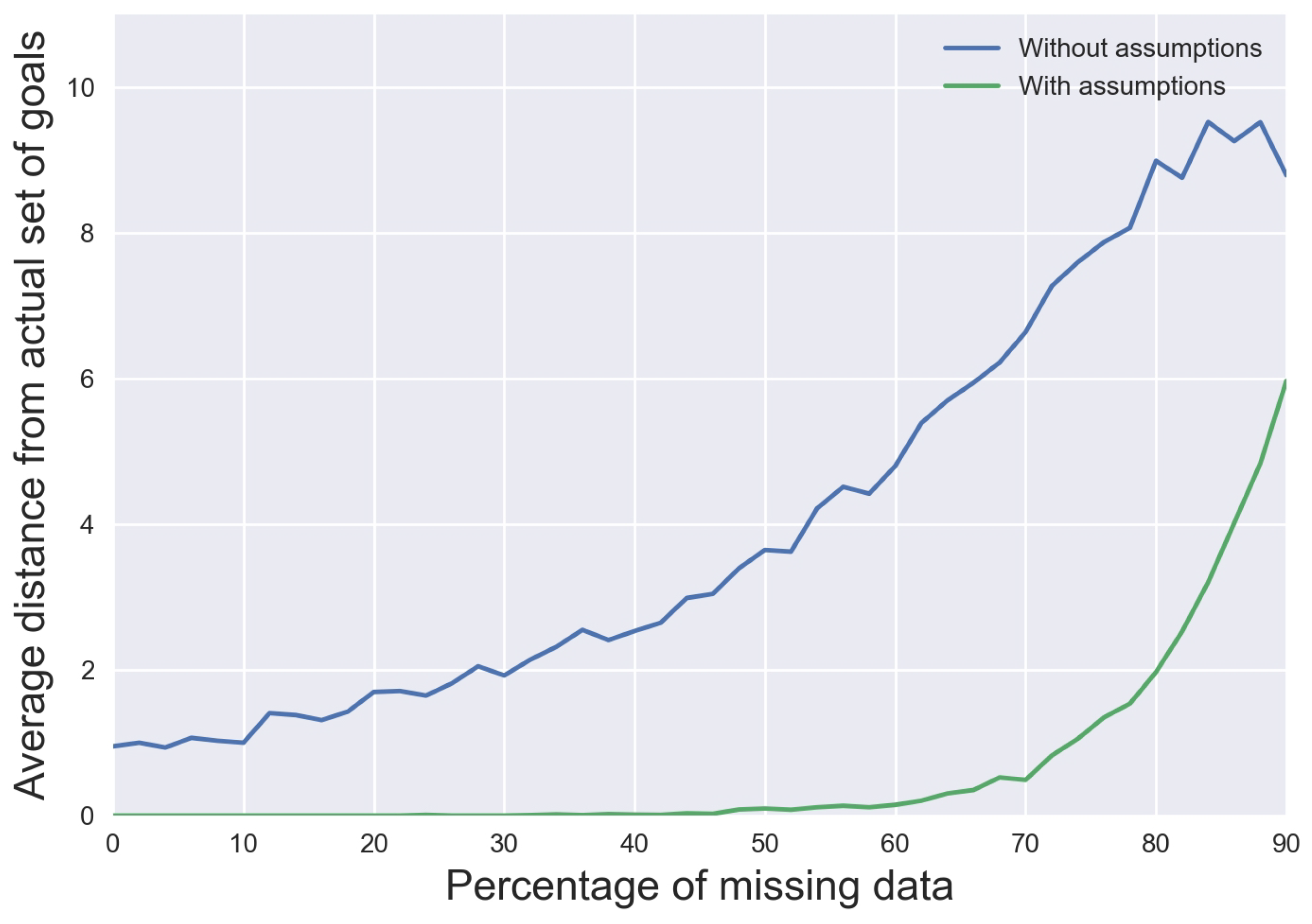
For instance, if we consider a rational omniscient agent’s case, we know that the observed agent has complete knowledge about its environment and its rules and uses a planner to compute the shortest plans to reach its goal. In such a case, by knowing the environment dynamics, we can use it to generate more negative examples, for each successful trace $T\in \Sigma$ of size K, all the negative examples that are reachable from the state i in $K-i$ steps can be generated and added to the set $S_{negative}$. We can compute this using $K_i$ times the function $next$ with every possible action to get all the reachable states. Using the same process with weaker assumptions, we consider now the case of a deterministic environment for which it is assumed that the agent is smart enough to reach its goal with only one move when its goal is reachable in one move (it cannot fail since the environment is deterministic). This amounts to considering that the agent can plan at least one step ahead, i.e., to understand its actions’ direct consequences and choose its actions accordingly. In such a case, when also knowing the environment and its dynamics, many negative examples can be generated. Indeed, if the action model ruling the effect of the agent’s actions is known, we can deduce from each state of the world the states that can be reached by the agent at the next time step. Next, if we know that at the time step t the agent did not reach its goal, it means that all the states that were reachable by the agent at the time step $t-1$ are not final ones. Furthermore, all these intermediate states can thus be regarded as negative examples, allowing us to refine the results of LFST by using more learning examples. In such a case, we modify LFST by this pre-processing that is applied to each $T\in \Sigma$ to compute additional negative examples. This process improves learning by expanding the initial input. It allows us to learn precise goals when using fewer original examples.

Figure 16 shows us the advantage of having these kinds of assumptions about the agent and environment. For this graph, the same experimental protocol as GridWorld is used but this time with a grid of size 4 × 4, which means that we have 192 positive examples and 776 negative ones that are used as input to LFST when no assumptions about the agent and environment are made. Then, we make two assumptions about the agent: the agent action model is known, and the agent can plan at least one step ahead so if its goal is reachable at step $t-1$, at step t it will reach it. These are not strong assumptions, and they allow us to generate more data from the 192 itineraries that have been followed by the agent throughout the simulation. In total, we get 2074 negative examples thanks to this data generation, which is almost three times more than what we have without making assumptions about the agent. We can see in Figure 16 that, as we expected, it allows LFST to generate more precise hypotheses about the agent’s goals since the result is much closer to the actual goals than when we do not make assumptions. As we can see in Figure 16, it allows us to be closer to the actual goals than when we use no assumptions. With enough knowledge about the agent’s action model, we can use the method of [12]. This method matches our method quite well since it needs a set of goals to find which ones are the more likely to be sought by the agent by using planning. So, we can first generate this set of goals by using LFST and then refine our set of possible goals with [12]. That allows us to correct some goals that could have been wrongly inferred by LFST. However, the combination of these two methods is not trivial. Indeed, the definition of a “goal” is not exactly the same between LFST and [12] since they define a goal as a final state where we define it as a conjunction of atoms which is included in this final state. It means that to check the validity of a goal generated by LFST, we need to go through all the traces where this specific conjunction appears in the description of a state of the world assume that in these traces, this state is a final state and then apply [12].

6. Discussion and Future Work

We have two interesting methods that we wish to exploit to deduce the agent’s action model and the environment rules. The first one is to use LFIT [35] which is a framework for learning normal logic programs from transitions of interpretations, which means that since we use a logical representation of the world, we will be able to infer the possible action model of the agent and the rules of the environment. In fact, to use LFIT, we just need a trace of the evolution of the states of the world in chronological order, which are the same data that we use to infer the agent’s goals. It means that we do not need an important modification of the data collection process to incorporate LFIT into our method, which is a good point. After processing these data with LFIT, we will obtain a set of rules that correspond to the possible transition from a state of the world to another. We will then have for each state of the world (observed previously in the collected data) the different actions that the agent did when it was in this state and the states of the world that it reached after these actions. So, we can infer a potential action model of the agent and the dynamic of the environment based on the observed transitions. Unfortunately, LFIT is not very robust against the lack of data, and the noise, especially the data need to cover as many transitions as possible between all the different possible states of the world. It is not very convenient because usually, the agent we observe is not acting randomly, and so, many possible transitions will never be observed. We also plan to use SMILE [36] another method that we can use to learn the action model of the agent. This method uses the same kind of data as LFIT, so here also the modification of the data collection process to use SMILE, and our method is not too cumbersome. Even if SMILE is usually used for a multi-agent system because it is, in fact, the different agents who will learn information about the other agents of the system, we can just create an agent “Observer” who will learn the action model of the observed agent. SMILE is more robust to the lack of data than LFIT but not as effective in some cases. So, we will choose which method to use based on the quantity of data obtained during the observation phase. We already tried SMILE and LFIT with our data to extract the agent’s action model and the rules of the environment. We obtained promising results, and so, we want to continue in this way. Nevertheless, we do not have combined our method and these two algorithms yet.

To improve our method and provide some more interesting hypotheses about the agents’ goals, we thought about incorporating a preferences function about these ones’ goals. It means that our hypothesis will provide us with a set of possible goals for an agent and ordered these goals according to the agent’s preferences. We want to start first with a simple preference model; by simple, we mean that if the agent prefers to reach the goal A rather than the goal B, its preferences will not consider the difficulty to reach these two goals. The process of inferring agents’ preferences will take place after the goals inference in our method. Because, of course, we need to know the agents’ goals to be able to order them. So, once we have the agent’s goals, we also need to know the agent’s action model, then, for each intermediate state of the trace of the agent, we can see if there are other reachable goals that the one reached in the final state of the trace and if so, compare the number of time that a goal was preferred to another one. If between two goals, one has always been preferred, and if it happened several times, we can assume a strict preference between them $A>B$. Otherwise, the preference will be more moderate $A⪰B$. Given an order of priority ${>}_p$ about an agent’s goals, we can translate the fact $A{>}_{p}B$ in a logic formula by assuming that if the agent finally reaches the goal B, it is because the goal A was not reachable. Then we can translate this in the logic formula $A\vee \neg A\wedge B$ (where A and B are atoms conjunctions) by using our language $\mathcal{L}$ described in Section 2. Likewise, if we have the preference $A{>}_{p}B{>}_{p}C$ on the agent’s goals we can write this $A\vee \neg A\wedge B\vee \neg A\wedge \neg B\wedge C$. With such a translation, we could write all the possible strict orders of preference on the agent’s goals, and since the writing still represents a DNF, we can modify a bit our algorithm and return a disjunction of such DNF as a result and thus obtain the possible goals of the agent and its preferences for these goals. If the agent is assumed rational, then such a simple linear model should work as transitivity (if $A{>}_{p}B$ and $B{>}_{p}C$ then $A{>}_{p}C$), antisymmetry ( if $A{>}_{p}B$ and $B{>}_{p}A$ then $A=B$) and connexity ($\forall A,B$ we have $A{>}_{p}B$ or $B{>}_{p}A$) should be supported by the agent’s preference model. Also, it could be hard to observe connexity, so we could have several partial orders instead. However, suppose the agent’s preferences are not rational (like a human, for example). In that case, this linear model will not work anymore, especially in human case the transitivity of preference is not always true, as shown by the “Condorcet paradox” or “voting paradox”, which is that when voting, majorities prefer, for example, candidate A over B, B over C, and yet C over A. If no cycles about the preference have been observed in the data, we can still assume that we have several partial orders; each of them could be represented as a DNF as described before. We still get a disjunction of DNF where goals will be ordered in their respective partial order (DNF), and the different partial orders could not be compared. Please note that if the goals A and B are not in relation but we have $A{>}_{p}C$ and $B{>}_{p}C$, we could write it $A\vee B\vee \neg A\wedge \neg B\wedge C$. We can start to work on this extension before completing the one in the previous section. Even if we need the agent’s action model, we can still assume that we know it and start the experiments such as this.

With our formalization, we do not take into account the cost of the actions for the agent and thus the fact that some goals could be achieved more often than others. If all the goals are achieved at least once, then our method should be able to infer them or build a hypothesis covering the state of the world corresponding to these goals. However, if one particular goal is never reached by the agent (because of its cost, for instance) during the observation process, it will be impossible to infer it with our current method as it is pretty challenging to learn from what has not been observed, especially if there is an important number of possible states of the world. We could potentially deal with this problem using a higher-level representation of the goals that we inferred once our first hypothesis was generated by LFST. A representation that could allow us to create a global concept for similar goals, and then we can look for states of the world covered by this concept and are not find in the set of negative examples used for learning. For instance, taking the case of GridWorld experiments, we saw that there are four possible dead ends. Let say that one of them was never reached by the agent, but LFST infer the three other kinds of dead ends as possible goals. When looking at the hypothesis returned by LFST, we could create the concept “dead-end”, which is that the agent is surrounded by three walls. We then check that there are no negative examples that reject this concept and keep it if it is not rejected. The concept “dead-end” will then cover even the fourth kind of dead-end that the agent did not reach when we were observing it. It could help us dealing with unobserved goals, but it needs human assistance or a way to generate concepts from a low-level representation of the environment.

Finally, the experiments’ results have shown that the main weakness of LFST is the execution time. We plan to improve the search for new potential goals since our method is currently quite exhaustive. A heuristic research method, as used for MGI, could significantly improve the execution time. However, the difficulty is then to find a good heuristic function. The clues that we have about the agent’s goals at the beginning are mainly in the positive examples set $S_{positive}$, then it will not be irrelevant to focus our attention on it. We want to use our syntactic distance to cluster these positives examples and group together those with a minimum distance from each other. Then we need to find the best way to construct a prototype that will cover all the positive examples within its cluster. It is not trivial, and we are currently working on it.

7. Conclusions

Goal Recognition has a broad variety of applications. Unfortunately, there are still several serious problems that slow down the use of goal recognition in large-scale real-world situations (computation time, action space, etc…). Moreover, a problem related to uncertainty, which is that in reality, it can be hard to know when an agent reaches its goal, but we will come back on this problem later. We reminded our method and showed how different it is from previous approaches in the field of goal recognition. Because few approaches are focused on learning the agent’s set of goals, they often consider it given in the problem. Moreover, our formalization of the problem also allows us to use concept learning. We use our algorithm, LFST, to control some generalization bias, and we have shown that it was a legitimate choice in Section 4 since our algorithm performs better than MGI and even C4.5. We could also make a version with a heuristic search of the prototype to improve the execution of LFST since it is the only point where MGI is better than LFST. We also showed that we could drastically improve the goals deduction process’s efficiency by making assumptions about the agent and its environment. Therefore, we plan to use LFIT or SMILE to infer the agents’ models and the environment’s rules to exploit such assumptions. This and the integration of the agents’ goals preferences in our model will allow us to infer more refined hypotheses about the agent’s goals. Also, as we said in Section 5 if we have good knowledge about the agent and its environment, we can combine our method to this one [12], and we might obtain rather promising results. We discussed the fact that in reality, it is hard to know when an agent reaches its goal. It is actually the main weakness of our method, and we need to overcome this weakness. For this, dynamic learning throughout the agent’s actions could be efficient and would be more realistic. It could also be effective in the case of an agent that changes its goal along the way or in a case where the agent repeats the same cycle of actions, cases that we cannot solve yet with our method.