
Wildlife Monitoring Using a Multi-UAV System with Optimal Transport Theory


Abstract
1. Introduction
2. Problem Description and Theoretical Background
- Wasserstein distance:
- Linear Programming problem: (for )
3. Method
3.1. Animal Movement Modeling
- Group center movement model (CRW):
- Individual animal movement model (BRW):
3.2. OT-Based Multi-UAV Exploration: Time-Invariant Case
3.2.1. A Three-Stage Approach
- Next goal point () determination stage:
- Weight update stage:
- Weight information exchange and update stage:
3.2.2. Algorithm
| Algorithm 1 Multi-Agent Exploration Algorithm |
|
3.3. Sample Point Generation and Propagation: Time-Varying Case
3.4. Other Exploration Strategy: Lawn Mower Method
4. Simulation Results
4.1. Unicycle Robot Dynamics
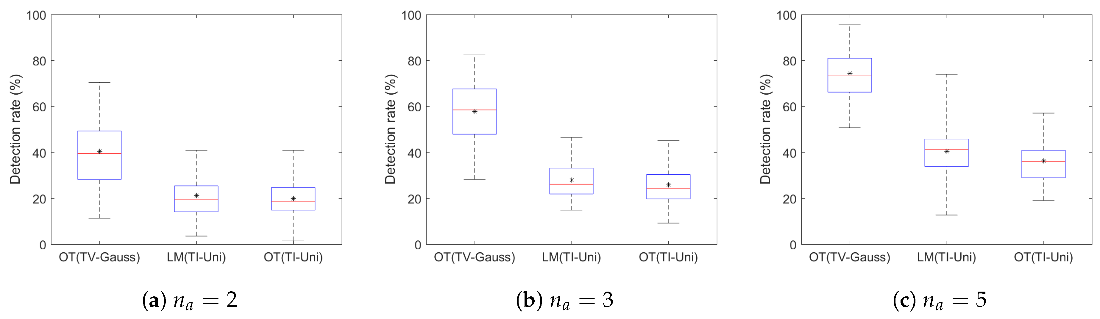
4.2. Variation in the Number of Agents
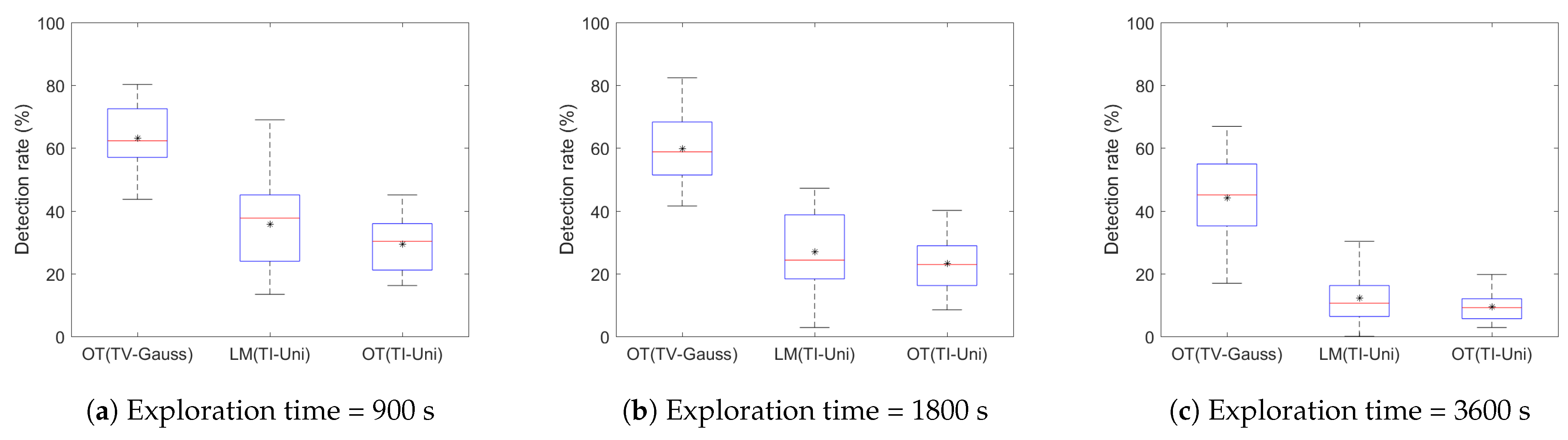
4.3. Variation in Exploration Time
5. Conclusions
Author Contributions
Funding
Institutional Review Board Statement
Informed Consent Statement
Data Availability Statement
Conflicts of Interest
References
- Tilman, D.; Clark, M.; Williams, D.R.; Kimmel, K.; Polasky, S.; Packer, C. Future threats to biodiversity and pathways to their prevention. Nature 2017, 546, 73–81. [Google Scholar] [CrossRef]
- Gardner, T.A.; Barlow, J.; Araujo, I.S.; Ávila-Pires, T.C.; Bonaldo, A.B.; Costa, J.E.; Esposito, M.C.; Ferreira, L.V.; Hawes, J.; Hernandez, M.I.; et al. The cost-effectiveness of biodiversity surveys in tropical forests. Ecol. Lett. 2008, 11, 139–150. [Google Scholar] [CrossRef]
- Meijaard, E.; Wich, S.; Ancrenaz, M.; Marshall, A.J. Not by science alone: Why orangutan conservationists must think outside the box. Ann. N. Y. Acad. Sci. 2012, 1249, 29–44. [Google Scholar] [CrossRef] [PubMed]
- Palace, M.; Keller, M.; Asner, G.P.; Hagen, S.; Braswell, B. Amazon forest structure from IKONOS satellite data and the automated characterization of forest canopy properties. Biotropica 2008, 40, 141–150. [Google Scholar] [CrossRef]
- Stapleton, S.; LaRue, M.; Lecomte, N.; Atkinson, S.; Garshelis, D.; Porter, C.; Atwood, T. Polar bears from space: Assessing satellite imagery as a tool to track Arctic wildlife. PLoS ONE 2014, 9, e101513. [Google Scholar] [CrossRef]
- Mammals Program, Colorado Division of Wildlife. Year: July 2003–June 2004. Available online: https://spl.cde.state.co.us/artemis/nrserials/nr616internet/nr616200304internet.pdf (accessed on 15 March 2021).
- Zimmermann, F.; Foresti, D.; Rovero, F. Behavioural studies. Camera Trapping for Wildlife Research; Pelagic Publishing Ltd.: Exeter, UK, 2016; pp. 142–167. [Google Scholar]
- Murphy, A.J.; Goodman, S.M.; Farris, Z.J.; Karpanty, S.M.; Andrianjakarivelo, V.; Kelly, M.J. Landscape trends in small mammal occupancy in the Makira–Masoala protected areas, northeastern Madagascar. J. Mammal. 2017, 98, 272–282. [Google Scholar] [CrossRef]
- Alvarez-Berríos, N.; Campos-Cerqueira, M.; Hernández-Serna, A.; Amanda Delgado, C.; Román-Dañobeytia, F.; Aide, T.M. Impacts of small-scale gold mining on birds and anurans near the Tambopata Natural Reserve, Peru, assessed using passive acoustic monitoring. Trop. Conserv. Sci. 2016, 9, 832–851. [Google Scholar] [CrossRef]
- Deichmann, J.L.; Hernandez-Serna, A.; Campos-Cerqueira, M.; Aide, T.M. Soundscape analysis and acoustic monitoring document impacts of natural gas exploration on biodiversity in a tropical forest. Ecol. Indic. 2017, 74, 39–48. [Google Scholar] [CrossRef]
- Biggs, J.; Ewald, N.; Valentini, A.; Gaboriaud, C.; Dejean, T.; Griffiths, R.A.; Foster, J.; Wilkinson, J.W.; Arnell, A.; Brotherton, P.; et al. Using eDNA to develop a national citizen science-based monitoring programme for the great crested newt (Triturus cristatus). Biol. Conserv. 2015, 183, 19–28. [Google Scholar] [CrossRef]
- Valentini, A.; Taberlet, P.; Miaud, C.; Civade, R.; Herder, J.; Thomsen, P.F.; Bellemain, E.; Besnard, A.; Coissac, E.; Boyer, F.; et al. Next-generation monitoring of aquatic biodiversity using environmental DNA metabarcoding. Mol. Ecol. 2016, 25, 929–942. [Google Scholar] [CrossRef] [PubMed]
- Gray, M.; Roy, J.; Vigilant, L.; Fawcett, K.; Basabose, A.; Cranfield, M.; Uwingeli, P.; Mburanumwe, I.; Kagoda, E.; Robbins, M.M. Genetic census reveals increased but uneven growth of a critically endangered mountain gorilla population. Biol. Conserv. 2013, 158, 230–238. [Google Scholar] [CrossRef]
- Zanol, R.; Chiariotti, F.; Zanella, A. Drone mapping through multi-agent reinforcement learning. In Proceedings of the 2019 IEEE Wireless Communications and Networking Conference (WCNC), Marrakesh, Morocco, 15–18 April 2019; pp. 1–7. [Google Scholar]
- Li, X.; Huang, H.; Savkin, A.V. Use of A UAV Base Station for Searching and Bio-inspired Covert Video Surveillance of Tagged Wild Animals. In Proceedings of the 2020 IEEE Australian and New Zealand Control Conference (ANZCC), Gold Coast, QLD, Australia, 26–27 November 2020; pp. 87–90. [Google Scholar]
- Kellenberger, B.; Volpi, M.; Tuia, D. Fast animal detection in UAV images using convolutional neural networks. In Proceedings of the 2017 IEEE International Geoscience and Remote Sensing Symposium (IGARSS), Fort Worth, TX, USA, 23–28 July 2017; pp. 866–869. [Google Scholar]
- Caballero, L.C.; Saito, C.; Micheline, R.B.; Paredes, J.A. On the design of an UAV-based store and forward transport network for wildlife inventory in the western Amazon rainforest. In Proceedings of the 2017 IEEE XXIV International Conference on Electronics, Electrical Engineering and Computing (INTERCON), Cusco, Peru, 15–18 August 2017; pp. 1–4. [Google Scholar]
- Valavanis, K.P.; Vachtsevanos, G.J. Handbook of Unmanned Aerial Vehicles; Springer: Berlin/Heidelberg, Germany, 2015; Volume 1. [Google Scholar]
- Zeng, Y.; Wu, Q.; Zhang, R. Accessing from the sky: A tutorial on UAV communications for 5G and beyond. Proc. IEEE 2019, 107, 2327–2375. [Google Scholar] [CrossRef]
- Dufour, S.; Bernez, I.; Betbeder, J.; Corgne, S.; Hubert-Moy, L.; Nabucet, J.; Rapinel, S.; Sawtschuk, J.; Trollé, C. Monitoring restored riparian vegetation: How can recent developments in remote sensing sciences help? Knowl. Manag. Aquat. Ecosyst. 2013, 410, 10. [Google Scholar] [CrossRef]
- Evans, I.; Jones, T.H.; Pang, K.; Evans, M.N.; Saimin, S.; Goossens, B. Use of drone technology as a tool for behavioral research: A case study of crocodilian nesting. Herpetol. Conserv. Biol. 2015, 10, 90–98. [Google Scholar]
- Ivosevic, B.; Han, Y.G.; Cho, Y.; Kwon, O. The use of conservation drones in ecology and wildlife research. J. Ecol. Environ. 2015, 38, 113–118. [Google Scholar] [CrossRef]
- Lorah, P.; Ready, A.; Rinn, E. Using drones to generate new data for conservation insights. Int. J. Geospat. Environ. Res. 2018, 5, 2. [Google Scholar]
- Lu, B.; He, Y. Species classification using Unmanned Aerial Vehicle (UAV)-acquired high spatial resolution imagery in a heterogeneous grassland. ISPRS J. Photogramm. Remote Sens. 2017, 128, 73–85. [Google Scholar] [CrossRef]
- Chabot, D.; Bird, D.M. Wildlife research and management methods in the 21st century: Where do unmanned aircraft fit in? J. Unmanned Veh. Syst. 2015, 3, 137–155. [Google Scholar] [CrossRef]
- Koh, L.P.; Wich, S.A. Dawn of drone ecology: Low-cost autonomous aerial vehicles for conservation. Trop. Conserv. Sci. 2012, 5, 121–132. [Google Scholar] [CrossRef]
- Linchant, J.; Lisein, J.; Semeki, J.; Lejeune, P.; Vermeulen, C. Are unmanned aircraft systems (UAS s) the future of wildlife monitoring? A review of accomplishments and challenges. Mammal Rev. 2015, 45, 239–252. [Google Scholar] [CrossRef]
- Villani, C. Optimal Transport: Old and New; Springer Science & Business Media: Berlin/Heidelberg, Germany, 2008; Volume 338. [Google Scholar]
- Lee, K.; Halder, A.; Bhattacharya, R. Probabilistic robustness analysis of stochastic jump linear systems. In Proceedings of the 2014 IEEE American Control Conference (ACC), Portland, OR, USA, 4–6 June 2014; pp. 2638–2643. [Google Scholar]
- Lee, K.; Halder, A.; Bhattacharya, R. Performance and robustness analysis of stochastic jump linear systems using wasserstein metric. Automatica 2015, 51, 341–347. [Google Scholar] [CrossRef]
- Lee, K. Analysis of Large-Scale Asynchronous Switched Dynamical Systems. Ph.D. Thesis, Texas A & M University, College Station, TX, USA, 2015. [Google Scholar]
- Lee, K.; Bhattacharya, R. Optimal switching synthesis for jump linear systems with gaussian initial state uncertainty. In Proceedings of the ASME 2014 Dynamic Systems and Control Conference, San Antonio, TX, USA, 22–24 October 2014; American Society of Mechanical Engineers: San Antonio, TX, USA, 2014; p. V002T24A003. [Google Scholar]
- Lee, K.; Bhattacharya, R. Optimal controller switching for resource-constrained dynamical systems. Int. J. Control. Autom. Syst. 2018, 16, 1323–1331. [Google Scholar] [CrossRef]
- Bovet, P.; Benhamou, S. Spatial analysis of animals’ movements using a correlated random walk model. J. Theor. Biol. 1988, 131, 419–433. [Google Scholar] [CrossRef]
- Bergman, C.M.; Schaefer, J.A.; Luttich, S. Caribou movement as a correlated random walk. Oecologia 2000, 123, 364–374. [Google Scholar] [CrossRef]
- Halstead, B.J.; McCoy, E.D.; Stilson, T.A.; Mushinsky, H.R. Alternative foraging tactics of juvenile gopher tortoises (Gopherus polyphemus) examined using correlated random walk models. Herpetologica 2007, 63, 472–481. [Google Scholar] [CrossRef]
- Kadota, M.; Torisawa, S.; Takagi, T.; Komeyama, K. Analysis of juvenile tuna movements as correlated random walk. Fish. Sci. 2011, 77, 993–998. [Google Scholar] [CrossRef]
- Kareiva, P.; Shigesada, N. Analyzing insect movement as a correlated random walk. Oecologia 1983, 56, 234–238. [Google Scholar] [CrossRef] [PubMed]
- Langrock, R.; Hopcraft, J.G.C.; Blackwell, P.G.; Goodall, V.; King, R.; Niu, M.; Patterson, T.A.; Pedersen, M.W.; Skarin, A.; Schick, R.S. Modelling group dynamic animal movement. Methods Ecol. Evol. 2014, 5, 190–199. [Google Scholar] [CrossRef]


| Parameters | Parameter Values | |||
|---|---|---|---|---|
| Exploration strategies | 3 (OT (TV-Gauss), LM (TI-Uni), OT (TI-Uni)) | |||
| No. of agents | 2, 3, 5 (for each strategy) | |||
| No. of simulations | 30 (for each strategy with a specific no. of agents) | |||
| Exploration time | 900 s | |||
| Time delay | 600 s | |||
| No. of animal herds | 9 | |||
| Initial locations (m) of the animal herds and populations in each herd | 1: , 2: | |||
| 3: , 4: | ||||
| 5: , 6: | ||||
| 7: , 8: | ||||
| 9: | ||||
| Initial GPS tracker information for 9 tracked animals (m) | 1: , 2: | |||
| 3: , 4: | ||||
| 5: , 6: | ||||
| 7: , 8: | ||||
| 9: | ||||
| Estimated herd center (m) from Section 3.3 with tracked animal no. | 1: , 3,4,9, 2: , 5 | |||
| 3: , 1, 4: , 7 | ||||
| 5: , 2,8, 6: , 6 | ||||
| Distribution parameters for animalherd movement | m/s, m/s) | |||
| , | ||||
| , | ||||
| , | ||||
| Exploration domain size | 2500 m × 3000 m | |||
| Maximum velocity of the UAVs | 30 m/s | |||
| Minimum velocity of the UAVs | 10 m/s | |||
| Angular velocity limit | 30 | |||
| Positional error gain, | ||||
| Angular error gain, | 1 | |||
| UAV sensor range to detect animals, | 15 m | |||
| Specific parameters for OT (TV-Gauss) | Number of sample points, N | 3600 | ||
| Number of UAV steps for each agent for exploration, | 900 | |||
| Initial covariance for the sample point clusters | ||||
| Herd threshold | 50 m | |||
| Horizon length, h | 5 | |||
| Search radius, r | 0.1 m | |||
| Radius increment, | 0.05 m | |||
| Initial robot positions | [100 m, 400 m] | |||
| [200 m, 600 m] | ||||
| [200 m, 150 m] | ||||
| [150 m, 400 m] | ||||
| [400 m, 750 m] | ||||
| Distribution parameters for the sample point propagation | = 0.6 m/s, = 0.05 m/s) | |||
| , | ||||
| = , | ||||
| Specific parameters for LM (TI-Uni) | Horizontal and vertical expansion factors, , | 1 | ||
| Distance between adjacent waypoints, | 10 m | |||
| Spacing between adjacent vertical lines | 120 m, 70 m, 40 m for , 3, 5, respectively | |||
| Simulation output | No. of UAVs | Average Detection Rate (%) | ||
| OT(TV-Gauss) | LM(TI-Uni) | OT(TI-Uni) | ||
| 2 | 40.45 | 21.08 | 19.86 | |
| 3 | 57.72 | 27.86 | 25.85 | |
| 5 | 74.34 | 40.31 | 36.22 | |
| Parameters | Parameter Values | |||
|---|---|---|---|---|
| Exploration strategies | 3 (OT (TV-Gauss), LM (TI-Uni), OT (TI-Uni)) | |||
| Exploration time | 900, 1800, 3600 s (for each strategy) | |||
| No. of UAVs | 3 | |||
| Time delay | 600 | |||
| No. of simulations | 30 (for each strategy with a specific exploration time | |||
| Initial UAV positions (m) (OT(TV-Gauss) and OT(TI-Uni)) | ||||
| Parameters varied with exploration time | Exploration Time | |||
| 900 | 1800 | 3600 | ||
| Exploration domain size(m2) | 2500 × 2500 | 3000 × 4000 | 7000 × 7000 | |
| Number of UAV steps for each agent for exploration, (OT(TV-Gauss)) | 900 | 1800 | 3600 | |
| Horizontal and vertical expansion factors, , (LM(TI-Uni)) | 1 | |||
| Spacing between adjacent vertical lines (LM(TI-Uni)) | 120 | 70 | 40 | |
| Simulation output | Exploration Strategy | Average Detection Rate (%) | ||
| 900 | 1800 | 3600 | ||
| OT (TV-Gauss) | 63.08 | 59.84 | 44.08 | |
| LM (TI-Uni) | 35.63 | 26.90 | 12.16 | |
| OT (TI-Uni) | 29.34 | 23.19 | 9.39 | |
Publisher’s Note: MDPI stays neutral with regard to jurisdictional claims in published maps and institutional affiliations. |
© 2021 by the authors. Licensee MDPI, Basel, Switzerland. This article is an open access article distributed under the terms and conditions of the Creative Commons Attribution (CC BY) license (https://creativecommons.org/licenses/by/4.0/).
Share and Cite
Kabir, R.H.; Lee, K. Wildlife Monitoring Using a Multi-UAV System with Optimal Transport Theory. Appl. Sci. 2021, 11, 4070. https://doi.org/10.3390/app11094070
Kabir RH, Lee K. Wildlife Monitoring Using a Multi-UAV System with Optimal Transport Theory. Applied Sciences. 2021; 11(9):4070. https://doi.org/10.3390/app11094070
Chicago/Turabian StyleKabir, Rabiul Hasan, and Kooktae Lee. 2021. "Wildlife Monitoring Using a Multi-UAV System with Optimal Transport Theory" Applied Sciences 11, no. 9: 4070. https://doi.org/10.3390/app11094070
APA StyleKabir, R. H., & Lee, K. (2021). Wildlife Monitoring Using a Multi-UAV System with Optimal Transport Theory. Applied Sciences, 11(9), 4070. https://doi.org/10.3390/app11094070