Decision Tree Method for Fault Causes Classification Based on RMS-DWT Analysis in 275 kV Transmission Lines Network

Abstract

This paper presents a statistical algorithm for classification of fault causes on power transmission lines. The proposed algorithm is based upon the root mean square (RMS) current duration, voltage dip, and discrete wavelet transform (DWT) measured at the sending end of a line and the decision tree method, a commonly accessible measurable method. Fault duration of RMS current signal, voltage dip, and DWT gives concealed data of a fault signature as a contribution to decision tree calculation which is utilized to classify various fault causes. The proposed method was carried out in the MATLAB/SIMULINK programming platform based upon the information made with the fault analysis of the 275 kV sample transmission line considering wide variations in the operating conditions. The classifier performance of different parameters was also compared in a confusion matrix form to obtain the best classification results of the decision tree.

1. Introduction

Unplanned electrical power outages have become a major issue to a power utility [1,2]. A temporary loss of interruption of power source especially a loss of electric power might affect the economic and security issue. The outage that occurred due to an equipment tripping or failure is categorized as force outage. According to the IEEE std 524, the equipment failure also known as electrical fault is defined as a physical condition that causes a device, component, or an element to fail to perform in a required manner. Transmission line networks, which consist of overhead lines and cable lines are susceptible to various system faults. In order to address the issues brought by faults in the power system, identification of the root cause of faults by its signature is necessary. Acquiring knowledge of the outage’s cause immediately after the faults is highly helpful to reduce the outage’s duration [3]. Several studies have been carried out to identify the root cause of fault such as due to natural phenomenon, equipment failures, and human error. The most common fault caused in overhead transmission lines is due to natural phenomena such as lightning, wind, tree growth, and bushfire.

Among the tremendous root cause of fault are the several types of phenomenon that prominently occur in Malaysia’s transmission line system such as lightning, tree encroachment, crane encroachment, insulator degrading, and bushfire [4,5,6]. In most cases, the fault occurs and becomes a risk and would obviously reduce the productivity of the installation, in addition to the cost of maintenance to restore the system with normal conditions as well as the loss. To reduce the maintenance cost and increase the system availability and productivity at optimal performances, we proceed to early fault detection. It is possible to classify the faults by looking from different aspects, in particular: the fault current duration when it increases by a certain percentage, voltage dip percentage, and energy decomposition value. The classification tool works based on the acquired process parameters such as current signal, voltage signal, and frequency. The acquired signals of fault causes classification process contain the dynamic information about duration and voltage dip.

Regardless of which measure boundaries are chosen, signal processing techniques such as time domain, frequency domain, and time–frequency domain analyses a lot of signal features to anticipate various types of fault. Previously, many researchers proposed a signal processing method to detect and classify faults. Saravanan et al. [2] diagnosed the gear box fault using discrete wavelet transform (DWT) and classified the fault using artificial neural network (ANN). The ANN is capable of classifying the gear box fault on various conditions based on numerical values extracted from the wavelet energy decomposition. In [7], Malathy et al. proposed a continuous density hidden Markov model (CDHMM) to determine the dynamics of the state transition due to fault occurrences and classify the condition using neural networks. In addition, Sheng et al. proposed rotating machinery fault diagnosis using convolutional neural network (CNN) [8]. Fault detection using fuzzy method has also been proposed for photovoltaic (PV) protection [9]. Voltage ratio (VR) and power ratio (PR) are applied as input data for ANN to categorize fault regions in examining PV. Then, the second technique is implemented to detect the exact fault in the PV system. Centroid type for defuzzification process is chosen and 10 different membership functions are considered for fuzzy logic process. In [10], the author proposed fuzzy cause-and-effect network (FCE) in DS for fault diagnosis. The measurement of feeder currents and bus voltage derived from SCADA is converted into fuzzy terms before it is specified into the membership function of fuzzy sets. Furthermore, a decision tree is widely used for fault detection and classification [11]. Saravanan et al. proposed decision tree classify rules to build a repository of faults in a gear box based on statistical value extracted from wavelet transform [12]. Furthermore, Upendar et al. proposed the same method to classify the types of faults in 400 kV power transmission line networks and comparing the accuracy results with obtaining back-propagation neural network [13]. Rabah et al. implemented a decision tree to detect and diagnose the fault in grid connected photovoltaic systems under several weather conditions [14].

In much of the previous research, it is observed that the fault detection in overhead transmission lines is mainly focusing on the types of fault whether it is line-to-line fault or grounding fault. However, because of the diversity root cause of faults along the complex connection of transmission lines, it is difficult to identify the fault causes based on signal waveform recorded thus, less exploration made on previous study. In our proposed fault causes identification, we provide the fault signatures based on signal characterization to differentiate four types of fault causes which mainly occurred in Malaysian 275 kV overhead line system. In addition, the fault causes are further classified using decision tree technique since it gains a prudent accuracy and low cost computation among other signal processing techniques [11]. To extract useful information, RMS fault current duration, voltage dip, and DWT features are extracted and significant features are selected from raw signals using a decision tree. These criteria might be very informative for further analysis to identify any other fault causes such as bushfire, animal encroachment, and falling objects. An 840 sample set of signals are classified in a decision tree with different predictor selection to find the most accurate classifier with the best computation time.

2. Related Works

The analysis of fault signature involves four essential steps starting with collection of statistical and waveform data, fault characterization, develop fault algorithm model using simulation study and fault classification process. An overall step involved in the fault signature analysis is illustrated in Figure 1. In the first stage, the statistical fault data which has been endorsed by the committee meeting was obtained to identify their root cause. The utmost root cause of faults is sorting out to merge with their, system voltage involved, relative activities and time occurrences. Then, the voltage and current waveform are acquired and all the signatures of different fault causes are identified. In the fault characterization stage, fault current and voltage waveform chosen are converted to root mean square (RMS) waveform to establish their criteria. The behavior of each parameter is determined and evaluated. Since actual data is insufficient to be classified, several fault models regarding on the fault causes are developed in the MATLAB/SIMULINK environment. Several parameters such as fault distance, inception angle, and load are varied to study their effects on the fault signature. Then, the generated waveforms produced from the simulation are compared with the actual waveforms from the field to validate the results. Finally, the actual waveform and output waveform generated from the simulation are trained and tested in a decision tree tool for classification purposes. The decision tree will handle the numerical and categorical variables by ruling out features condition using the splitting method.

2.1. Parameters Condition

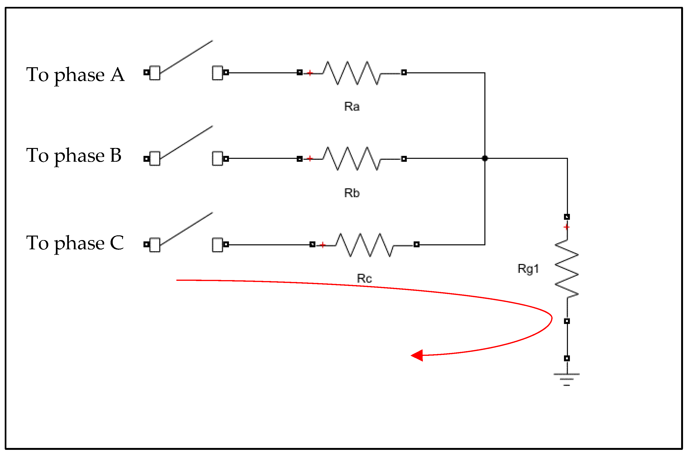
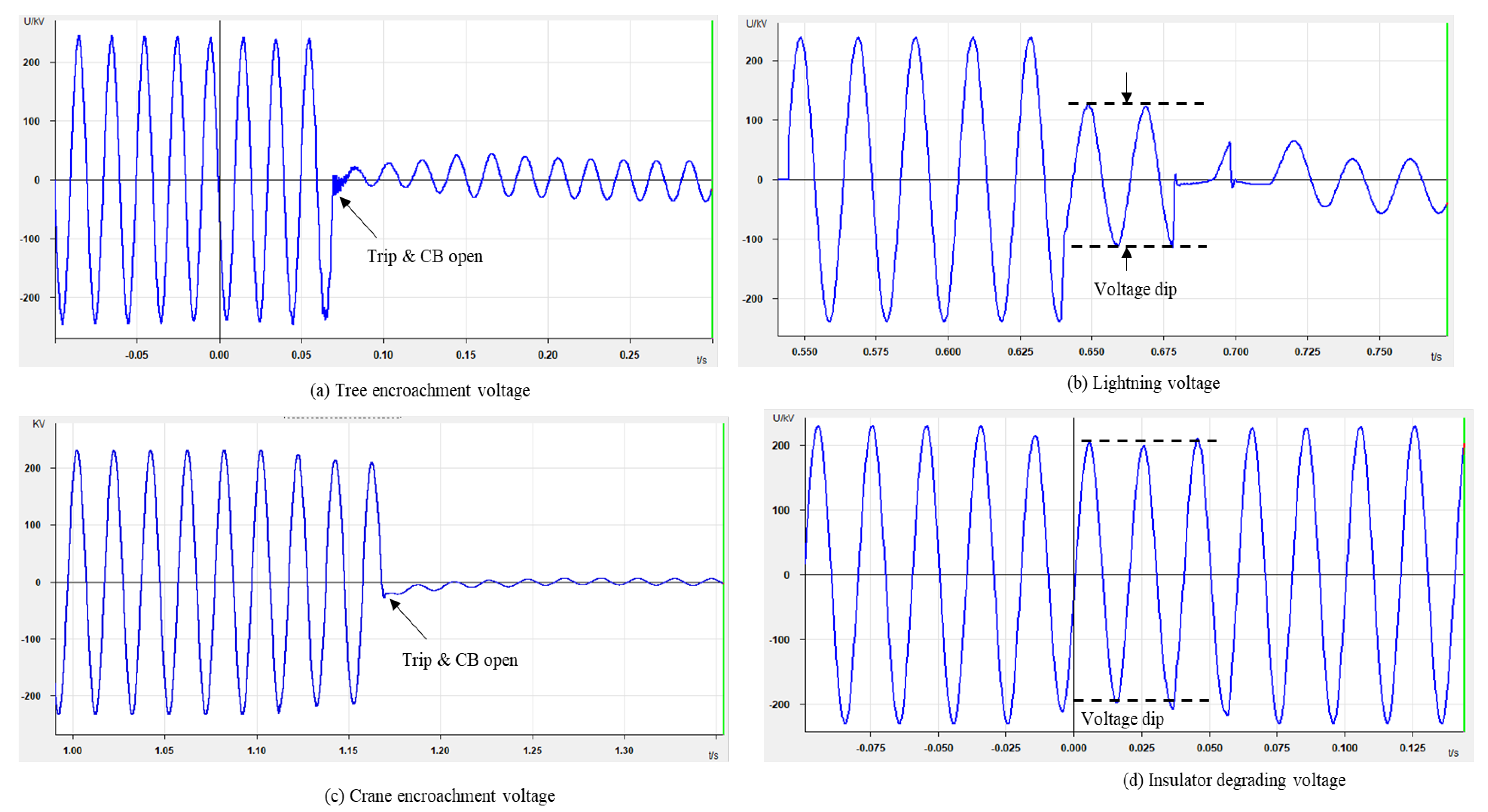
The transmission line has been modeled using the frequency-dependent phase model, which is the most accurate model, as it represents all frequency-dependent effects of a transmission line, and is very useful to study the fault behavior of the line. MATLAB-Simulink is used to generate four types of fault causes in three-phase transmission line system. In this model, the transmission line is connected with the same voltage level at the sending and receiving voltage source with 100 MVA, and 275 kV buses. The load is assumed to be connected at the end of receiving line before the measurement takes place. The current transformer model is implemented for measurement purposes where the grounding circuit is utilized in the system. The fault model has been connected to the transmission line with total length of 300 km line. The Simulink parameters of test system model are set as per

Table 1. Simulink parameters for the test system model.

Item	Value
Frequency (Hz)	50
Sample per cycle	100
Sampling time (s)	2 × 10−4
Run time (s)	0.2

.

Several parameters are varied to determine the effects on the fault signatures. The variable parameters are fault distance, fault inception angle, and load as described in

Table 2. Variable parameters set up in the simulation model.

Variable Parameters	Quantity
Fault distance (km)	10 to 100 (step size 10 km)
Phase angle (°)	0, 30, 45, 60, 90, 180, 270
Load (MW)	200, 300, 330

. The distance of fault is various from 10 km to 100 km from the receiving end where the total line length is equivalent to 300 km. The fault current and voltage waveform are measured after fault distance is varied after every 10 km. Meanwhile, fault inception angle is varied from 0°, 30°, 45, 60°, 90°, 180°, and 270°. Finally, load parameter using RL circuit is varied to be 300 MW, 330 MW, and 150 MW.

2.2. Fault Model

The following subsection explains the adopted model for fault causes used in the study.

2.2.1. Tree Fault Model

The dangers of a downed conductor are obvious to all. The possibility of fire, property damage, and anything that comes into contact with the live conductor are the major concerns where it produces arc and causes fault [15]. Tree and crane contact that cause fault are categorized under high impedance fault (HIF) where, in the HIF model used, the parameters Vp and Vn model the contact surfaces. During the HIF, current of positive half cycle value will be higher than the negative half cycle where the waveform is known as unsymmetrical and it was experimentally proven by Emanuel et al. Therefore, to model this phenomenon, Vn must be greater than Vp (Vn > Vp), and Vn − Vp = ΔV, where ΔV is unsymmetrical voltage. Moreover, it was shown that less densely packed contact surface yields a higher arc voltage than contact surface with high density. Using this as a guide, tree encroachment and crane are modeled to obtain the specified current magnitudes. Furthermore, the values for Rp and Rn parameters are randomly varied between +10% of the specified steady-state values and represent the effective fault resistance for positive and negative half cycles, respectively [16,17,18,19,20,21]. The HIF model based on Emanuel arc is shown in Figure 2. The equations involved in these algorithms are derived in Equations (1)–(4).

Therefore, the fault resistance for tree cause can be defined as:

$$R_{Ftr}=\frac{R_P{R}_N}{R_p+R_N}$$

(1)

Parallel of total $R_{FCtr}$ in Emanuel arc can be defined as:

$$R_{FCtr}=\frac{1}{R_{Ftr}+\dots R_{Fn}}$$

(2)

where

$$R_{Fn}=\frac{R_{Pn}{R}_{Nn}}{R_{pn}+R_{Nn}} \left(n=1-6\right)$$

(3)

Based on Equation (6), the fault impedance for a tree is defined as:

$$Z_{Ftr}=\frac{I_F{R}_{Fctr}}{I_{GA}+3k_0{I}_0}$$

(4)

2.2.2. Crane Fault Model

The crane contact usually contains harmonics current which is presented as arc in the output waveform. The harmonics current is connected in series with Emanuel arc model to represent the arc. Based on the literature, the equation for the crane is nearly the same as the tree model. However, the fault current is slightly different and the time of fault occurrences is faster than the tree. The fault current in the crane is added with harmonics which is presented as current injection model and shown in Figure 3. Harmonic analysis of the acquired current has shown values of 11.6% third order harmonics, which are within the acceptable range of HIF standard characteristics [16,17,18,19,20,21]. The current injection is defined as in Equations (5)–(7), where the total harmonics currents are determined by adding the fundamental, third, ninth, and fifteenth of current sources. The total harmonics current injected is then expressed as follows:

$$I_H\angle {\theta }_H=I_{h1}\angle {\theta }_{h1}+I_{h3}\angle {\theta }_{h3}+I_{h9}\angle {\theta }_{h9}+I_{kh15}\angle {\theta }_{h15}$$

(5)

$$I_{FC}\approx I_H$$

(6)

By implementing the Emanuel arc model and harmonics current injection, the fault impedance for crane is defined as:

$$Z_{FC}=\frac{I_{Fc}{R}_{Fctr}}{I_{GA}+3k_0{I}_0}$$

(7)

2.2.3. Insulator Fault Model

Insulator failure in overhead line system can be caused by various factors such as ageing factor or degradation of the crossarm and pin insulator. As a result, the conductor will break and fall onto the ground. Most of the waveform recorded due to insulator failure results in line-to-ground fault. Initially, the insulator failure signature could be determined by evaluating the leakage current at pre-fault current waveform. However, most of the waveform is recorded after the protection operated in the system where leakage current is difficult to be determined and is too small [22,23]. In some cases, the neutral current distortion will appear at pre-fault waveform. Therefore, the easier way to represent the fault due to insulator failure is by implementing lumped parameters which consist of fault resistance and ground resistance component [24]. Figure 4 shows the model of fault impedance in this approach and Equations (8)–(10) derived the resistance value of the fault.

The fault resistance of insulator failure in the phase line is defined as:

$$R_{3p}=\frac{R_a{R}_b{R}_c}{R_a+R_b+R_c}$$

(8)

$$R_{Tbro}=\frac{R_{3p}{R}_{g1}}{R_{3p}+R_{g1}}.$$

(9)

Based on Equation (9), the fault impedance is defined as:

$$Z_{FTbro}=\frac{I_F{R}_{Tbro}}{I_{GA}+3k_0{I}_0}$$

(10)

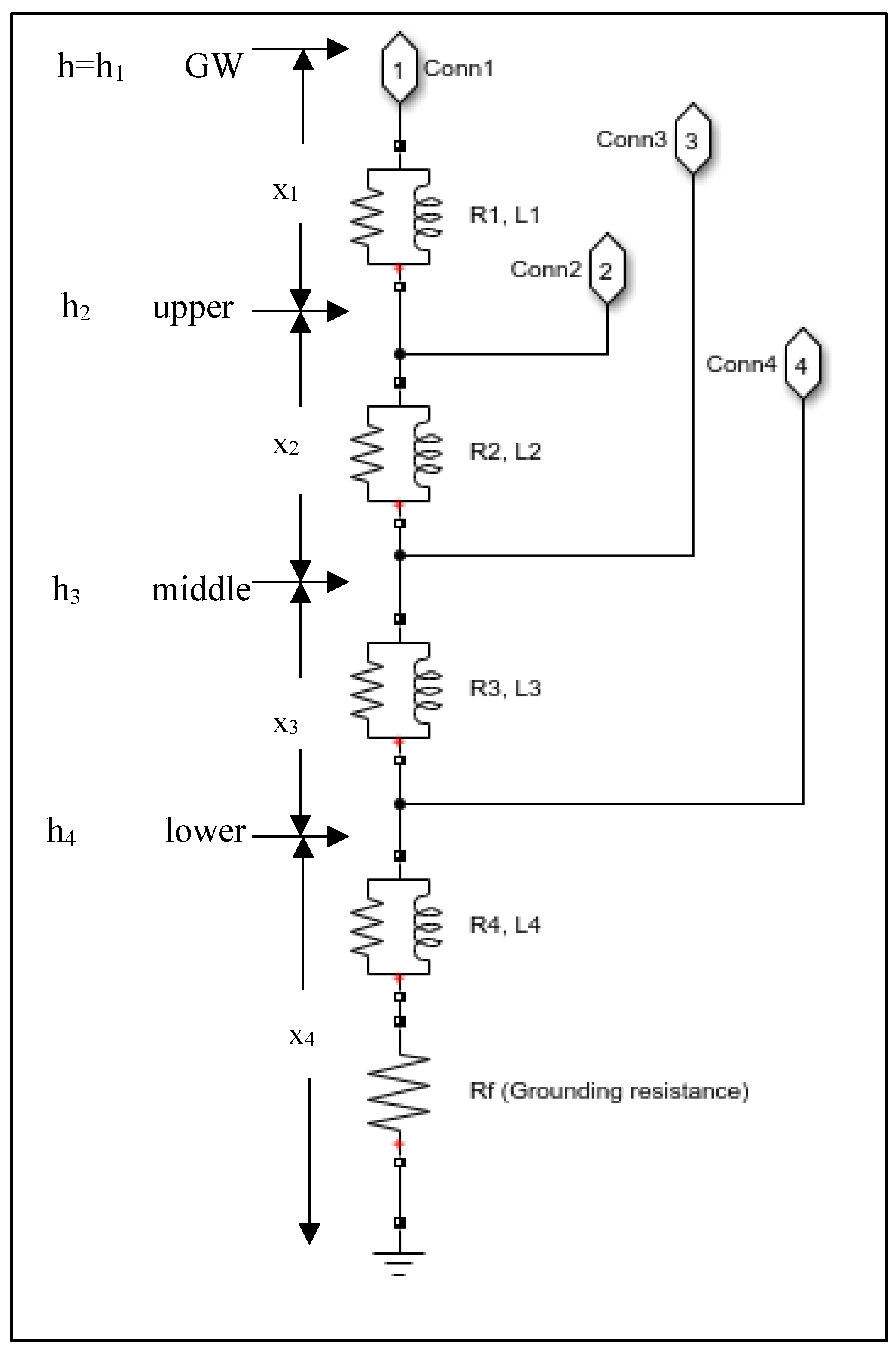
2.2.4. Lightning Fault Model

The lightning current is represented by a Norton circuit with a current source (Iy) of 40 kA in parallel with an impedance (Ry) in Figure 5. The impedance of the lightning channel is considered to be of about 400 ohms, although the CIGRE, IEC, and IEEE standards assume higher values [25,26]. The tower electrical parameters for an overhead line of 275 kV are presented in

Table 3. Tower model parameters for 275 kV system voltage [26].

Tower Height/Geometry (m)					Surge Impedance (Ω)		Footing Resistance (Ω)	Lightning Speed	Attenuation
$h_t$	h1	h2	h3	h4	Zt1	Zt4	Rf	$c_0$ m/μs	a1
31.76	2.70	5.55	5.55	17.96	220	150	5	300	0.89

, considering also a tower footing resistance in series with the entire structure. The parameters are established considering the model proposed by [26].

The multistory type tower model is used in this study where it is composed of four main parts representing the tower section between the cross arm, as illustrated in Figure 6. Each section consists of a lossless line in series with a parallel R-L circuit, included for attenuation of the traveling waves along the tower, a₁. The propagation velocity of a traveling wave along the tower, C₀ is assumed equal to 300 m/μs. Note that the overvoltage that can be obtained by means of simulation, when the simplest models are used, should be the same between terminals of all insulator strings since these models do not distinguish between line phases. In fact, some differences will be expected due to the different coupling between the shield wires and the phase conductors located at different heights above the ground. Meanwhile, this study will not vary the tower height as we maintained the use for 275 kV system voltage from Tenaga Nasional Berhad (TNB).

A transmission tower is represented by four distributed-parameter lines as defined in Table 3, where $Z_{t1}$ is surge impedance of tower top to the upper phase arm which is equivalent to the upper to middle and middle to lower. Meanwhile, $Z_{t4}$ is the surge impedance of tower to tower bottom. The value of R and L are defined using the following expression in (11) to (13) where the h_i were indicated in Figure 6.

$$R_i=\Delta R_i·h_i , L_i=2\tau R_i \left(i=1-4\right)$$

(11)

where $\tau =h_t/c_0$: travelling time along the tower.

$$\Delta R_1=\Delta R_2=\Delta R_3=\frac{2Z_{t1}·\ln \left(\frac{1}{{\alpha }_1}\right)}{h_t-h_4}$$

(12)

$$\Delta R_4=2Z_{t4}·\ln \left(\frac{1}{{\alpha }_1}\right)/h_t$$

(13)

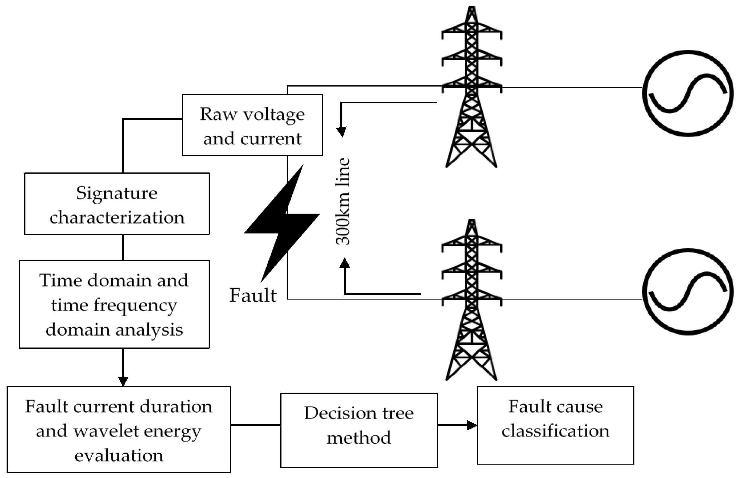
3. Proposed Methodology

This section provides the characterization of fault signal and its classification algorithm method.

3.1. Characterization of the Root Cause of Fault

Characterizing the fault is the process of determining the relevant features of root-cause of fault as well as finding indicators capable of measuring these features. Based on the results of the actual data acquisition, the characteristics of the fault are observed. The task of searching for indicators is one of the key steps in this research; that leads to the highest accuracy to be considered to describe and characterize the fault. This study has a clear achievement of fault detection; where most of the indicators of fault occurrences can be categorized as follows: the fault current duration increases from 10% to 90% of maximum value, fault current duration at 20% and fault current duration at 50% of maximum value. In addition, other evidences of fault can be observed, which shows the voltage dip percentage and energy wavelet of voltage waveform extracted, as shown in Figure 7, Figure 8, Figure 9 and Figure 10. The features are extracted from RMS current and voltage waveform where the equations involved in the waveform characteristics are explained in the following subsection.

3.1.1. Fault Current Duration

The RMS fault current duration characteristics rising from 10% to 90% are extracted as they provide a picture of the dynamic state of the fault during the initial transient stage. This gives an indication of the rate of change of current relative to the network or load prior to the fault occurrences. Equation (14) below described the equation of $T_{10/90}$. where represented current duration rise from 10% to 90% of maximum value.

$$T_{10/90}=T_{0.9Imax}-T_{0.1Imax}$$

(14)

The fault current duration at 20% of maximum waveform is extracted as it gives an indication of the dynamic state of fault at steady stage. The underlying mechanism by which fault current moves, differs for each of the major fault causes. Tree encroachment and crane encroachment fault current flows via the high impedance medium whilst fault current due to lightning is conducted via air particles. The resistivity of these medium differs significantly, as well as the duration of fault. The equation used to calculate fault current duration at 20% is:

$$T_{20}=\max (T_{0.2Imax})-\min \left(T_{0.2Imax}\right)$$

(15)

The fault current duration at 50% from the maximum waveform is extracted as it gives an indication of the dynamic state of fault at the final stage before fault extinction. The equation used to calculate fault current duration at 50% is:

$$T_{50}=\max (T_{0.5Imax})-\min \left(T_{0.5Imax}\right)$$

(16)

Figure 7 illustrates the current duration extracted from RMS waveform used in this study.

3.1.2. Voltage Dip

The RMS voltage dip of fault is evaluated based on two cycle window length which is equivalent to 200 samples. These features indicate a degree of unbalance during fault occurrences. Maximum voltage which is half cycle before the fault initiated is deducted with the minimum voltage value at the last point at which the 2nd cycle is calculated. The percentage of voltage dip value is then evaluated. Figure 8 illustrates an example of voltage dip with the minimum voltage indicated. The minimum voltage dip during the fault is calculated relatively with the maximum value as:

$$Vd={\left(Vmax-Vmin\right)}_{rms}\times 100$$

(17)

3.1.3. Time-Frequency Domain Analysis Using Discrete Wavelet Transform (DWT)

This subsection describes the time-frequency domain analysis of voltage signal using DWT. The DWT which is time-frequency analysis has been deployed as it was capable to extract features in time resolution and frequency resolution respectively [27,28,29,30]. The detail wavelet transform with mathematical algorithm is discussed in the subsequent section.

(a)

Discrete Wavelet Transform Algorithm

Wavelet transform is a powerful signal processing tool used in recognizing power disturbance pattern based on its features extraction [31]. It has the capability to analyze the signal in multi resolution either localized in time or space. Previously, Fourier Transform was used to analyze the stationary signal with limited capability for non-stationary analysis as the time information was lost [31]. Fourier Transform equation based on frequency domain can be defined as:

$$F\left(\omega \right)={{\displaystyle \int }}_{-\infty }^{+\infty }f\left(t\right)e^{-j\omega t}dt$$

(18)

From the equation, −∞ to +∞ indicated that time information will be lost. Therefore, the wavelet transform is an effective tool to analyze non stationary signal because of the mother wavelet function used as the basis function. Mother wavelet function $\mathsf{\psi } \left(\mathrm{t}\right)$ equation is defined as:

$$\mathsf{\psi } {\left(\mathrm{t}\right)}_{\left(a,b\right)}=\frac{1}{\sqrt{a}}\mathsf{\psi }\left[\frac{t-b}{a}\right]$$

(19)

where 1/a is frequency and $1\sqrt{a}$ is the normalizing constant of each scale parameter. Meanwhile, $b$ is parallel translation of time axis. The continuous wavelet transform (CWT) is defined as:

$$CW{T}_{\psi }x\left(a,b\right)=\frac{1}{\sqrt{\left|a\right|}}{{\displaystyle \int }}_{-\infty }^{+\infty }x\left(t\right){\psi }^{*}\left(\frac{t-b}{a}\right)dt$$

(20)

Terms $a$ and$b$ indicate the dilation and translation which determined the frequency length of wavelet and shifting position respectively. The $\psi$ is the mother wavelet, the $\ast$ indicates that the complex conjugate was used in the case of a complex wavelet. The extension of CWT, known as the discrete wavelet transform (DWT) is introduced to overcome the computational derived from CWT. The DWT is defined as:

$$DWT\left(m,n\right)={{\displaystyle \int }}_{-\infty }^{+\infty }x\left(t\right){\psi }_{m,n}^{*}\left(t\right)dt$$

(21)

where; ${\psi }_{m,n}\left(t\right)=a_0^{\raisebox{1ex}{$-m$}\!\left/ \!\raisebox{-1ex}{$2$}\right.}\left(\frac{(t-n{a}_0^m{b}_{0)}}{a_0^m}\right)$

These parameters are a = $a_0^m$, $b=n{b}_0{a}_0^m$

Where $m, n Z; m, n$represent the frequency localization and time localization respectively. The $x\left(t\right)$ denoted as signal in time domain. In this paper, db4 mother wavelet is used to detect the disturbance signal and obtain time detection information and detail frequency.

(b)

Decomposition

Discrete wavelet transform is a very useful technique to analyze the transient phenomenon. Multiresolution analysis (MRA) is one of the tools of DWT, which decomposes a non-stationary signal into low frequency signal known as approximation and high frequency signal called details. In this stage, the original disturbance waveforms are decomposed using DWT at the desired level j with “Daubechies” wavelet function of order n. The decomposition of PQ waveform into various frequency bands is achieved by applying high pass filter and low pass filter to the time domain signals. The flow of division filters is further explained in the next subsection. Figure 9 (D4)–(D1) illustrates four level decomposition coefficient of voltage dip fault utilised in this paper.

(c)

Sub-Band Filters

In DWT, the signal is analyzed at different frequency bands with different resolutions using the digital filtering techniques. This is significant to divide the signal into approximation and detail signals. The signal will comply into high pass and low pass filters. At the first stage, an original signal is slashed into two halves of bandwidth and shipped to both the filters. Next, the output of the low pass filter is further divided into half of the frequency bandwidth, and further shipped for the next stage. The step is iterated until at the agreed level, which are four levels in this case, and this is known as iterated filter bank. The accumulation of detailed information is measured by resolution of the signal, which is altered by filtering operations and the scale is rectified by the down sampling and up sampling operations.

The relation between low pass and high pass filters with the mother wavelet or known as scalar function $\psi \left(t\right)$ and the wavelet function $\varphi \left(t\right)$ can be defined as follows:

$$\varphi \left(t\right)={\displaystyle \sum }_{k}g\left[k\right]\varphi \left[2t-k\right]$$

(22)

$$\psi \left(t\right)={\displaystyle \sum }_{k}h\left[k\right]\varphi \left[2t-k\right]$$

(23)

The relation between the low pass filter and high pass filter is not independent to each other, but instead they are related by:

$$h\left[L-1-n\right]={\left(-1\right)}^{n}g\left[n\right]$$

(24)

where $g\left[n\right]$ is the low pass filter, $h\left[n\right]$ is the high pass filter,$L$ is the filter length (total number of points).

The impulse response $h\left[n\right]$ is involved while dispatching the signal across a half band low pass filter. The mathematical of convolution operation of the signal while filtering processes in discrete time is defined as follows:

$$A^0\left[n\right]\times h\left[n\right]={\displaystyle \sum }_{k=-\infty }^{\infty }{A}^0\left[n\right]·h\left[n-k\right]$$

(25)

Here $h\left[n\right]$ can be any filter’s impulse response.

$$y_n\left[k\right]={\displaystyle \sum }_{-\infty }^{\infty }x\left[n\right]·h\left[2n-k\right]$$

(26)

Based on Equations (27) and (28), the high and low frequency are derived as following definition:

$$y_{high}\left[k\right]={\displaystyle \sum }_n{A}^0\left[n\right]·g\left[2k-n\right]$$

(27)

$$y_{low}\left[k\right]={\displaystyle \sum }_n{A}^0\left[n\right]·h\left[2k-n\right]$$

(28)

where $y_{high}\left[k\right]$ and $y_{low}\left[k\right]$ are the yields of the high pass and low pass filters after subsampling by 2. Here $y_{high}\left[k\right]$ is denoted as the detailed component and $y_{low}\left[k\right]$ denoted as the approximate component. $A^0$ denoted as input signal. The algorithm of sub-band filter for high-pass filter and low pass filter of wavelet decomposition in levels of approximated and detailed coefficients were denoted in [32]. After the decomposition process, the wavelet signal will be reconstructed and all reconstructed energy level will be combined to obtain the fix value. At this stage, the higher noises, where the fault signal deviates more from the normal one, will produce more energy. However, an absolute energy value is evaluated above the set up threshold. In this case, the initiated threshold value is 10% of the maximum magnitude. Figure 10 illustrates the reconstructed coefficient energy that is extracted from voltage dip fault signal and used in this study.

3.2. Decision Tree Algorithm

The decision tree classification has advantages in terms of flexibility, nonparametric nature and capable to handle non-linear relations between features and classes. An input sample can be classified into its possible classes through tree structures of decision tree formation [14,33]. The tree structures formation defined in decision rules model within based on if/else instruction. The decision tree is one of the well-known classification tools since it gives prudent accuracy and low cost computation [11]. In this paper, the decision tree application i.e., a type of supervised learning, is simulated in MATLAB using ‘fitctree’ command. The targeting output will supervise the training sets using recursive binary partitioning method. Succeeding questions with yes or no results are inquired for separating the sample space. The nodes are the spots where the test is performed on the elements. The test results then are represented to another node that could be seen as branches. There are three kinds of node presenting in decision tree namely the root node, the leaf node, and the internal node, as illustrated in Figure 11. The outcome of the test is determined by the purity of each node. The node will stop once it achieves an optimal post level of class purity. The optimal level is defined when the node is having the only output types in the node. An element value will be tested against the decision tree whenever to classify the new samples. Class prediction for the tested samples is maintained by the attribution path from the root node to a leaf node. The basic process of getting a decision tree is to repetitively find the attribute to be tested on a node and then subsidiary to another node. This whole attribution process to identify test and branch is known as splitting.

The splitting process has a role to minimize the impurity in the dataset which corresponding to class at the later stage. The process requires information gain calculation which must be accomplished into two stages which are entropy and entropy splitting index. Based on the Figure 11b $t_P$ is parent node, $t_L$ is left child node, and $t_R$—right child node. The entropy index also known as impurity and the measure of impurity/entropy i(t) at node t is denoted as;

$$i\left(t\right)=-{{\displaystyle \sum }}_{j=1}^{k}p\left(w_j|t\right)\log p\left(w_j|t\right)$$

(29)

where $p\left(w_j|t\right)$ is the proportion of the pattern $x_j$ allocated to class $w_j$ at node $t$. Each non-terminal node is divided into node $t_L$ and $t_R$ as shown where $x_j^R$ represented the best splitting values of variable $x_j$. Corresponding proportions of entities new node are $P_L$ and $P_R$. The best division (entropy splitting index) is that which maximized the difference is given by Equation (30).

$$\Delta i\left(t\right)=i\left(t_P\right)-P_{R}i\left(t_L\right)-P_{L}i\left(t_R\right)$$

(30)

Furthermore, to find the best split predictor at each node, this study implemented selection predictor algorithm namely all splits, curvature, and interaction-curvature. All splits or standard classification decision trees will select the split predictor that maximizes the split-criterion gain over all possible splits of all predictors. Curvature selects the split predictor that minimizes the p-value of chi-square tests of independence between each predictor and the response. Training speed is similar to standard classification decision tree. Finally, interaction-curvature will choose the split predictor that minimizes the p-value of chi-square tests of independence between each predictor and the response, and that minimizes the p-value of a chi-square test of independence between each pair of predictors and response. Training speed can be slower than standard classification decision tree [34,35,36].

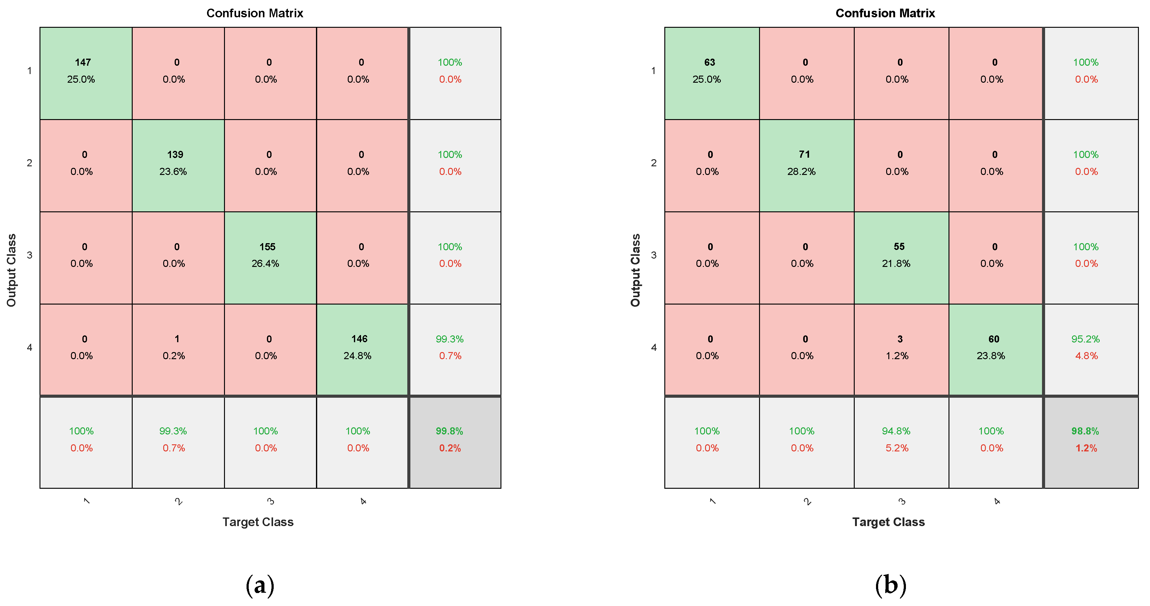
3.3. Confusion Matrix Algorithm

The confusion matrix contains the information about the predicted and actual classification. The confusion matrix is usually in the form of a table and is utilized to evaluate the performance of the classifier on a set of testing data where the true value is established. Figure 12 illustrates the basic terms in the confusion matrix formed in the table. The terms are usually in a form of whole number:

• True Positive (TP) is the cases that we predicted yes and they do have the cases.
• True Negative (TN) is the cases that we predicted no and they do not have the cases.
• False Positive (FP) is the cases that we predicted yes but they do not have the cases.
• False Negative (FN) is the cases that we predicted not but they do have the cases.

Based on the confusion matrix basic terms, a list of rates that execute the classifier performance is computed.

Table 4. List of rates definition computed from the confusion matrix.

Symbol	Matrix	Definition
ACC	Accuracy	$\frac{TP+TN}{TP+TN+FP+FN}$
SNS	Sensitivity	$\frac{TP}{TP+FN}$
SPC	Specificity	$\frac{TN}{TN+FP}$
PRC	Precision	$\frac{TP}{TP+FP}$
F1	F1 Score	$2\frac{PRC·SNS}{PRC+SNS}$

indicates the list of rates with their definition used in this paper. There are five rates that have been used which are accuracy, sensitivity, specificity, precision, and F₁ score.

4. Result and Discussion

4.1. Fault Model Validation Result

The fault model proposed in the study was validated by comparing the simulation result with field data acquired from the fault recorder. Current waveform generated from the simulation was validated by evaluating its root mean square error (RMSE) for each cases. The equation of the RMS is defined as:

$$RMSE=\sqrt{{\overline{\left(x-x_i\right)}}^2}$$

(31)

where $x$ is the actual waveform while $x_i$ is the generated waveform. Detail validation result is described in the following subsection.

Figure 13a illustrates the generated simulation and actual waveform due to lightning strike. The generated waveform of 180-degree inception angle and 330 MVAR load were chosen for comparison with the actual fault occurs within 20 km from the substation. The RMSE value of the generated waveform current is 0.0342. Figure 13b illustrates the generated simulation and actual waveform due to insulator degrading. The RMSE generated waveform of 180-degree inception angle and 330 MVAR load was evaluated with actual fault occurs within 60 km from the substation, which gives the value of 0.0498. Furthermore, Figure 13c illustrates the generated simulation and actual waveform due to the tree encroachment. The actual waveform was taken on 30th December 2019 during the fault occurrence. The generated waveform chosen at 30-degree inception angle and 330 MVAR load was compared with the actual fault that occured within 10 km from the substation. The RMSE value of generated waveform current and is 0.0696. Meanwhile, Figure 13d illustrates the generated simulation and actual waveform due to crane encroachment. The generated waveform with fault triggered at 30-degree inception angle and 330 MVAR load is evaluated based on actual fault occurrences within 30 km from the substation. The RMSE value of generated waveform current is 0.0498. Therefore, the RMSE value of all simulated fault causes are less than 0.1 which is considered small and indicated the correctness of the models.

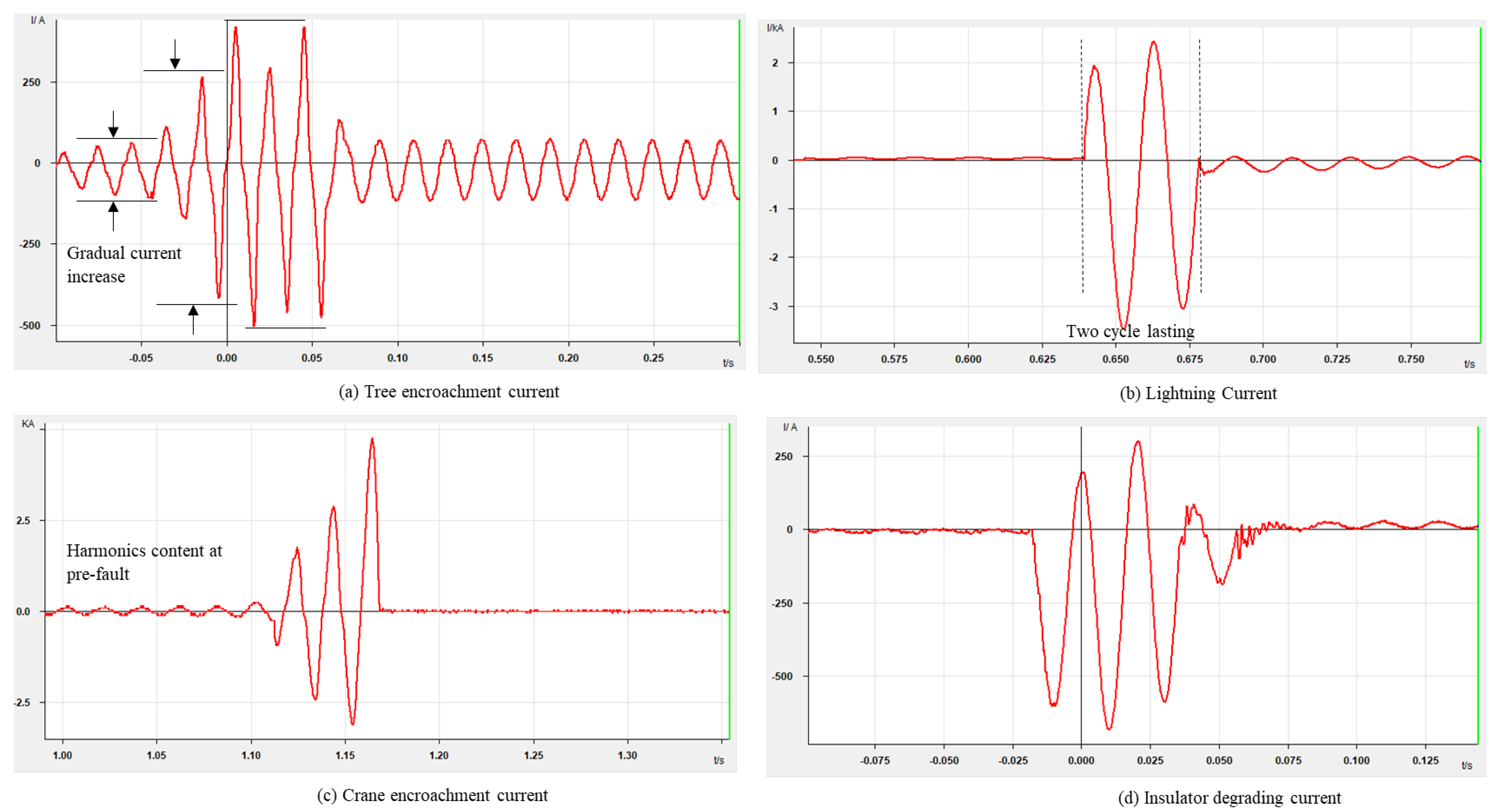
4.2. Fault Signature Characterization

Initially, the fault occurred in transmission line system is simulated based on signature obtained in raw neutral current and voltage signal. Single line to ground fault have been chosen for this study due to the fact that it is the most prominent fault types among the line to line fault, the double line to ground fault, and the three phase fault. Moreover, four types of faults namely lightning, insulator degrading, tree encroachment, and crane encroachment are chosen according to their prominent tripping occurred in Malaysia within the year 2016 to 2020. The signatures of faults based on neutral current and voltage waveform, which have different patterns, can be observed in Figure 14 and Figure 15a–d.

Based on the Figure 14a, tree encroachment shows a gradual current increase that lasted for six cycles. Whilst lightning fault shows current increase which lasting for two cycles and with high magnitude of about 2 kA Figure 14b. In some cases, the lightning fault can last for three to three and half cycle. As for the crane encroachment, fault current indicates a gradual increase lasting for three cycles which contains harmonic content at the pre-fault as shown in Figure 14c. Finally, for insulator degrading (Figure 14d), the fault current increases within three cycles, which is the same pattern as per lightning fault but with a lower magnitude. However, fault current for lightning is usually higher than insulator degrading due to its high current which can be up to thousands of kiloamps, which is dependent on the load carried in the lines. The higher the loads, the greater the fault current magnitude.

In addition, the criteria of faults were observed on the voltage signature. Based on the Figure 15a,c, sinusoidal voltage pattern for tree encroachment and crane encroachment has no difference from the normal condition until the circuit breaker is closed. Meanwhile, Figure 15b shows a voltage dip of more than 20% was produced in the system for lightning with a slight dip in the case of insulator degrading as in Figure 15d Based on the observation, raw voltage and current fault did give several signatures but insufficient to be analyzed due to similar characteristics obtained in several cases. Therefore, further analyses such as converting the raw current and voltage into RMS and DWT have been considered and proposed in this paper.

4.3. Decision Tree Method Sample Selection

This subsection explores the performance of the decision tree classification method in detecting the four types of faults during operation. All extracted features are implemented in MATLAB, where a set of 840 samples contained four types of fault are mixed randomly and trained into the classification system. Several parameters in the decision tree namely the maximum number of splits and predictor selection are varied to find the best classifier to be used in the study based on its percentage accuracy. Furthermore, the confusion matrix algorithm is adopted in the decision tree to present the performance of classification accuracy of the fault causes.

Table 5. Input and target output sampled used for decision tree.

Sample	Input					Categorical Variable/Output
	Var 1	Var 2	Var 3	Var 4	Var 5
1	0.0142	0.0720	0.0596	7.7798	0.1695	2
2	0.0136	0.0826	0.0768	39.3691	0.9252	1
3	0.0150	0.0708	0.0580	9.1606	0.2659	2
4	0.0138	0.0712	0.0584	6.7943	0.1474	2
5	0.1208	0.1462	0.0368	2.2889	0.0054	3
6	0.1072	0.1228	0.0799	0.5959	0.0014	3
7	0.0142	0.0724	0.0632	10.8221	0.1757	2
8	0.0142	0.0816	0.0680	28.7403	0.7757	1
8	0.0688	0.0878	0.0764	0.3635	0.0003	4
10	0.0278	0.0224	0.0000	0.7551	0.0022	4
11	0.0184	0.0698	0.0572	13.6512	0.5133	2
12	0.0184	0.0814	0.0660	40.7826	1.0624	1
13	0.1200	0.1588	0.0487	0.6651	0.0010	3
14	0.1192	0.2138	0.0387	3.5494	0.0069	3
15	0.1158	0.2780	0.0392	0.8545	0.0024	3

shows a set of 10 samples containing five variables as the input data and those four types of fault were assigned as 1, 2, 3, and 4, respectively.

Table 6. Description for input and target output label.

	Label	Description	Unit
Input	Var 1	Fault duration from 10% to 90% increase (T10/90)	s
	Var2	Fault duration from at 20% increase (T20)	s
	Var 3	Fault duration from at 20% increase (T50)	s
	Var 4	Voltage drop (Vd)	%
	Var 5	Wavelet energy (Ener)	-
Categorical variable / Output	1	Lightning	-
	2	Insulator degrading	-
	3	Tree encroachment	-
	4	Crane encroachment	-

defines the actual output variables which later to be set as an array in the system to ease the computation process.

Figure 16 shows the decision tree diagram with the average number of splits of five which is not cross validated at the early stage. The root node of the features is T1090 whereby if the duration is greater or equal to 0.0857 s, then the fault is defined as tree encroachment. Otherwise, if it is less than 0.0857 s, it will create another internal node. If the voltage dip is equal to or greater than 19.52%, the fault cause is termed as lightning, or else, it creates the other internal node. Next, if the wavelet energy is less than 0.113, the leaf node is concluded as the crane encroachment. Otherwise, the decision tree will look into T50 and T20. Based on these two features, the faults can be categorized as a crane or insulator degrading. If the T50 is less than 0.0599 s, and T20 is greater than or equal to 0.0716, the leaf node is defined as insulator degrading. Otherwise, if T50 is greater than or equal to 0.0599 s and T20 less than 0.0716, the fault causes are concluded as the crane encroachment.

In addition, the decision tree is cross-validated using 10 fold and iterated 10 times with a different maximum number of splits set up. In this study, the maximum number of splits are evaluated between 1 to 10 with the accuracy of each splits is then evaluated.

Table 7. Percentage accuracy for different maximum number of split set up.

Iteration (ith)	Percentage Accuracy (%)	Maximum Number of Split
1	52.0408	1
2	76.5306	2
3	99.8299	3
4	99.8299	4
5	99.4898	5
6	99.4898	6
7	99.3197	7
8	99.8299	8
9	99.8299	9
10	99.6599	10

shows the least percentage accurate obtained when the number of splits is set at 1 which is 52.048% while the highest percentage accuracy is obtained when the number of splits is set at 3, 4, 8, and 9 which is translated in 99.829%. This defines that the minimum of split with the highest accuracy, which is 3, was indicated as an optimum number of split chosen. Therefore, the decision tree algorithm with a number of splits of 3 is considered and implemented in the next process.

4.4. Decision Tree Classification Performance of Fault Causes Based on Different Predictor Selection

A test set of 30% and 20% sample sizes are created to be tested in the decision tree algorithm. The test set ratio are randomly selected using MATLAB command to become an input of creating the decision tree while the targeted output is validated based on classification criteria. The training set of 70% and test set of 30% data samples are described in

Table 8. Accuracy of the created decision tree w.r.t. all splits predictor selection on test set data for 70% training and 30% testing.

Train/Test	Lightning	Insulator	Tree	Crane
Lightning	100% (63/63)	-	-	-
Insulator	-	100% (71/71)	-	-
Tree	-	-	100% (55/55)	-
Crane	-	-	-	100% (63/63)

,

Table 9. Accuracy of the created decision tree w.r.t. curvature predictor selection on test set data for 70% training and 30% testing.

Train/Test	Lightning	Insulator	Tree	Crane
Lightning	100% (63/63)	-	-	-
Insulator	-	100% (71/71)	-	-
Tree	-	-	100% (55/55)	-
Crane	-	-	3	85.71% (60/63)

and

Table 10. Accuracy of the created decision tree w.r.t. interaction-curvature predictor selection on test set data for 70% training and 30% testing.

Train/Test	Lightning	Insulator	Tree	Crane
Lightning	98.4% (62/63)	1	-	-
Insulator	-	100% (71/71)	-	-
Tree	-	-	100% (55/55)	-
Crane	-	-	-	100% (63/63)

. Based on Table 8, the classification accuracy of fault with respect to all splits predictor selection is evaluated where it gives 100% prediction accuracy. Meanwhile, Table 9 provides the classification accuracy of the decision tree for a fault that occurred when the predictor selection is set as curvature. It can be observed that three samples of crane encroachment are misclassified into tree encroachment region, resulting in about 85.71% accuracy. Furthermore, the classification accuracy based on the interaction-curvature of predictor selection adopted in the study is evaluated in Table 10. From the table, it can be observed that one sample of lightning is misclassified into insulator degrading region which makes the classification error increase by 1.6%. In summary, based on Table 8, Table 9 and Table 10, the decision tree classification has an average prediction accuracy of 97.4% although there are misclassifications recorded for each case.

On another case, the training set of 80% and test set of 20% data samples are described in

Table 11. Accuracy of the created decision tree w.r.t. all splits predictor selection on test set data for 80% training and 20% testing.

Train/Test	Lightning	Insulator	Tree	Crane
Lightning	100% (38/38)	-	-	-
Insulator	-	100% (44/44)	-	-
Tree	-	-	100% (48/48)	-
Crane	-	-	1	97.4% (37/38)

,

Table 12. Accuracy of the created decision tree w.r.t. curvature predictor selection on test set data for 80% training and 20% testing.

Train/Test	Lightning	Insulator	Tree	Crane
Lightning	100% (42/42)	-	-	-
Insulator	-	100% (50/50)	-	-
Tree	-	-	100% (35/35)	-
Crane	-	-	-	100% (41/41)

and

Table 13. Accuracy of the created decision tree w.r.t. interaction-curvature predictor selection on test set data for 80% training and 20% testing.

Train/Test	Lightning	Insulator	Tree	Crane
Lightning	100% (55/55)	-	-	-
Insulator	-	100% (37/37)	-	-
Tree	-	-	100% (32/32)	-
Crane	-	-	3	93.2% (41/44)

. When all splits predictor selection is adopted to the created decision tree, one sample from crane encroachment region was misclassified as a tree encroachment region, resulting in 97.4% prediction accuracy. Apart from that, the rest of the regions resulted in 100% accuracy without any misclassification samples. Whilst, the classification accuracy of the decision tree for fault causes with respect to the curvature predictor selection is provided in Table 12. It can be observed that all fault causes are correctly classified and thus, gives 100% prediction accuracy. The classification accuracy of the decision tree for fault classification with respect to interaction-curvature is provided in Table 13. Three samples from crane encroachment regions are misclassified into tree encroachment and thus resulted in the lowest prediction accuracy which is 93.2%. Overall, it can be concluded that although there are misclassification occurred, each decision tree has an average prediction accuracy of 96.87% which is considered appropriate and high accuracy, as depicted in Table 11, Table 12 and Table 13.

4.5. Computational Time

The proposed method also compares the computation time of each predictor selection.

Table 14. Computation time of the decision tree method for different predictor selection.

Sample Ratio	Computation Time (s)
	All Splits	Curvature	Interaction-Curvature
70/30	11.622430	12.270969	11.688976
80/20	12.392414	12.783483	11.775463

describes the computation time of each predictor selection. Overall, the computation time of each predictor selection with both sample ratios is nearly the same. However, when zooming further, all splits predictor with sample ratio of 70/30 computed the processing code at the fastest rate with 11.622430 s while curvature predictor at sample ratio of 80/20 resulted at the slowest rate.

4.6. Confusion Matrix Performance for Decision Tree on Different Predictor Selection

The confusion matrix presents the performance of the decision tree based on different predictor selection and different testing samples. Figure 17 illustrates the forms of confusion matrix for the decision tree method. In this study, one versus one (OVO) error correcting output codes (ECOC) have been trained, and ensemble Bag parameters as binary learner are implemented to outperform multiclass output. Accuracy, sensitivity, specificity, precision, and F₁ scores are extracted from the confusion matrix as shown in

Table 15. Confusion matrix performance.

Fault Causes	Sample Size	Predictor Selection	ACC	SNS	SPC	PRC	F1
			(%)
Lightning	30% test	All splits	100	100	100	100	100
		Curvature	100	100	100	100	100
		Interaction- curvature	98.90	100	94.50	94.80	97.30
	20% test	All splits	100	100	100	100	100
		Curvature	100	100	100	100	100
		Interaction- curvature	100	100	100	100	100
Insulator degrading	30% test	All splits	100	100	100	100	100
		Curvature	100	100	100	100	100
		Interaction- curvature	99.60	100	99.40	98.60	99.30
	20% test	All splits	100	100	100	100	100
		Curvature	100	100	100	100	100
		Interaction- curvature	100	100	100	100	100
Tree encroachment	30% test	All splits	100	100	100	100	100
		Curvature	98.80	100	98.50	94.80	97.30
		Interaction- curvature	100	100	100	100	100
	20% test	All splits	99.40	100	99.20	98.00	99.00
		Curvature	100	100	100	100	100
		Interaction- curvature	98.20	100	97.80	91.40	95.50
Crane encroachment	30% test	All splits	100	100	100	100	100
		Curvature	98.80	95.20	100	100	97.50
		Interaction- curvature	100	100	100	100	100
	20% test	All splits	99.40	97.40	100	100	98.70
		Curvature	100	100	100	100	100
		Interaction- curvature	98.20	93.20	100	100	96.50

.

The fault due to lightning when tested with 30% and 20% data set shows the best performance (100%) for all predictor selection except for interaction-curvature where the accuracy, specificity, precision, and F₁ score are 98.8%, 94.5%, 94.8%, and 97.3%, respectively. In addition, the same pattern was obtained for fault due to insulator degrading where interaction-curvature gives the worst performance as compared with the other predictor selection. The accuracy of the confusion matrix is 99.6%, with specificity is 99.4%, precision is 98.6% and F₁ score is 99.3%. As for the tree encroachment, more misclassified data were obtained as compared to the lightning and insulator degradation where the confusion matrix performance is also lower. Based on the table, curvature predictor selection shows the worst performance when the tested sample is 30%, while all splits and interaction-curvature shows low performance when the tested sample is 20%. However, among all of them, interaction-curvature gives the worst predictor selection performance with only 98.2% accuracy, 97.8% specificity, 91.4% precision, and 95.5% F1 score. Finally, fault cause due to crane encroachment shows the worst performance when using curvature predictor selection for 30% tested sample and interaction-curvature predictor selection gives worst performance for 20% tested sample.

Overall, the predictor selection of interaction-curvature gives the worst performance for this classification application and all splits give the best performance for most of the faults classified. Therefore, it can be concluded that several samples are misclassified due to the confusion features where the system sees the similar features for different faults. On another note, the best predictor selection for this classification is all splits.

5. Conclusions

This paper outlined the fault signatures that occurred in transmission line networks by characterizing and classifying using the decision tree classification method. The RMS fault current duration and voltage dip percentage, as well as DWT, were evaluated for several cycles during the fault condition. One could infer that the proposed fault classification technique is simple and can accomplish extremely high precision where most of the classifier recorded performance greater than 93%, with computation time within 12.089 s on average. Classification using a decision tree is without much of a stretch to handle both numerical and categorical variables. The method can lift the decision list, incorporate with the search steps, apply the decision tree rules on the fault detection and also improve the accuracy of fault tree classification. Among other advantages of the decision tree method is its endurance to outliers, where the splitting algorithm will usually separate the outliers into individual node or nodes. An important practical property of a decision tree is that the structure of its classification trees is invariant with respect to monotonic transformations of independent variables. One can replace any variable with its logarithm or square root value, without the need to change the structure of the tree. Supervised fault classification with decision tree analysis is a successful method and effectively implemented for creating a ruled-based classification when expert knowledge is inadequate.

References

1. Carlsson, F.; Kataria, M.; Lampi, E.; Martinsson, P. Past and present outage costs—A follow-up study of households’ willingness to pay to avoid power outages. Resour. Energy Econ. 2021, 64, 101216. [Google Scholar] [CrossRef]
2. Saravanan, N.; Ramachandran, K.I. Incipient gear box fault diagnosis using discrete wavelet transform (DWT) for feature extraction and classification using artificial neural network (ANN). Expert Syst. Appl. 2010, 37, 4168–4181. [Google Scholar] [CrossRef]
3. Rodrigues, M.A.P.; Souza, J.C.S.; Schilling, M.T.; Filho, M.B.D.C. Fault diagnosis in electrical power systems using artificial neural networks. Int. Conf. Electr. Power Eng. Power Tech. Bp. 1999, 2, 130. [Google Scholar]
4. Asman, S.H.; Ab Aziz, N.F.; Abd Kadir, M.Z.A.; Amirulddin, U.A.U. Fault signature analysis based on digital fault recorder in malaysia overhead line system. In Proceedings of the 2020 IEEE International Conference on Power and Energy (PECon), Penang, Malaysia, 7–8 December 2020; pp. 188–193. [Google Scholar]
5. Kadir, M.Z.A.A.; Cooper, M.A.; Gomes, C. An overview of the global statistics on lightning fatalities. In Proceedings of the 30th InternationalInternational Conference on Lightning Protection-ICLP 2010, Cagliari, Italy, 13–17 September 2010; Volume 2010, pp. 1–4. [Google Scholar]
6. Asman, S.H.; Ab Aziz, N.F.; Abd Kadir, M.Z.A.; Amirulddin, U.A.U. Fault signature analysis for medium voltage overhead line based on new characteristic indices. In Proceedings of the 2020 IEEE International Conference on Power and Energy (PECon), Penang, Malaysia, 7–8 December 2020; pp. 198–203. [Google Scholar]
7. Emperuman, M.; Chandrasekaran, S. Hybrid Continuous Density Hmm-Based Ensemble Neural Networks for Sensor Fault Detection and Sensor Network. Sensors 2020, 20, 745. [Google Scholar] [CrossRef] [PubMed] [Green Version]
8. Guo, S.; Yang, T.; Gao, W.; Zhang, C. A Novel Fault Diagnosis Method for Rotating Machinary Based on a Convoluttional Neural Network. Sensors 2018, 18, 1429. [Google Scholar] [CrossRef] [PubMed] [Green Version]
9. Dhimish, M.; Holmes, V.; Mehrdadi, B.; Dales, M. Comparing Mamdani Sugeno fuzzy logic and RBF ANN network for PV fault detection. Renew. Energy 2018, 117, 257–274. [Google Scholar] [CrossRef] [Green Version]
10. Mustafa, M.; EI-Khattam, W.; Galal, Y. A novel fuzzy cause-and-effect-networks based methodology for a distribution system’ s fault diagnosis. In Proceedings of the 2013 3rd International Conference on Electric Power and Energy Conversion Systems, Istanbul, Turkey, 2–4 October 2013; pp. 1–6. [Google Scholar]
11. Han, H.L.; Ma, H.Y.; Yang, Y. Study on the Test Data Fault Mining Technology Based on Decision Tree. Procedia Comput. Sci. 2019, 154, 232–237. [Google Scholar] [CrossRef]
12. Saravanan, N.; Ramachandran, K.I. Fault diagnosis of spur bevel gear box using discrete wavelet features and Decision Tree classification. Expert Syst. Appl. 2009, 36, 9564–9573. [Google Scholar] [CrossRef]
13. Upendar, J.; Gupta, C.P.; Singh, G.K. Statistical decision-tree based fault classification scheme for protection of power transmission lines. Int. J. Electr. Power Energy Syst. 2012, 36, 1–12. [Google Scholar] [CrossRef]
14. Benkercha, R.; Moulahoum, S. Fault detection and diagnosis based on C4.5 decision tree algorithm for grid connected PV system. Sol. Energy 2018, 173, 610–634. [Google Scholar] [CrossRef]
15. Carpenter, M.; Hoad, R.R.; Bruton, T.D.; Das, R.; Kunsman, S.A.; Peterson, J.M. Staged-fault testing for high impedance fault data collection. In Proceedings of the 58th Annual Conference for Protective Relay Engineers, College Station, TX, USA, 5–7 April 2005; pp. 9–17. [Google Scholar]
16. AsghariGovar, S.; Pourghasem, P.; Seyedi, H. High impedance fault protection scheme for smart grids based on WPT and ELM considering evolving and cross-country faults. Int. J. Electr. Power Energy Syst. 2019, 107, 412–421. [Google Scholar] [CrossRef]
17. Kavi, M.; Mishra, Y.; Vilathgamuwa, M.D. High-impedance fault detection and classification in power system distribution networks using morphological fault detector algorithm. IET Gener. Transm. Distrib. 2018, 12, 3699–3710. [Google Scholar] [CrossRef]
18. Gautam, S.; Brahma, S.M. Detection of high impedance fault in power distribution systems using mathematical morphology. IEEE Trans. Power Syst. 2013, 28, 1226–1234. [Google Scholar] [CrossRef]
19. Soheili, A.; Sadeh, J.; Bakhshi, R. Modified FFT based high impedance fault detection technique considering distribution non-linear loads: Simulation and experimental data analysis. Int. J. Electr. Power Energy Syst. 2018, 94, 124–140. [Google Scholar] [CrossRef]
20. Wester, C.G. High impedance fault detection on distribution systems. In Proceedings of the 1998 Rural Electric Power Conference Presented at 42nd Annual Conference, St. Louis, MO, USA, 26–28 April 1999. [Google Scholar]
21. Silva, S.; Costa, P.; Gouvea, M.; Lacerda, A.; Alves, F.; Leite, D. High impedance fault detection in power distribution systems using wavelet transform and evolving neural network. Electr. Power Syst. Res. 2018, 154, 474–483. [Google Scholar] [CrossRef]
22. Silva, P.R.N.; Carvalho, A.P.A.; Vieira, P.; Costa, C.T. Characterization of failures in insulators to maintenance in transmission lines. In Proceedings of the 2017 IEEE International Conference on Smart Energy Grid Engineering, Oshawa, ON, Canada, 14–17 August 2017; pp. 7–13. [Google Scholar]
23. Waluyo; Pakpahan, P.M. Suwarno Study on the electrical equivalent circuit models of polluted outdoor insulators. IEEE 2006, 5–8. [Google Scholar]
24. Redfern, M.A.; Bo, Z.Q.; Montjean, D. Detection of broken conductors using the positional protection technique. Proc. IEEE Power Eng. Soc. Transm. Distrib. Conf. 2001, 2, 1163–1168. [Google Scholar]
25. Mariut, L.; Helerea, E. Electromagnetic Analysis—Application to Lightning Surge Phenomena on Power Lines. In Proceedings of the 2014 International Symposium on Fundamentals of Electrical Engineering, Bucharest, Romania, 28–29 November 2014; pp. 14–19. [Google Scholar]
26. CIGRE, W. Guideline for Numerical Electromagnetic Analysis Method and Its Application to Surge Phenomena. 2013. Available online: https://e-cigre.org/publication/543-guideline-for-numerical-electromagnetic-analysis-method-and-its-application-to-surge-phenomena (accessed on 20 April 2021).
27. Ijaz, M.; Shafiullah, M.; Abido, M.A. Classification of power quality disturbances using Wavelet Transform and Optimized ANN. In Proceedings of the 2015 18th International Conference on Intelligent System Application to Power Systems (ISAP), Porto, Portugal, 11–16 September 2015. [Google Scholar]
28. Gautam, N.; Ali, S.; Kapoor, G. Detection of fault in series capacitor compensated double circuit transmission line using wavelet transform. In Proceedings of the 2018 International Conference on Computing, Power and Communication Technologies (GUCON) Greater, Noida, India, 28–29 September 2019; pp. 760–764. [Google Scholar]
29. Kaitwanidvilai, S.; Pothisarn, C.; Jettanasen, C.; Chiradeja, P.; Ngaopitakkul, A. Discrete wavelet transform and back-propagation neural networks algorithm for fault classification in underground cable. In Proceedings of the IMECS 2011 International MultiConference of Engineers and Computer Scientists 2011, Hong Kong, China, 16–18 March 2011; Volume 2, pp. 996–1000. [Google Scholar]
30. Asman, S.H.; Aziz, N.F.A.; Kadir, M.Z.A.A.; Amirulddin, U.A.U.; Izadi, M. Determination of Different Fault Features in Power Distribution System Based on Wavelet Transform. Int. J. Recent Technol. Eng. 2019, 8, 6256–6261. [Google Scholar]
31. Chiradeja, P.; Pothisarn, C. Identification of the fault location for three-terminal transmission lines using discrete wavelet transforms. In Proceedings of the 2009 Transmission & Distribution Conference & Exposition: Asia and Pacific, Seoul, Korea, 26–30 October 2009; pp. 3–6. [Google Scholar]
32. Habsah Asman, S.; Farid Abidin, A. Comparative Study of Extension Mode Method in Reducing Border Distortion Effect for Transient Voltage Disturbance. Indones. J. Electr. Eng. Comput. Sci. 2017, 6, 628. [Google Scholar] [CrossRef]
33. Vanfretti, L.; Arava, V.S.N. Decision tree-based classification of multiple operating conditions for power system voltage stability assessment. Electr. Power Energy Syst. 2020, 123, 106251. [Google Scholar] [CrossRef]
34. Breiman, L.; Friedman, J.; Stone, C.J.; Olshen, R.A. Classification and Regression Trees; CRC Press: Boca Raton, FL, USA, 1984; ISBN 0412048418. [Google Scholar]
35. Loh, W.-Y. Regression tress with unbiased variable selection and interaction detection. Stat. Sin. 2002, 361–386. [Google Scholar]
36. Loh, W.-Y.; Shih, Y.-S. Split selection methods for classification trees. Stat. Sin. 1997, 815–840. [Google Scholar]
Figure 1. Transmission line fault simulation process.
Applsci 11 04031 g001
Figure 2. HIF model based on Emanuel arc model.
Applsci 11 04031 g002
Figure 3. Harmonics current injection.
Applsci 11 04031 g003
Figure 4. Fault impedance model of insulator failure.
Applsci 11 04031 g004
Figure 5. Norton circuit.
Applsci 11 04031 g005
Figure 6. Multistory tower model in MATLAB [26].
Applsci 11 04031 g006
Figure 7. Fault current criteria.
Applsci 11 04031 g007
Figure 8. Voltage dip criteria for fault causes.
Applsci 11 04031 g008
Figure 9. DWT process with four decomposition coefficient.
Applsci 11 04031 g009
Figure 10. Energy wavelet for combined reconstructed coefficient (a) and absolute value (b).
Applsci 11 04031 g010
Figure 11. Decision tree attributes (a) and division process (b).
Applsci 11 04031 g011
Figure 12. Confusion matrix table.
Applsci 11 04031 g012
Figure 13. Validation result for generated current waveform due to lightning (a), insulator degrading (b), tree encroachment (c), and crane encroachment (d).
Applsci 11 04031 g013
Figure 14. Fault signature of neutral current sinusoidal waveform.
Applsci 11 04031 g014
Figure 15. Fault signature for voltage phase sinusoidal waveform.
Applsci 11 04031 g015
Figure 16. Decision tree diagram of fault causes without cross-validated.
Applsci 11 04031 g016
Figure 17. Confusion matrix for training (a) and testing (b) performance of decision tree.
Applsci 11 04031 g017