Abstract
The use of unmanned aerial robots has increased exponentially in recent years, and the relevance of industrial applications in environments with degraded satellite signals is rising. This article presents a solution for the 3D localization of aerial robots in such environments. In order to truly use these versatile platforms for added-value cases in these scenarios, a high level of reliability is required. Hence, the proposed solution is based on a probabilistic approach that makes use of a 3D laser scanner, radio sensors, a previously built map of the environment and input odometry, to obtain pose estimations that are computed onboard the aerial platform. Experimental results show the feasibility of the approach in terms of accuracy, robustness and computational efficiency.
1. Introduction
Localization of autonomous robots has been a very active research field for many years, and it is becoming more relevant due to the great increase in their industrial use [1]. More recently, aerial robotic technologies have proliferated in numerous sectors, and their market is expected to keep growing [2]. Several market studies [3] have already identified that inspection is one of the major business cases for aerial robots in the near future.
For a long time, aerial robots have made use of Global Navigation Satellite System (GNSS) technologies for outdoor applications, thanks to the existence of numerous robust and low-cost autopilots that allow their autonomous navigation while satellite signals are available. With the advances in the technology and maturity of these solutions, there are other applications that involve the operation of aerial robots in indoor environments such as warehouses [4], or in the Gas&Oil or civil infrastructure sectors, where multiple obstacles and occlusions degrade GNSS signals (see Figure 1). This requires additional technologies to be developed at a similar maturity level as their current outdoor counterparts.
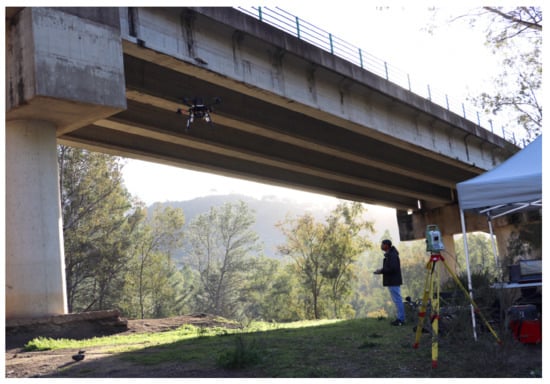
Figure 1.
Aerial robots are becoming more relevant for industrial applications in GNSS-denied or GNSS-degraded environments.
There are numerous algorithms used for localizing ground robots in an efficient and robust manner [5,6]. However, in the case of aerial robots, which move and operate in 3D environments, these methods imply greater computational complexity. Apart from the spatial dimensionality, drones are exposed to additional challenges as their onboard capabilities are limited in terms of payload, computational resources, and power constraints.
One approach for localizing aerial robots indoors, which is widely adopted in research activities, is the use of motion capture systems. They allow very accurate tracking for a broad variety of developments [7,8]. These systems are composed of a network of cameras that are strategically positioned to provide a working volume where the aerial platform can operate. However, these systems require a direct line of sight between the tracked platform and a minimum number of cameras to guarantee good performance; hence, they are not suitable for cluttered environments or dynamic scenarios. Moreover, they are not cost-effective when scaling to bigger environments.
Vision-based approaches for robot localization are very popular because of the affordability, availability, and low weight of cameras. It is very common to find algorithms that use monocular cameras fused with inertial sensors to perform Simultaneous Localization And Mapping (SLAM) [9,10,11,12]. Drawbacks of this type of technique when applied to aerial robots are tightly related to the high-speed movements of these platforms, or when they navigate in big empty spaces such as industrial scenarios. Some authors proposed the use of stereovision or RGB-D sensors [13,14,15,16] for improving monocular approaches by adding depth measurements in the form of point clouds from the environment, but the practical range when integrating them into aerial robots is usually limited to a few meters, which could be insufficient in most industrial settings. The main problem with vision-based approaches is that they do not provide a robust solution for aerial robots, due to their low reliability in the long term, not only due to the accumulated drift but also to other factors affecting cameras, such as lighting.
LiDAR (Light Detection and Ranging) is another sensing alternative to generate localization solutions based on point clouds. This research line has attracted a lot of attention recently, especially in the automotive sector [17]. There are existing algorithms that can be used for computing odometry and mapping from LiDAR data [18,19]. Their limitations arise when integrating such approaches into aerial robots, due to the presence of vibrations and/or fast motions, which could generate drift that prevents the system from being robust in the long term.
Another family of approaches that cope with long-term localization solutions relies on previously built maps of the environment, taking advantage of the fact that industrial applications usually take place in a specific setting. In addition, map-based approaches for localization are usually better in terms of reliability and computational requirements. The map can be computed offline using cameras and/or depth sensors, making use of existing algorithms. Monte Carlo localization (MCL) is an approach that makes use of a known map of the environment, commonly used for robot navigation in indoor environments [20]. It is a probabilistic localization algorithm that makes use of a particle filter to estimate the pose of the robot within the map, based on sensor measurements. Important benefits include the possibility of accommodating arbitrary sensor characteristics, motion dynamics, and noise distributions. There is an adaptive version of MCL, AMCL, which evaluates and adapts the number of particles for improving the computational load. An open-source version of AMCL is available in the Robot Operating System (ROS) (http://wiki.ros.org/amcl (accessed on 26 April 2021)); however, it is meant for wheeled robots moving in a 2D environment, requiring a 2D laser scanner for map building and localization. Other authors have proposed the use of 3D LiDAR data in MCL, but simplifying the 3D scans as 2D slices for autonomous ground vehicles [21]. To the best of our knowledge, there is no AMCL solution specifically designed for aerial robots.
Localization based on radio beacons has also been deeply studied in the last few years [22]. Radiofrequency sensors provide point-to-point distance measurements and offer a low-cost solution that can be applied in almost any scenario, with the advantage that a direct line of sight is not required between each pair of sensors. Ultra-wide band (UWB) is a wireless communication technology that has attracted the interest of the research community as a promising solution for accurate localization and tracking of targets. It is particularly suitable for applications in GNSS-denied environments, using several fixed sensors placed at known positions in the environment, plus a sensor onboard the aerial robot [23,24]. Nevertheless, these sensors are not suitable for constituting a complete localization system, due to the lack of orientation information, which leads to multiple localization hypotheses.
The aforementioned approaches are promising in the sense that they can all provide solutions to the localization problem, but there are major drawbacks if they are used separately. The presented work builds on previous research from the authors [25], a multi-modal sensor fusion approach which is based on an enhanced MCL algorithm that integrates an odometry source for short-term estimations with other sources of 3D measurements, namely 3D point clouds of the environment, a previously built 3D map, and radio-based sensors installed in the environment and localized within such a 3D map. The main contribution of the presented work focuses on a similar combination of technologies, but with a stronger focus on achieving higher accuracy and robustness for the safe introduction of aerial robots in industrial applications, thanks to the use of a 3D LiDAR sensor. To understand the improvement related to the change of sensor, Table 1 can be observed. It must be taken into account that the environment where the algorithm is intended to be applied will make it more meaningful to use one sensor or another. In our case, an industrial environment involves very wide spaces, so the range is decisive. The sensor change also makes sense in the field of precision, since it is evident that the algorithm will provide better results when the inputs on which it acts are more precise.

Table 1.
Sensor comparison.
The code and associated documentation have been published as an ROS package, publicly available at http://wiki.ros.org/amcl3d (accessed on 26 April 2021). Apart from releasing the code, a dataset including several flights with associated ground truth has been also published, so that the scientific community can benefit from our research.
Section 2 explains the details of the algorithm, as well as the aerial robotic platform that we have designed. In Section 3, the experiments performed to validate the algorithm are explained. Section 4 discusses the use of the algorithm and proposes interesting avenues for future work that could be worth exploring.
2. Materials and Methods
This section introduces the details of the algorithm developed and adapted to introduce aerial robots into industrial applications. Firstly, the designed hardware architecture is presented; later, the software is explained in detail.
2.1. Platform Description
The hardware architecture of our research platform is presented in Figure 2. The aerial robot is based on the standard DJI Matrice 600 platform, in which all sensors and the processing computer are embedded. The autopilot is DJI A3, for which a specific connection with the onboard computer was devised. We used a Ubiquiti Bullet radio device for communications between the aerial robot and the ground station. For data processing, an Intel NUC with an i7 processor was used.
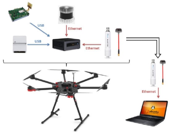
Figure 2.
Hardware architecture.
A 3D LiDAR sensor was used to obtain point clouds of the aerial robot environment. The 64-channel Ouster OS1 sensor was chosen, which counts with a vertical field of view of 45 degrees, and a range of around 100 m. However, due to the high computational load of point cloud processing, it was decided to decrease the number of scans and use only 16 channels, thus enabling greater computational efficiency. This LiDAR sensor was used for building the 3D map of the environment and for point cloud matching during the flights.
Finally, the radio sensors that were used to obtain distance measurements to and from the aerial robot were the standard model of the swarm bee ER family from Nanotron. One of them was integrated onboard the aerial robot, while the rest of the sensors were rigidly attached to different locations in the environment to serve as beacons. The accuracy of the distance measurements was 10 cm between 0 and 50 m, which was well suited to our application.
2.2. MCL Algorithm
As previously stated, our algorithm is based on a Monte Carlo localization algorithm that was previously developed by the authors [25], which was based on an RGB-D camera as the main sensor for obtaining 3D point clouds of the environment. Taking into account the redesign of the aerial robot and the new tentative applications for industrial scenarios, there are several differences. The odometry input for the particle filter is no longer based on vision but on LiDAR. The 3D point clouds that the robot acquires are very different from the ones acquired by an RGB-D camera since now they have less density and a higher range. In essence, the filter behavior is similar: it compares the map point cloud with the robot point clouds, taking also into account the radio-based measurements, to compute the weights of particles. In such an environment, the particles have different weights according to each computed probability, so the weighted average of all particles would give the estimated current robot pose (position and orientation).
Each particle i has its pose and an associated weight as follows:
where x, y, and z represent the particle position, and the yaw orientation.
The main algorithm is shown in Figure 3, and the three main parts of the particle filter loop of our implementation are explained below.
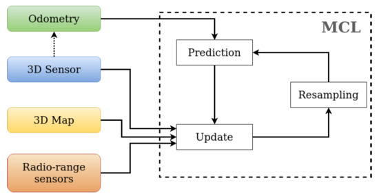
Figure 3.
Complete scheme of the algorithm.
Prediction is responsible for moving the particles according to the increment of odometry in the time interval. Thus, it generates the new particles at time according to the pose (position and yaw angle) indicated by the current aerial robot pose at time t:
The update is responsible for computing the weights of each particle . It verifies the correctness of the pose of each particle by using the 3D point cloud from the LiDAR and the radio-based measurements of the UWB sensors. The weight is calculated by using the LiDAR sensor and the map of the environment provided as an input to the algorithm. The goal is to see how well the point cloud provided by the sensor aligns to the map from each particle pose. It should be noted that an initial grid of the input 3D map is created at the beginning, as an efficient measure to reduce the run time of the algorithm. On the other hand, there is the weight that involves the radio sensors installed in the environment, whose positions are known. This weight represents how well each particle pose accommodates the received radio-based distance measurements from the UWB sensor onboard the aerial robot to the fixed sensors . This weight represents how well each particle pose fits the radio-based distance measurements received from the UWB sensor on board the aerial robot to the fixed sensors using a Gaussian distribution (mean and standard deviation where k is the corresponding beacon). Additionally, there is a parameter that is used to assign higher or lower relative importance to each of the two sensing modalities, according to the particularities of the scenario; for example, in environments with a high density of metallic structures, it is likely that radio sensors provide a higher number of incorrect distance measurements.
Lastly, the resample step is responsible for suppressing the particles that have lower values of weight and generate more particles from the ones with higher weights. Thanks to this step, the algorithm is able to converge to the correct aerial robot pose.
3. Results
3.1. Test Scenario
The environment used for validating our algorithm is in the CATEC (Advanced Center for Aerospace Technologies) facilities, which contain an indoor multi-vehicle aerial testbed (see Figure 4). This space enables the development and testing of different algorithms applied to multiple aerial platforms. The testbed dimensions are 15 m × 15 m × 5 m. It has a motion capture system based on 20 Vicon cameras, which allow the control of the full volume through the use of passive markers that are placed on the aerial robot. This system can provide, in real time, the position and attitude of the aerial vehicle with millimeter precision. The sample rate of data acquisition for our experiments was 100 Hz, enough for acquiring a high-quality ground truth for evaluating localization algorithms.
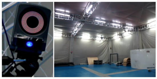
Figure 4.
Vicon camera (left) and CATEC indoor testbed (right).
3.2. 3D Map
Our enhanced MCL algorithm relies on a previously built multi-modal map that includes 3D occupancy data and the location of the UWB beacons. In this case, we built the map using Octomap [26]. A manual flight was carried out, and the aerial robot’s pose from the testbed’s motion capture system was used to project each of the 3D LiDAR point clouds onto an Octomap server, to generate the full 3D occupancy grid of the robot environment, as shown in Figure 5.
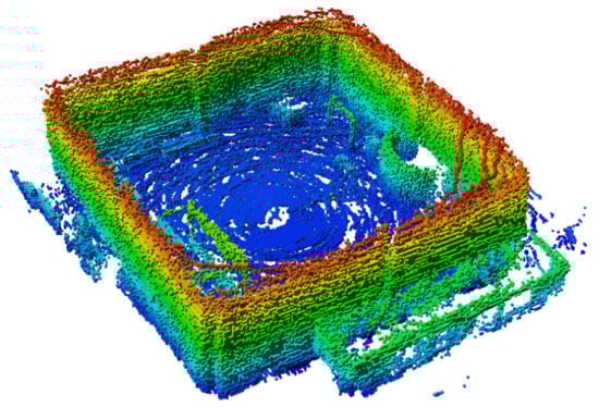
Figure 5.
Three-dimensional map of the indoor testbed at CATEC.
3.3. Public Dataset
Given the relevance of the application of aerial robots in industrial applications and the development of GNSS-free localization algorithms suitable for aerial robots, we find it necessary to provide a benchmark to test and improve them. Obtaining data from 3D LiDAR sensors mounted on aerial robots is not straightforward, and associating these data with an accurate ground truth is very relevant for the research community. This is due to the fact that this type of sensor is expensive, in addition to the need to have a multirotor capable of supporting its weight. If, in addition, the consideration of adding a ground truth is taken into account, the cost would increase even more due to the need to have a motion capture system, but it is very useful to obtain real comparisons of the resulting algorithms. For this reason, the flights used for this work have been released, thus contributing to the scientific community (see Figure 6 for a sample flight trajectory). All the published datasets can be found at: https://github.com/fada-catec/amcl3d/releases (accessed on 26 April 2021).
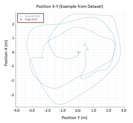
Figure 6.
Sample trajectory from one of the published flights.
3.4. Flight Test
Out of the intensive validation campaign that was carried out at the indoor testbed, in this section, we present the results from one of the most relevant flights, to show the performance of the localization algorithm. Since the robot odometry was beyond the scope of our work, we decided to use the ground truth localization but degraded it by adding a drift in position (see Figure 7-up), in order to highlight the benefits of our algorithm. In this way, it is possible to verify that the algorithm compensates for this drift and can estimate the correct pose of the robot thanks to the robust multi-sensor fusion.
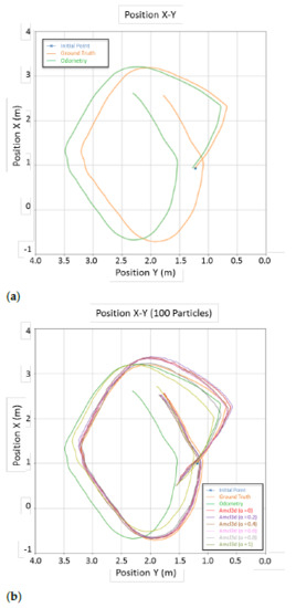
Figure 7.
(a) Input odometry with artificial drift. (b) Results provided by the algorithm in XY.
To check the possible variants of our multi-sensor fusion approach, several possibilities have been considered by modifying the parameter defined in Section 2. If this parameter is zero, only UWB measurements are taken into account, while if the value is one, only 3D point clouds are considered for weight computations. We have run the algorithm while varying this parameter with a step of 0.2, as shown in Figure 7 below.
Another variation that was tested in the algorithm was the effect of different numbers of total particles to be used. Figure 8 and Figure 9 show the errors in each state vector component (x, y, z, and ) when 100 particles and 500 particles are used, respectively. In addition, Table 2 and Table 3 provide the RMS values.
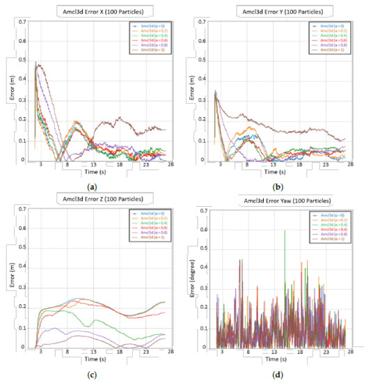
Figure 8.
Error plots using 100 particles: (a) errors in X, (b) errors in Y, (c) errors in Z, (d) errors in yaw.
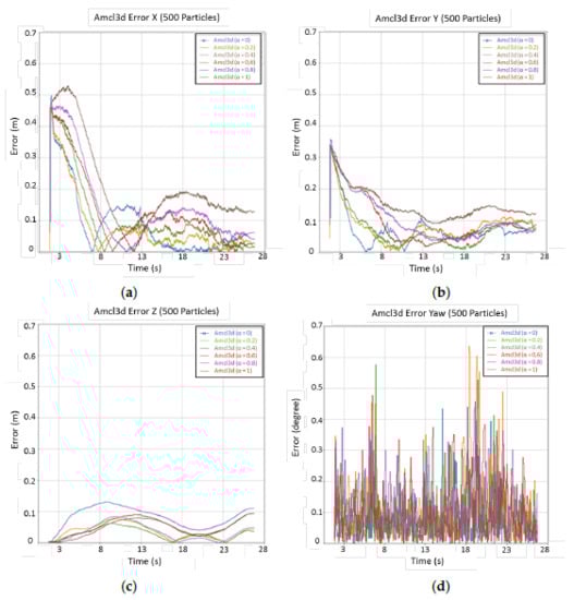
Figure 9.
Error plots using 500 particles: (a) errors in X, (b) errors in Y, (c) errors in Z, (d) errors in yaw.
Table 2.
RMS errors with different values of using 100 particles.
Table 3.
RMS errors with different values of using 500 particles.
Table 4 shows the computation load of the onboard i7 processor at different times during the test flight. As expected, there is an increase when using 500 particles, but this is not proportional to the additional amount of particles. To visually observe the progress of the computational load along the evolution of the algorithm, Figure 10 is provided.
Table 4.
Computational load with during the test execution
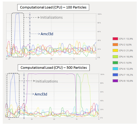
Figure 10.
Computational load graph.
The results show that our proposed algorithm can accurately locate an aerial robot in a GNSS-denied environment, even by introducing drift in the input odometry. The expected results were that the higher the number of particles, the better the results in terms of accuracy. According to Table 2 and Table 3, this would not be entirely true. Such tables take into account the whole flight, and at the beginning of the flight, the particle cloud is scattered; hence, errors are higher. The algorithm converges faster to the true pose when more particles are used, as can be seen in Figure 8 and Figure 9. It can be noted that the errors are smaller by the end of the flight, especially in the Z axis.
Therefore, it is worth comparing it with the algorithm proposed in [25]. For this reason, both Table 5 with the RMS values and the corresponding Figure 11 with the flight performed are attached. As can be observed, there is an improvement in the location in all axes and in the yaw.
Table 5.
RMS errors with MCL [25].
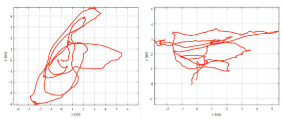
Figure 11.
Flight of [25].
4. Conclusions
Based on the results, it can be concluded that the algorithm fulfills its goals in terms of accuracy and computational efficiency. The proposed multi-sensor fusion approach provides a good trade-off, allowing variation of the proportional weight between the use of the different available sensor modalities. As for the UWB sensors, it is necessary to emphasize that the more sensors there are in the environment, the better the accuracy of the pose estimation; however, this would involve infrastructure maintenance issues for a permanent localization solution in any given scenario.
It may be of interest to the scientific community to try to locate the UAV without indicating an initial starting point. However, aerial robots perform rapidly changing movements thanks to their 6 degrees of freedom. This means that when the algorithm tries to locate the robot in a certain position, it is already in a different one. There are “jumps” in the estimation of the robot’s position that cause the algorithm to not converge correctly. Therefore, this type of algorithm is not prepared for the first initialization step to be performed automatically; that is, it is necessary to enter an initial position so that the convergence is adequate in real time and the pose of the aerial robot can be correctly estimated.
Even though technological equipment has greatly advanced in recent years and allows the processing of units with higher computational capabilities, aerial robots’ payload is still a limiting factor that needs to be addressed when it comes to onboard real-time computations.
Further research directions involve the use of additional sensors in the particle filter, such as a laser altimeter to keep the height estimation errors bounded, which are critical for the safe operation of aerial robots. Furthermore, additional improvements can be addressed within the algorithm, such as a more efficient resampling method. Nevertheless, the proposed method has been validated in a realistic indoor scenario as a suitable localization algorithm for the localization of aerial robots in GNSS-denied environments.
Author Contributions
Conceptualization, F.J.P.-G.; Data curation, P.C.; Funding acquisition, A.V.; Investigation, P.C., F.C. and R.C.; Methodology, F.C.; Project administration, F.J.P.-G. and A.V.; Software, P.C., F.C. and R.C.; Supervision, F.C. and F.J.P.-G.; Validation, P.C.; Writing—original draft, P.C. All authors have read and agreed to the published version of the manuscript.
Funding
This work was partially funded by ROSIN, a European Union H2020 project, under grant agreement no. 732287, the DURABLE project (financed by Interreg Atlantic Area Programme through the ERDF from the EC), and the PILOTING H2020 project, under grant agreement no. 871542.
Institutional Review Board Statement
Not applicable.
Informed Consent Statement
Not applicable.
Data Availability Statement
Publicly available datasets were analyzed in this study. This data can be found here: https://github.com/fada-catec/amcl3d/releases (accessed on 26 April 2021).
Conflicts of Interest
The authors declare no conflict of interest.
Sample Availability
The ROS package is avaliable at https://github.com/fada-catec/amcl3d (accessed on 26 April 2021), with corresponding documentation at http://wiki.ros.org/amcl3d (accessed on 26 April 2021). See video available at https://www.youtube.com/watch?v=Dn6LxH-WLRA (accessed on 26 April 2021).
Abbreviations
The following abbreviations are used in this manuscript:
| 2D | Two-dimensional |
| 3D | Three-dimensional |
| AMCL | Adaptive Monte Carlo localization |
| GNSS | Global Navigation Satellite System |
| IMU | Inertial Measurement Unit |
| LIDAR | Light Detection and Ranging |
| MCL | Monte Carlo localization |
| RGB | Red, Green, Blue |
| RGB-D | Red, Green, Blue-Depth |
| ROS | Robot Operating System |
| UWB | Ultra-wide band |
| UAV | Unmanned aerial vehicle |
References
- Vaidya, S.; Ambad, P.; Bhosle, S. Industry 4.0—A glimpse. Procedia Manuf. 2018, 20, 233–238. [Google Scholar] [CrossRef]
- Sachs, G. Drones: Reporting for Work. 2015. Available online: https://www.goldmansachs.com/insights/technology-driving-innovation/drones/ (accessed on 3 December 2020).
- Systems Engineering Society of Australia. European Drones Outlook Study. 2016. Available online: https://www.sesarju.eu/sites/default/files/documents/reports/European_Drones_Outlook_Study_2016.pdf (accessed on 3 December 2020).
- Wawrla, L.; Maghazei, O.; Netland, T. Applications of Drones in Warehouse Operations; ETH Zurich: Zürich, Switzerland, 2019. [Google Scholar]
- Marder-Eppstein, E.; Berger, E.; Foote, T.; Gerkey, B.; Konolige, K. The Office Marathon: Robust Navigation in an Indoor Office Environment. In Proceedings of the 2010 IEEE International Conference on Robotics and Automation, Anchorage, AK, USA, 3–7 May 2010; pp. 300–307. [Google Scholar]
- Montemerlo, M.; Becker, J.; Bhat, S.; Dahlkamp, H.; Dolgov, D.; Ettinger, S.; Haehnel, D.; Hilden, T.; Hoffmann, G.; Huhnke, B.; et al. Junior: The Stanford Entry in the Urban Challenge. J. Field Robot. 2008, 25, 569–597. [Google Scholar] [CrossRef]
- Michael, N.; Mellinger, D.; Lindsey, Q.; Kumar, V. The grasp multiple micro-uav testbed. IEEE Robot. Autom. Mag. 2010, 17, 56–65. [Google Scholar] [CrossRef]
- Perez-Grau, F.; Ragel, R.; Caballero, F.; Viguria, A.; Ollero, A. Semi-Autonomous Teleoperation of UAVs in Search and Rescue Scenarios. In Proceedings of the 2017 International Conference on Unmanned Aircraft Systems (ICUAS), Miami, FL, USA, 13–16 June 2017; pp. 1066–1074. [Google Scholar]
- Leutenegger, S.; Lynen, S.; Bosse, M.; Siegwart, R.; Furgale, P. Keyframe-based visual-inertial odometry using nonlinear optimization. Int. J. Robot. Res. 2015, 34, 314–334. [Google Scholar] [CrossRef]
- Forster, C.; Zhang, Z.; Gassner, M.; Werlberger, M.; Scaramuzza, D. SVO: Semidirect visual odometry for monocular and multicamera systems. IEEE Trans. Robot. 2016, 33, 249–265. [Google Scholar] [CrossRef]
- Qin, T.; Li, P.; Shen, S. Vins-mono: A robust and versatile monocular visual-inertial state estimator. IEEE Trans. Robot. 2018, 34, 1004–1020. [Google Scholar] [CrossRef]
- Sumikura, S.; Shibuya, M.; Sakurada, K. OpenVSLAM: A Versatile Visual Slam Framework. In Proceedings of the 27th ACM International Conference on Multimedia, Nice, France, 21–25 October 2019; pp. 2292–2295. [Google Scholar]
- Schmid, K.; Tomic, T.; Ruess, F.; Hirschmüller, H.; Suppa, M. Stereo Vision Based Indoor/Outdoor Navigation for Flying Robots. In Proceedings of the 2013 IEEE/RSJ International Conference on Intelligent Robots and Systems, Tokyo, Japan, 3–7 November 2013; pp. 3955–3962. [Google Scholar] [CrossRef]
- Endres, F.; Hess, J.; Sturm, J.; Cremers, D.; Burgard, W. 3-D Mapping with an RGB-D Camera. IEEE Trans. Robot. 2014, 30, 177–187. [Google Scholar] [CrossRef]
- Mur-Artal, R.; Tardós, J.D. Orb-slam2: An open-source slam system for monocular, stereo, and rgb-d cameras. IEEE Trans. Robot. 2017, 33, 1255–1262. [Google Scholar] [CrossRef]
- Labbé, M.; Michaud, F. RTAB-Map as an open-source lidar and visual simultaneous localization and mapping library for large-scale and long-term online operation. J. Field Robot. 2019, 36, 416–446. [Google Scholar] [CrossRef]
- Wolcott, R.W.; Eustice, R.M. Robust LIDAR localization using multiresolution Gaussian mixture maps for autonomous driving. Int. J. Robot. Res. 2017, 36, 292–319. [Google Scholar] [CrossRef]
- Zhang, J.; Singh, S. LOAM: Lidar Odometry and Mapping in Real-time. In Proceedings of the Robotics: Science and Systems X. Robotics: Science and Systems Foundation, Berkeley, CA, USA, 12–16 July 2014. [Google Scholar] [CrossRef]
- Shan, T.; Englot, B.; Meyers, D.; Wang, W.; Ratti, C.; Rus, D. LIO-SAM: Tightly-coupled Lidar Inertial Odometry via Smoothing and Mapping. arXiv 2020, arXiv:2007.00258. [Google Scholar]
- Thrun, S.; Fox, D.; Burgard, W.; Dellaert, F. Robust Monte Carlo localization for mobile robots. Artif. Intell. 2001, 128, 99–141. [Google Scholar] [CrossRef]
- Wan, G.; Yang, X.; Cai, R.; Li, H.; Zhou, Y.; Wang, H.; Song, S. Robust and Precise Vehicle Localization Based on Multi-Sensor Fusion in Diverse City Scenes. In Proceedings of the 2018 IEEE International Conference on Robotics and Automation (ICRA), Brisbane, Australia, 21–25 May 2018; pp. 4670–4677. [Google Scholar]
- Fabresse, R.F.; Caballero, F.; Maza, I.; Ollero, A. Robust Range-Only SLAM for Unmanned Aerial Systems. J. Intell. Robot. Syst. 2015, 84. [Google Scholar] [CrossRef]
- González-Jiménez, J.; Blanco, J.L.; Galindo, C.; Ortiz-de Galisteo, A.; Fernández-Madrigal, J.A.; Moreno, F.; Martínez, J. Mobile robot localization based on Ultra-Wide-Band ranging: A particle filter approach. Robot. Auton. Syst. 2009, 57, 496–507. [Google Scholar] [CrossRef]
- Tiemann, J.; Schweikowski, F.; Wietfeld, C. Design of an UWB Indoor-Positioning System for UAV Navigation in GNSS-Denied Environments. In Proceedings of the 2015 International Conference on Indoor Positioning and Indoor Navigation (IPIN), Banff, AB, Canada, 13–16 October 2015; pp. 1–7. [Google Scholar]
- Perez-Grau, F.; Caballero, F.; Viguria, A.; Ollero, A. Multi-sensor three-dimensional Monte Carlo localization for long-term aerial robot navigation. Int. J. Adv. Robot. Syst. 2017, 14. [Google Scholar] [CrossRef]
- Hornung, A.; Wurm, K.M.; Bennewitz, M.; Stachniss, C.; Burgard, W. OctoMap: An Efficient Probabilistic 3D Mapping Framework Based on Octrees. Auton. Robot. 2013, 34, 189–206. [Google Scholar] [CrossRef]
Publisher’s Note: MDPI stays neutral with regard to jurisdictional claims in published maps and institutional affiliations. |
© 2021 by the authors. Licensee MDPI, Basel, Switzerland. This article is an open access article distributed under the terms and conditions of the Creative Commons Attribution (CC BY) license (https://creativecommons.org/licenses/by/4.0/).