Real UAV-Bird Image Classification Using CNN with a Synthetic Dataset

Abstract

A large amount of training image data is required for solving image classification problems using deep learning (DL) networks. In this study, we aimed to train DL networks with synthetic images generated by using a game engine and determine the effects of the networks on performance when solving real-image classification problems. The study presents the results of using corner detection and nearest three-point selection (CDNTS) layers to classify bird and rotary-wing unmanned aerial vehicle (RW-UAV) images, provides a comprehensive comparison of two different experimental setups, and emphasizes the significant improvements in the performance in deep learning-based networks due to the inclusion of a CDNTS layer. Experiment 1 corresponds to training the commonly used deep learning-based networks with synthetic data and an image classification test on real data. Experiment 2 corresponds to training the CDNTS layer and commonly used deep learning-based networks with synthetic data and an image classification test on real data. In experiment 1, the best area under the curve (AUC) value for the image classification test accuracy was measured as 72%. In experiment 2, using the CDNTS layer, the AUC value for the image classification test accuracy was measured as 88.9%. A total of 432 different combinations of trainings were investigated in the experimental setups. The experiments were trained with various DL networks using four different optimizers by considering all combinations of batch size, learning rate, and dropout hyperparameters. The test accuracy AUC values for networks in experiment 1 ranged from 55% to 74%, whereas the test accuracy AUC values in experiment 2 networks with a CDNTS layer ranged from 76% to 89.9%. It was observed that the CDNTS layer has considerable effects on the image classification accuracy performance of deep learning-based networks. AUC, F-score, and test accuracy measures were used to validate the success of the networks.

1. Introduction

The usage of commercial unmanned aerial vehicles (UAVs) has been increasing recently [1]. The identification and detection of UAVs is important for the security measures of airports, military zones, personal private zones, and human life and privacy [2]. UAVs are classified as either fixed-winged unmanned aerial vehicles (FW-UAV) or rotating-wing unmanned aerial vehicles (RW-UAV). FW-UAVs are both harder to pilot and more costly than RW-UAVs. In additional, FW-UAVs require a runway for landing and departure, whereas RW-UAVs can take-off and land on an area of 1 m². As a result of these advantages, RW-UAVs are more commonly used and outnumber FW-UAVs [1]. For these reasons, it is important to detect RW-UAVs with easily accessible sensors such as cameras for privacy and security.

Several RW-UAV detection and identification studies can be found in the literature. Radar, voice recognition, and image recognition-based methods or hybrid systems [3] have been used for detection and identification purposes. The above-mentioned radar, voice, and image-based UAV detection methods utilize antenna, microphone array, and camera hardware, respectively. Machine learning (ML) methods are among the most frequently used methods to classify UAVs with sensor fusion data. Image classification methods with artificial intelligence (AI) are used in UAV classification studies [3]. Image classification methods with AI consist of a series of processes such as data collection, data preparation and labeling, training, and testing [4]. The data type for training ML models in image classification problems is image. Data collection and data preparation are accomplished by taking photos of the relevant class or by collecting and screening from the Internet; later, they are labeled individually by hand [5]. The process of collecting the data, such as images, radar fingerprints, or voice fingerprints, that are required for ML model training is labor-intensive and time-consuming. In the RW-UAV detection process, it is important to identify birds that are likely to be in the sky, as well to avoid any confusion in application. Therefore, a labeled dataset should consist of the image classes of birds and RW-UAVs to develop a successful ML identification model that can classify birds and RW-UAVs. The methods used to create a dataset include ready-made datasets such as IMAGENET [6] and CIFAR10 [7], or photographing objects at different angles for classes without datasets.

The collection of data and the arrangement of these collected data according to the ML model is called data collection and preparation, which is a preliminary process for training. The accuracy rate is measured in the test process of the ML model, and the training process is completed using the dataset of the specified classes. Data collection and data preparation processes are labor-intensive, creating a significant workload that is repeated for each new class when training the ML model [8]. More recently, the success of image classification research has increased with the development of deep learning-based ML models. Classical ML techniques include operations such as feature extraction and selection. Feature extraction and selection layers are manual processes in classical ML, and these layer requirements have been automated in ML models based on deep learning (DL) [9]. The automation of these layers can be considered to be an advantage of DL networks; however, this advantage has the disadvantage that DL networks require more training data [10]. The most-used method in deep learning-based image classification studies is the convolutional neural network (CNN). CNN with deep learning-based networks is a rapidly developing technology, and is becoming a more widespread method for image data-type classification studies [11]. The best-known image classification competition in recent years is the IMAGENET large-scale visual recognition challenge (ILSVRC). The highest-ranked participants used CNN-based methods in ILSVRC [6]. CNN networks consist of two core structures, called the convolution and pooling layers. The convolution layer consists of feature maps, with each connected to each other and consisting of a series of weights, and eventually connects to a function such as a rectified linear unit (RELU).

Networks frequently used in image classification studies with CNN are AlexNet, Visual Geometry Group Network (VGGNet), and SqueezeNet architectures. There are studies that have achieved RW-UAV and bird image classification by using deep learning-based architectures [12]. The image data used for training and testing in these studies consist of real photographs that were taken manually. Real photographs of objects belonging to each class must be created to train AI in the general approach to AI model training. The disadvantage of AI studies in which real photo data are used is that real data collection is a difficult and labor-intensive task. In addition, taking photos of real data is difficult depending on the outdoor environment conditions, such as altitude, danger zone, and adverse weather conditions. Considering the importance of the diversity and amount of data in AI training and the difficulty of creating a dataset manually, the following research questions need to be addressed: “Can the artificial intelligence training-image dataset be synthetically produced as needed?” and “Can an artificial intelligence model trained with synthetic data be used to classify a real-image dataset?”.

In this study, we have focused on increasing the accuracy of results obtained by trained deep learning-based ML models with a fully synthetic-image dataset and tested them with a real-image dataset. To create a synthetic dataset, a virtual studio was created by using the Unity game engine, and 69,120 synthetic images were created for bird and RW-UAV three-dimensional (3D) models. In total, 34,560 synthetic RW-UAV images and 34,560 synthetic bird images were produced, and the 216 ML models were trained with these synthetic images. Models were tested with 3385 real images and 5000 synthetic images separately.

We propose a new approach to improve the accuracy of the DL networks trained with synthetic images and tested with real images. The proposed approach, corner detection, and nearest three-point selection (CDNTS), is a hybrid method of corner detection methods and the nearest point search method for feature extraction that can be used with DL networks. Corner detection-based methods are commonly used in visual tracking [13], image matching and photography [14], robotic path finders [15], etc. This approach is a technique that is generally used to detect corners in images in image-based studies. The “nearest three-point selection” part that forms the other half of the hybrid CDNTS layer is a function that searches for the closest points. Nearest-point search problems, which basically aim to determine the distance of two or more points to each other, are a common subject of interest in the literature research studies. This approach is used to group the pixels of two-dimensional (2D) images and vertexes of 3D point cloud data and determine the closest pixels and vertexes in [16]. It is used in algorithms that form a decision tree by finding the distances between the weights of classes in decision tree problems [17]. The CDNTS layer suggested in our study can be considered to be a feature extraction technique that utilizes the “corner detection” and “nearest point search” method. The CDNTS layer consists of three main operations: corner point coordinate detection, the calculation of the distance between corners, and drawing lines between the closest three corners. As a result of these operations, the original image is transformed into an image consisting of corner points and lines. The corner detection-based CDNTS is a hybrid layer that improves the accuracy of the real-image classification of DL networks trained using synthetic images.

The performance, computation times, validations, and test accuracies of the methods were measured. The results obtained from both experimental setups were verified with the validation methods of the F-score [18] and the area under the curve (AUC). AUC and test accuracy parameters were computed to analyze the performance and success of the network. The F-score parameter is a parameter that calculates test accuracy via recall and precision.

2. Related Work

Image classification has become an active research topic in computer vision. CNN-based image classification methods play an important role in image classification. In addition, with the development of graphics processing unit (GPU)-based hardware and open source libraries such as Tensorflow [19] and Keras [20], CNN-based image classification learning algorithms have become prominent [11]. Some of the CNN-based architectures used for image classification are AlexNet [21], SqueezeNet [22], and VGG16 [23] as convolutional neural network (CNN) algorithms.

The accuracy performances of these DL algorithms may be different. In order to train a DL network for image classification, a dataset with a large number of images should be introduced to the network [9]. Some libraries such as IMAGENET [6] and CIFAR10 [7] provide picture datasets to train the network. IMAGENET and CIFAR10 libraries consist of labeled image data that are directly obtained from real picture data by photographing. This library has been used in some studies in the literature to solve some image classification problems [6,24]. Due to the fact that datasets have a limited number of classes, they might not offer solutions to all problems with a desired accuracy. To train a class that is not available in libraries, it is necessary to create a new dataset. In such cases, a dataset can be created by taking many object photographs with a camera or by generating synthetic images with a game engine [25,26] according to the problem. CNN-based algorithms are frequently used to train DL networks for image classification [27,28,29]. There are some studies in the literature which make use of CNN-based image classification using pictures of real objects or synthetic objects [30].

Several studies have used synthetic object image data to identify computer-aided design (CAD) model files provided from the CAD model library [31]. Some studies also use a video and image dataset created with the rendering tools of game engines [32,33,34] to integrate AI into the games. The common purpose of machine learning studies using synthetic data in addition to real data is to increase the number of samples of datasets where the number of samples is low or limited [32]. In cases where the number of samples is limited and a CNN-based machine learning algorithm is used, the success of the network is low. To increase the performance of the network, many samples are needed [35]. To increase the number of samples, synthetic images can be generated by using 3D models and game engines. Using a game engine’s rendering tools, a 3D model can be photographed from different angles and distances. This flexibility provided by the game engine allows the creation of many samples and removes the constraints on the dataset. In the literature, this method is used to diversify real datasets and increase the number of data. In this study, we aimed to create a dataset from fully synthetic data.

3. Materials and Methods

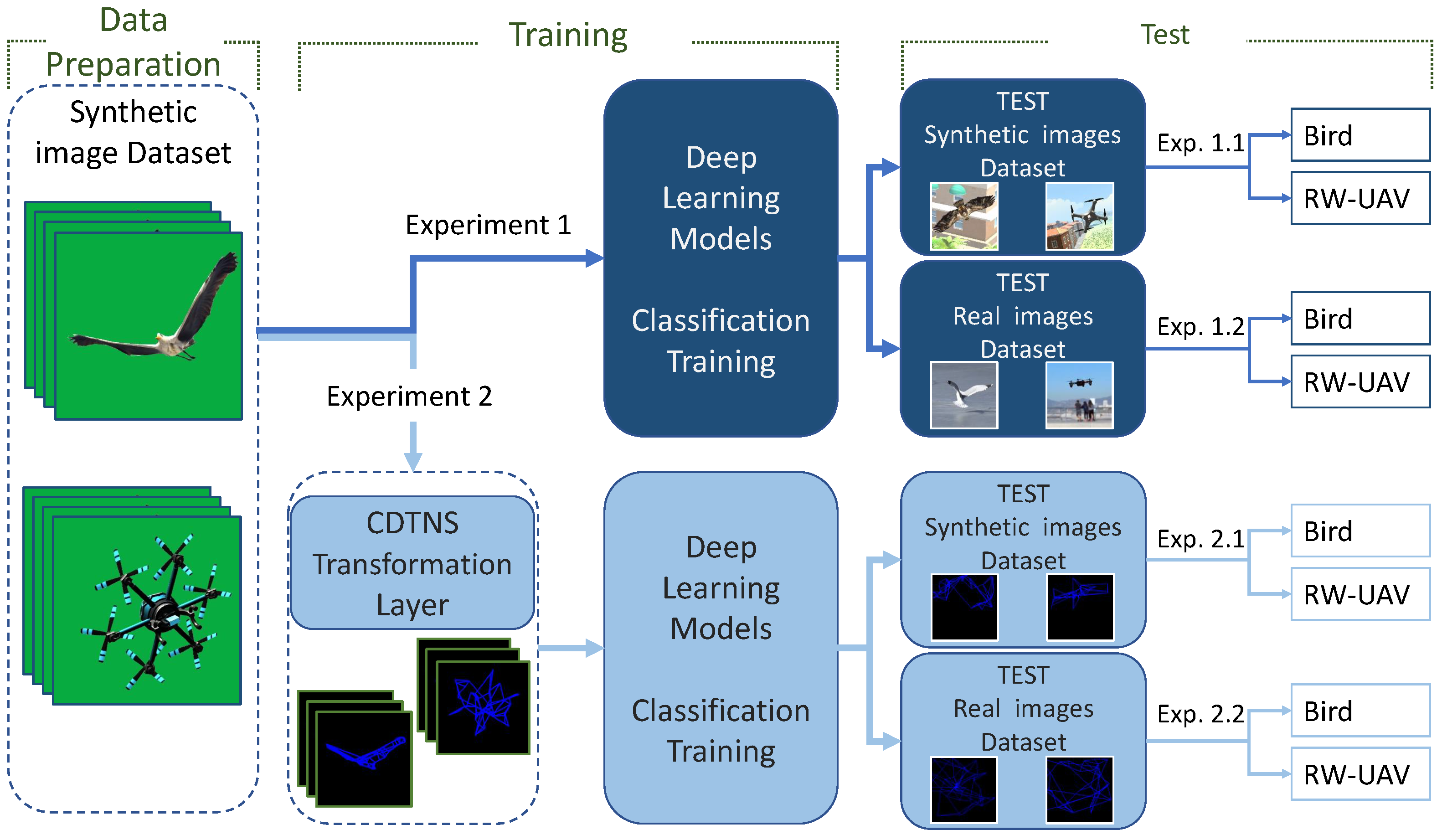
AI training using synthetic data and the test stages of the trained AI model were carried out for two experiments. The two experimental setups are shown in Figure 1.

A green box studio was created in the unity game engine where RW-UAV and bird images could be created to generate a training dataset using 3D models as desired. In total, 34,560 RW-UAV and 34,560 bird images were created using the green box studio by photographing from different angles. The created synthetic data were used as a training sample in DL networks. The AI was trained using fully segmented synthetic data. The two datasets used in the test phase consisted of non-segmented synthetic and real data. The trained AI was tested with real data and synthetic data separately. The real test data were created from images with different objects in the background. Two cities with old and modern designs were created in the unity environment to generate synthetic test data. Using images from different regions of these cities, a background was created for the test data. Real images and synthetic RW-UAV and bird images with a city background were created and tested to measure the accuracy of the trained AI model. The test data using synthetic and real data were tested and analyzed for both experiments.

3.1. Generate Synthetic Training Dataset

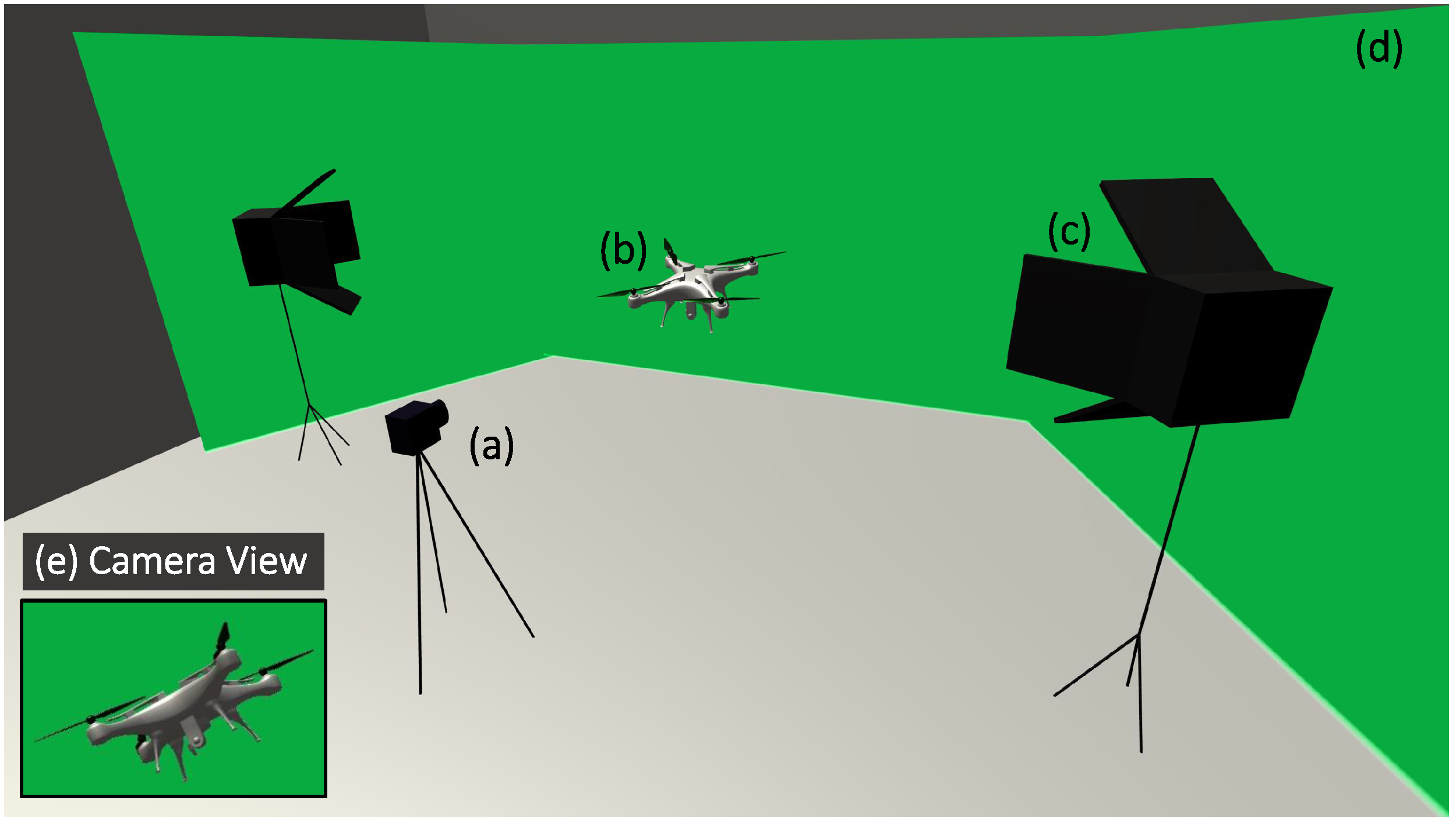
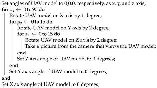
A total of 69,120 2D red–green–blue (RGB) synthetic images were created from three different RW-UAVs and three different birds in 3D models. This conversion process involved converting the 3D model file into a 2D image file by taking photos at different angles. 3D models were rotated around the X, Y, and Z axes at defined angles and photographed at every angle change as unique. In this way, the required images were created for the experimental dataset. Figure 2 shows the green box studio which was designed and created in the unity environment to photograph the models and record them as synthetic images in the segment. The background color tone chosen for the green box studio was specially selected to facilitate the background extraction process. In the process of producing all synthetic images, RW-UAV and bird model images were photographed from different angles and were uniquely produced. This uniqueness was ensure by rotating and photographing the models at a certain angle step by step on the X, Y, and Z axes by using the algorithm shown in Algorithm 1, which yielded 34,560 images for each class.

Algorithm 1: RW-UAV model rotation and synthetic image generator algorithm in the unity game engine.

Images in AI training, validation, and test dataset must be different from each other; therefore, all images were encrypted by utilizing the message-digest algorithm 5 (MD5) and compared to ensure there was no duplication. Encrypting and comparison of image files to avoid duplication is a method that used in the literature [36].

To measure the prediction success of the DL network trained with synthetic images, a different synthetic images dataset needed to be created. The images involved in the network’s training and testing processes must be different from each other. This uniqueness is necessary for the reliability of experiments. A simulation environment that occurs from modern and old city designs was created within the unity game engine to test the network’s predictability in daily life. This simulation environment was created for two different cities that have lakes, forest, and buildings; in addition, our designs reflected historical and modern style perspectives. These cities were created with models purchased from the unity asset store [37].

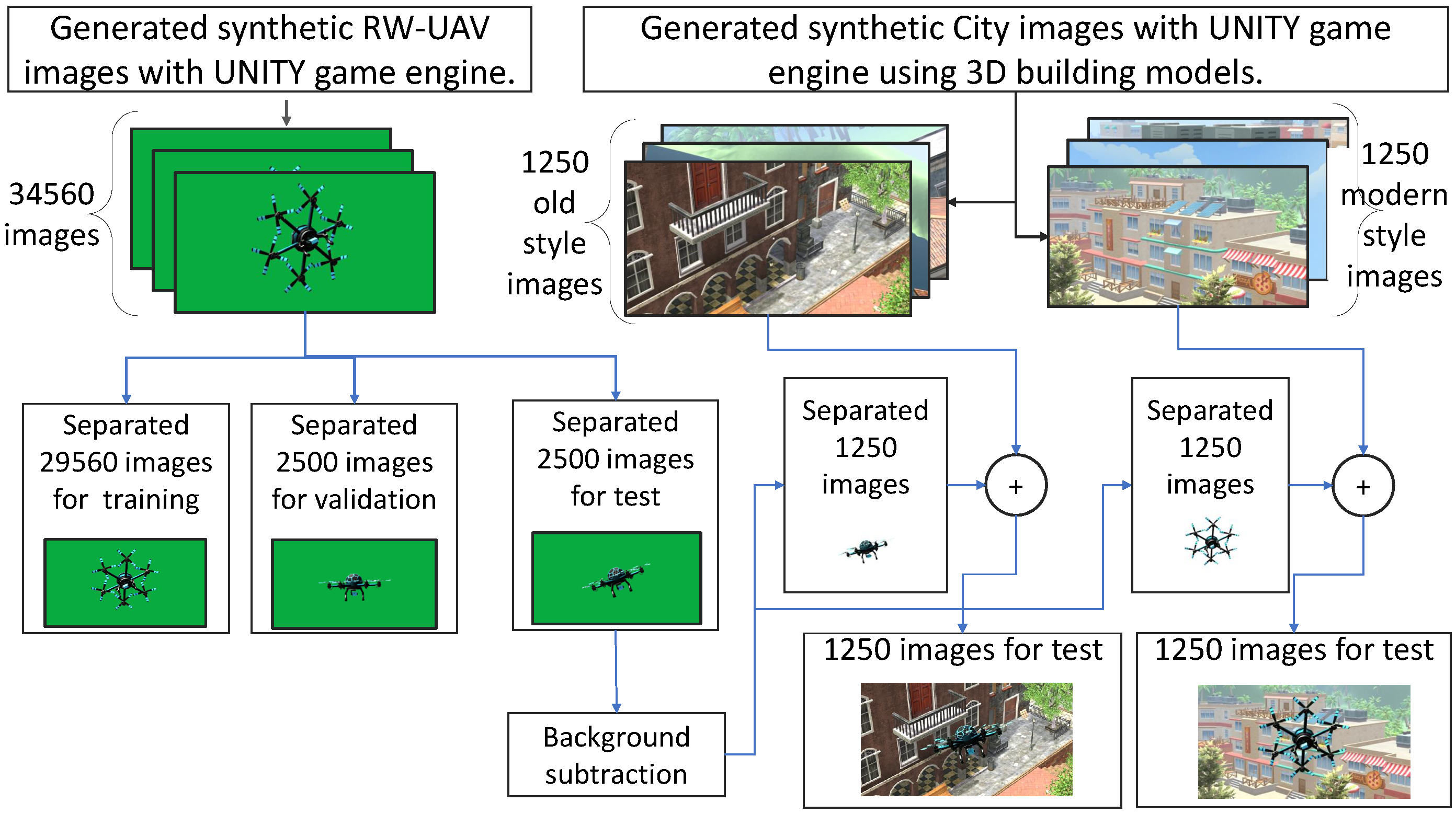
An image of two cities from different angles are shown in Figure 3. Images generated in the green box were divided into three groups: validation, training, and test stages. The background for the test data was green. The green color was extracted from the background of the synthetic test data, and city images were inserted instead. The dataset preparations for the test and training data are shown schematically in Figure 4. The schematic representation related to the creation of a dataset of the RW-UAV images class was applied to the creation process of the bird-images dataset.The size of all synthetically produced images was set to 224 × 224 pixels for comparison and evaluation of experiments. The 90 × 90 pixels part of these images consists of the object photograph. Therefore, RW-UAV and Bird images are a 90 × 90 pixels portion of the 224 × 224 pixels image.

3.2. Real-Test Dataset Collection and Preparation

Testing the AI with synthetic dataset after the training process was completed with synthetic data that enabled us to measure the success of the model. It was important that the AI trained with synthetic data should be tested using a real-images dataset. The dataset consisting of real images was gathered from pictures and videos available on the Internet. The real dataset was subjected to manual and software control processes to remove similar and duplicate images. The dataset creation process took place in two stages. A developed script downloaded videos from the Internet and recorded images at intervals of 5 s, and the images were downloaded by using the Google search engine. In the second step, the dataset created by the script was manually checked and extracted. In addition, by using the function named template match modes coefficients normed (TM_CCOEFF_NORMED) of the open source computer vision library (OPENCV) [38], similar images were detected and extracted by using the comparison script. The similarity extraction method is a method that has been used in the literature, and we extracted all images with a similarity rate of more than 80% [39]. The TM_CCOEFF_NORMED function is represented by Equation (1).

$$R(x,y)=\frac{{\sum }_{x^{\prime },y^{\prime }}(T^{\prime }(x^{\prime },y^{\prime })\cdot I^{\prime }(x+x^{\prime },y+y^{\prime }))}{\sqrt{{\sum }_{x^{\prime },y^{\prime }}{T}^{\prime }{(x^{\prime },y^{\prime })}^2\cdot {\sum }_{x^{\prime },y^{\prime }}{I}^{\prime }{(x+x^{\prime },y+y^{\prime })}^2}},$$

(1)

where T, R, I, and (x, y) values are the template, resulting image, source image, and position of pixel values, respectively. Using these methods, a dissimilar dataset consisting of 1859 birds and 1526 RW-UAV real images was created. Some examples of real datasets are presented in Figure 5.

The size of the real images collected were between 227 × 227 pixels and 1280 × 1280 pixels. Image sizes were scaled and converted to 224 × 224 pixels for the trained AI to make prediction. At the end of the resizing, a dataset with RW-UAV and bird image fragment size between 8 × 8 pixels and 95 × 95 pixels within a 224 × 224 pixel image was created. For a realistic test scenario, a dataset with different object size ratios between 8 × 8 pixels and 95 × 95 pixels was created.The same size pictures shown in Figure 5 contain different sizes of RW-UAV and bird image fragments.

3.3. Train and Test Setup

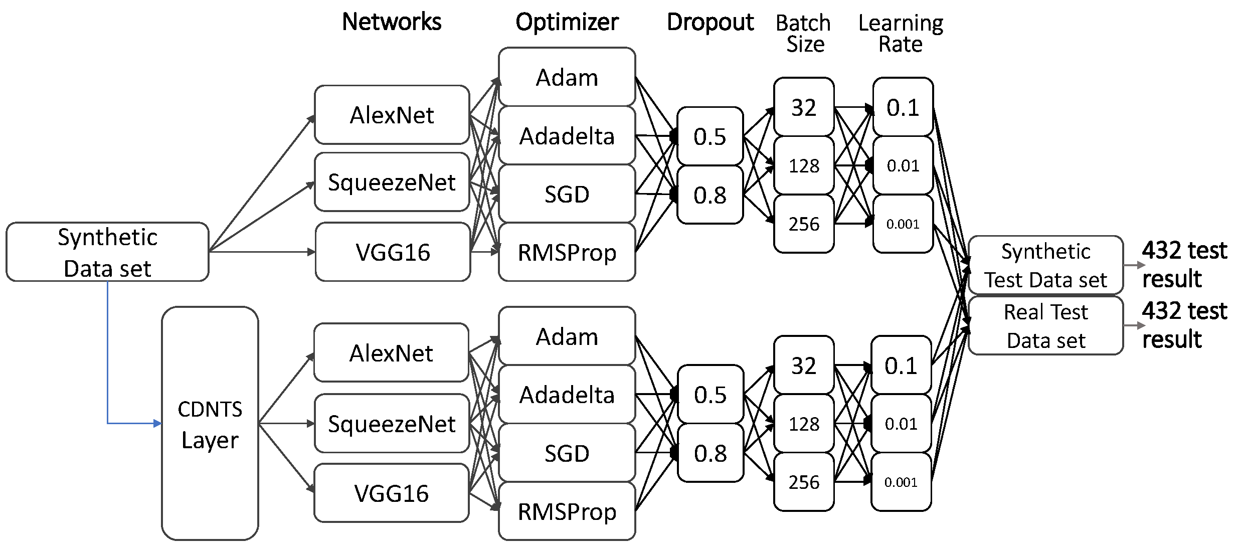
The dataset consisting of synthetic images was used to train deep learning-based classification networks—specifically AlexNet, SqueezeNet, and VGG16—in the setups for experiments 1 and 2 (see Figure 1). All combinations of AlexNet, SqueezeNet, VGG16 DL networks, and adaptive moment estimation (Adam) [40], adaptive learning rate method (AdaDelta) [41], stochastic gradient descent (SGD) [42], and root mean square error probability (RMSprop) [43] optimizers were applied for these two experiments. Networks and optimizers were trained with combinations of the different hyperparameters listed in

Table 1. The combinations of hyperparameters.

Hyperparameters	Values
Optimizers	Adam/Adadelta/RMSprop/SGD
Batch Size	32/128/256
Learning Rate	0.1/0.01/0.001
Dropout	0.5/0.8

.

In experiment 2, unlike experiment 1, a CDNTS layer was included. By comparing the results of experiments 1 and 2, the success of the CDNTS layer in the training of the network was measured and reported. The synthetic dataset created in the green box was divided into train, validation, and test sets, as shown in Figure 4. The synthetic test data background was combined with modern and old city views. Training, validation, synthetic testing, and real test data were trained, tested, and reported for four different DL networks. Deep learning-based classification networks should be selected considering their speed and accuracy [44]; therefore, in this study, we tested four different networks and compared the speeds and accuracy of the networks to present a comprehensive comparison. All training and testing stages were carried out by using the GPU computing system (GeForce GTX 1080ti, Nvidia Corp., Santa Clara, CA, ABD), 128 gigabyte (GB) random access memory (RAM), I7 processors and the TensorFlow-based [19] Keras [20] library. Experiment 2 consists of a CDNTS layer combined with deep learning-based classification methods in train and test phases. As shown in Figure 1, the synthetic training dataset was introduced to the DL networks after passing through the CDNTS layer. The F-score value and AUC metric were used to verify the classification accuracy performance of the trained AI model. The F-score (Equation (2)) was calculated alongside the precision (Equation (3)) and recall (Equation (4)).

$$F_{score}=2\cdot \frac{Precision\cdot Recall}{Precision+Recall},$$

(2)

$$Precision=\frac{TP}{TP+FP},$$

(3)

$$Recall=\frac{TP}{TP+FN},$$

(4)

where TP, TN, FP, and FN are true positives, true negatives, false positives, and false negatives, respectively.

3.4. Corner Detection and Nearest Three-Point Selection Layer (CDNTS)

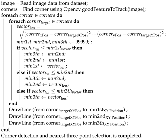
The test accuracy results of the synthetic test and real test data of the networks trained with synthetic data were measured in experiment 1. As a result of experiment 1, the accuracy of the synthetic test data was acceptable, while the accuracy of the real test data did not exceed 60%. Therefore, studies were carried out to increase the test accuracy of real test data. As a result of our investigation, the usage of a layer named CDNTS has been proposed. Some studies in the literature have shown that the choice of method for the feature extraction of images may be a successful way to improve the performance of a CNN-based algorithm [45]. Simple and lower-dimensional RW-UAV images created from lines drawn between the corner points of the images could improve the performance of DL algorithms [46]. Therefore, a layer called the corner detection and nearest three-point selection (CDNTS) layer was added to the front of the CNN-based networks. This layer, designed for the input of CNN-based networks, is an algorithm that finds corner points in the images and connects the three closest corner points with lines. The “good features to track” library of the OPENCV framework was used to detect corners. The corner detector library was developed by Shi-Tomasi with the authors in [38,47]. Position data of corner points found by the corner detector were used to draw lines between the nearest three corner points. There are studies in the literature that draw continuing lines between points [48]. In our study, the continuity of the lines drawn between the points was ignored. A line was drawn between the three closest points to each point. Algorithm 2 was generated from CDNTS algorithms. The corner detection algorithm, which is a part of the CDNTS layer, was created using the OPENCV library. Another part of the CDNTS layer, the nearest three-point selection part, was coded by the authors. A general representation of the algorithm is shown in Algorithm 2.

Algorithm 2: Corner detection and nearest three-point selection layer.

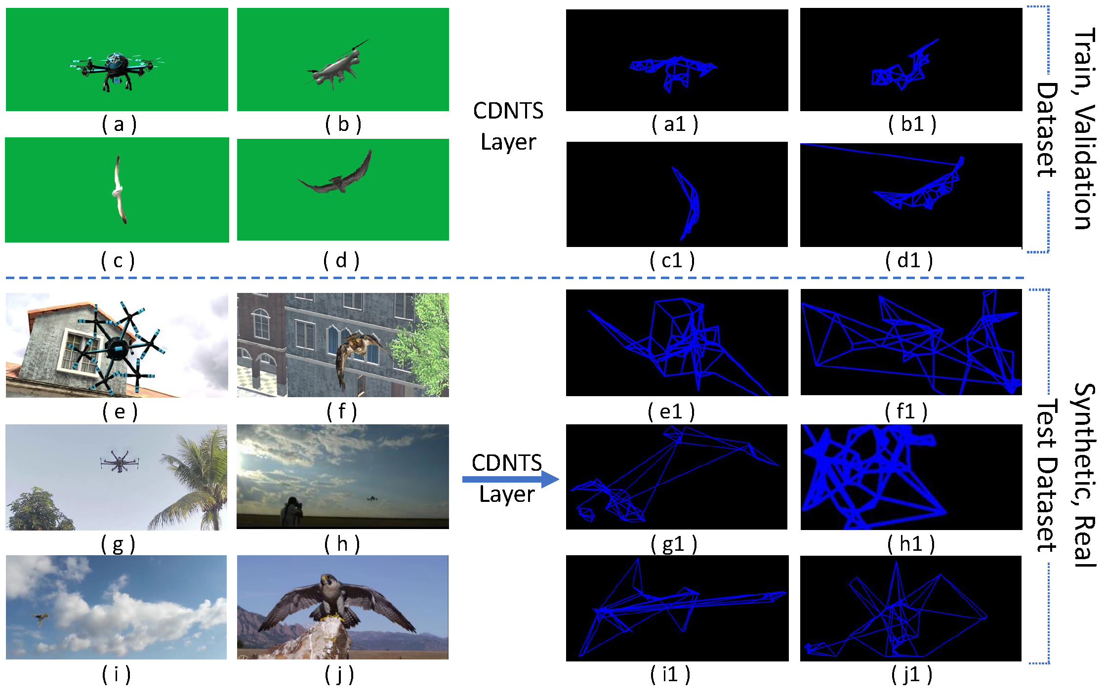
Algorithm 2 was used to find the corner points of the images and to draw a new image with lines between the three closest corner points. This new image consisting of only corners and lines was then given to the CNN-based network. Sample output images of Algorithm 2 are shown in Figure 6.

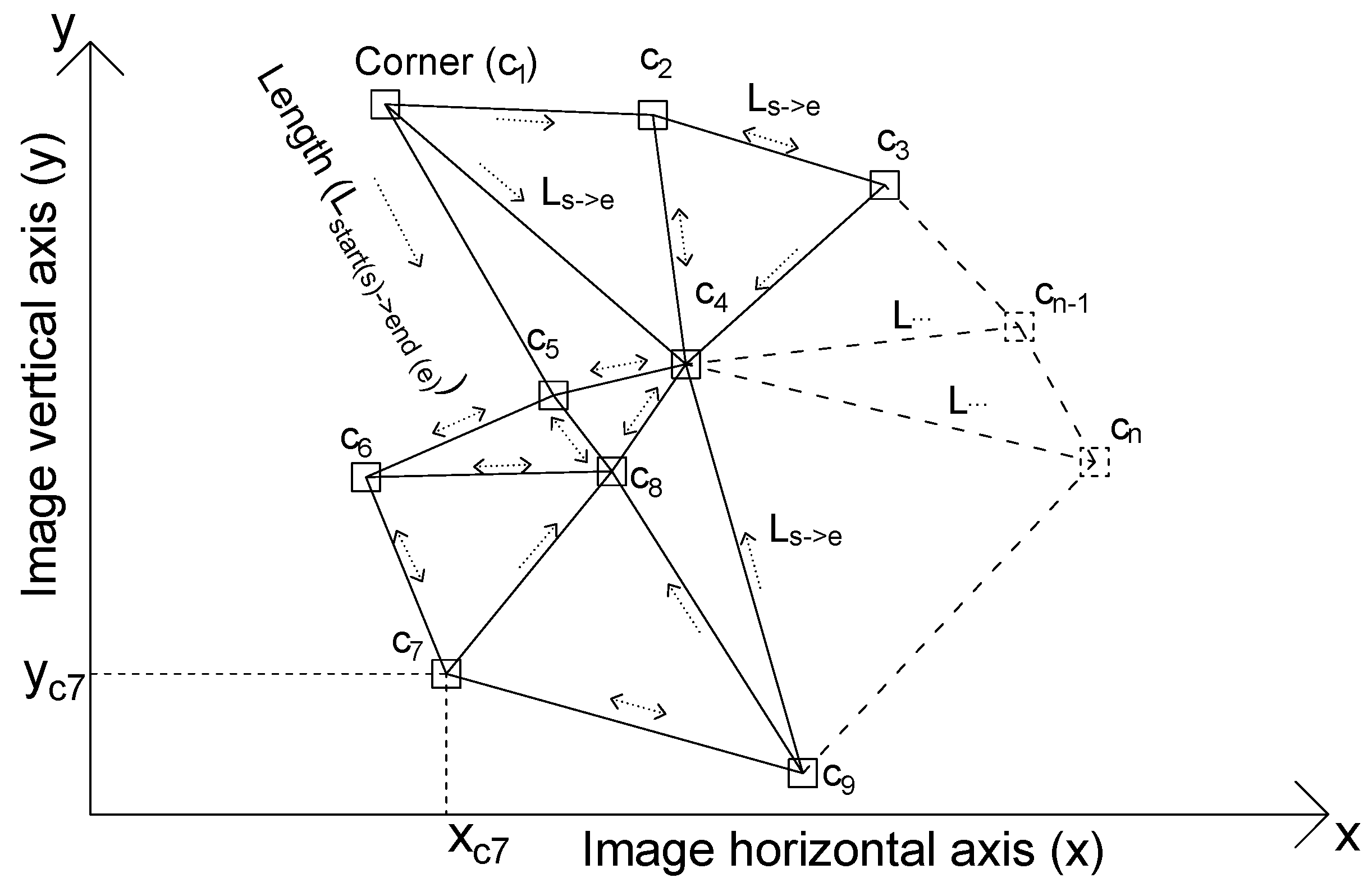
A schematic representation of the CDNTS layer nearest three-point selection process is shown in Figure 7. The letters y, x, c, and L defined on the graph refer to the image pixel vertical coordinate, image pixel horizontal coordinate, detected corner, and distance between vertices, respectively. The formula for calculating the variable L is given by Equation (5).

$$L_{c_n->c_t}=\sqrt{{(x_{cn}-x_{ct})}^2+{(y_{cn}-y_{ct})}^2},$$

(5)

where L_cn->ct, x_cn, x_ct, y_cn, and y_ct values are the vector length between selected corner and target corner, selected corner x axis position , target corner x axis position, selected corner y axis position, and target corner y axis position, respectively.

The distance calculation formula was repeated in a loop to determine the distances of all vertices to other corners. In the loop, the closest point was searched for, and a line was drawn to the nearest corner. A previously drawn line could be re-drawn in case two vertices were the nearest corners to each other. This overlap process is shown in the schematic representation with a double-sided arrow. The one-sided arrows show the starting and ending points of the lines between the corners.

4. Result and Discussion

4.1. Training and Test Results

We examined the AI training using synthetic data under two methods (experiments 1 and 2). In both methods, three different networks were trained to determine the most successful network and optimizer with a combination of four optimizers, two dropout values, three batch size values, and three learning rate values. Therefore, a total of 432 trained combinations of models were obtained, including 216 different trained models in experiment 1, and 216 different trained models in experiment 2. Experiment 1 consisted of training deep learning-based classification networks without a CDNTS layer, while experiment 2 consisted of training deep learning-based classification networks with a CDNTS layer. Each model was trained and later tested in comparison with a real-test dataset and synthetic-test dataset, and the 432 combinations are presented in Figure 8.

The test accuracy results and training accuracy results of experiments 1 and 2 were compared. It was reported in experiment 2 that the added CDNTS layer affected the training time that defined average cost of training time is 36.7 ms and 75.9 ms/image. The CDNTS layer with an attached network in experiment 2 gave improved results for real and synthetic datasets. The training models of all hyperparameter combinations were tested separately with synthetic-image and real-image test data. The results of experiments with two subtests—experiments 1.1, 1.2, 2.1, and 2.2—are reported in

Table 2. Experiment 1: Deep learning-based networks’ F-score, accuracy (Acc), and AUC values of the test results. It shows the test success of networks trained without using the CDNTS layer. Values that styled bold represent the most successful test listed. Lr: Learning Rate, Bs: Batch Size.

	Exp 1.1 Synthetic Images Test			Exp 1.2 Real Images Test
Model	F-Score	Acc	AUC	F-Score	Acc	AUC
Optimizer	(%)	(%)	(%)	(%)	(%)	(%)
AlexNet	<55	<55	<55	<55	<55	<55
for All	Lr: for all, Bs: for all			Lr: for all, Bs: for all
SqueezeNet	71	70	70	76	73	72
AdaDelta	Lr: 0.1, Bs:256			Lr: 0.001, Bs:128
SqueezeNet	80	74	74	63	58	57
Adam	Lr: 0.01, Bs:32			Lr: 0.1, Bs:128
VGG16	76	70	70	69	64	63
SGD	Lr: 0.01, Bs:32			Lr: 0.001, Bs:32

and

Table 3. Experiment 2: CDNTS and deep learning-based networks’ F-score, accuracy, and AUC values of test results. It shows the test success of networks trained using by CDNTS layer. Values that styled bold represent the most successful test listed. Lr: Learning Rate, Bs: Batch Size.

	Exp 2.1 Synthetic Images Test			Exp 2.2 Real Images Test
Model	F-Score	Acc	AUC	F-Score	Acc	AUC
Optimizer	(%)	(%)	(%)	(%)	(%)	(%)
CDNTS + AlexNet	90	90	89.9	77	75	75
SGD	Lr: 0.1, Bs: 256			Lr: 0.001, Bs:256
CDNTS + SqueezeNet	84	84	83.7	91	89	87.8
Adam	Lr: 0.01, Bs:256			Lr: 0.01, Bs:32
CDNTS + SqueezeNet	79	76	75.6	91	90	88.9
RMSProp	Lr: 0.001, Bs:128			Lr: 0.01, Bs:256
CDNTS + VGG16	88	88	87.4	62	58	57.7
SGD	Lr: 0.001, Bs:32			Lr: 0.001, Bs:32

.

The synthetic-image data and real-image data results of experiment 1 without the CDNTS layer are tabulated in Table 1. The F-score, accuracy, and AUC test results were less than 55% for the synthetic- and real-image test data with the AlexNet network, and 57% to 80% with the SqueezeNet and VGG16 networks. In experiment 1.2, using real-image data for testing, the SqueezeNet and Adadelta optimizer yielded a noteworthy result but a poor score of 72% for the AUC. The most successful test results in experiment 1 was in the synthetic image test dataset amounting to a 74% AUC value from SqueezeNet and the Adam optimizer. The evaluation of the results obtained in experiment 1 shows that significant performance was not achieved in general. The reason for this failure was the low realism of the synthetic images, insufficient depth perception, and insufficient color contrast [49]. In experiment 2, consisting of the training and testing of CDNTS layer and DL networks, the training dataset consisting of synthetic images was trained with all models consisting of combinations of hyperparameters. All models trained in experiment 2.1 and experiment 2.2 were tested separately with synthetic- and real-image test datasets. The positive effect of the CDNTS layer was observed in all networks (see Table 3).

The F-score, accuracy, and AUC values obtained from the results of experiment 2 were considerably improved in comparison to experiment 1. The increment in AUC values from the two experimental setups, as shown below, can be considered as evidence of the effect of the CDNTS layer on the synthetic image test dataset.

The results listed in Table 2 are test results obtained without adding the CDNTS network. The results listed in Table 3 are the test results obtained by adding the CDNTS network suggested by us. When the results of Table 2 and Table 3 are compared, the increase in the success of the test results in Table 3, which listed the effect of adding the CDNTS layer, is seen. The increases in AUC performance with the synthetic-image dataset for the AlexNet network were from 55% to 89.9%, while those for the SqueezeNet network were 74% to 83.7%, and those for the VGG16 network were 70% to 87.4%. A similar increment in the AUC values was also shown when testing with real-image datasets, which can be also considered as evidence of the effect of the CDNTS and are shown as follows: for the AlexNet network, an increase from 55% to 75% was found, and an increase from 57% to 88.9% was found for the SqueezeNet network. The network with the best result values in the synthetic-image test experiments was the AlexNet network SGD optimizer with a 90% F-score, 90% accuracy, and 89.9% AUC, where the detected learning rate and batch size were 0.1 and 256, respectively. The network with the best result values in the real-image test experiments was the SqueezeNet network RMSprop optimizer with a 91% F-score, 90% accuracy, and 88.9% AUC as shown in Table 3, where the detected learning rate and batch size were 0.01 and 256, respectively. The precision and recall graph of the most successful networks for synthetic- and real-image test data in experiment 1 and experiment 2 is shown in Figure 9. It was observed that the precision and recall plots of experiment 2, consisting of CDNTS and a network layer, were more stable than experiment 1. The CDNTS layer works similarly to a feature extraction layer while maintaining the general outline of the pictures, preserving their structural features. While creating and collecting synthetic- and real-image test data, pictures that could be encountered in daily life were created and selected. In the backgrounds of the test images, houses, trees, roofs, etc., were included. The CDNTS layer gave successful results on these test images. The corners of the roofs, branches of trees, and walls of the houses could resemble bird and UAV shapes after the CDNTS layer process. This kind of situation could cause the failure of networks. The success of the test results shows that the CDNTS network transforms the images while preserving their structural properties. The results of experiments 1 and 2, in which we observed the effect of the CDNTS layer on AlexNet, Squeezenet, and VGG16 networks, showed that DL networks trained with fully synthetic and segmented data are not effective when faced with synthetic images and real images that could be encountered in daily life. On the other hand, DL networks in combination with CDNTS trained with fully synthetic and segmented data are effective for synthetic and real images that could be encountered in daily life. The results show that the CDNTS layer has a significant effect on test accuracy results and increases the performance of DL networks.

The images that were wrongly predicted by the most successful networks were separated and analyzed. The common point of these images is that the parts containing RW-UAV and birds are small. Trained networks cannot define the image parts between 8 × 8 pixels and 20 × 20 pixels. Therefore, the proposed method is limited for RW-UAV and other image fragments smaller than 20 × 20 pixels.

4.2. Computation Times

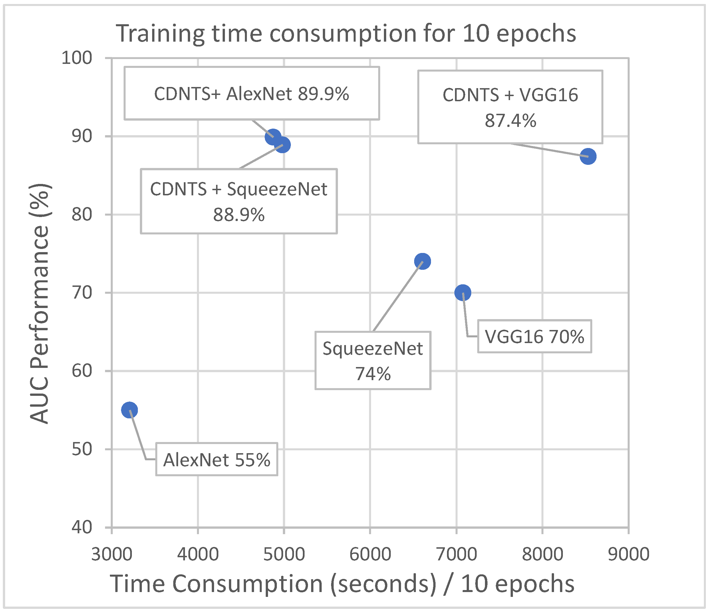
The training times of all networks used in the training and testing phase were tracked, and the durations of all networks were calculated for 10 epochs to make an accurate comparison in terms of time consumption. All training and testing stages’ time costs were calculated on a system using the GPU computing system (GeForce GTX 1080ti, Nvidia Corp., Santa Clara, CA, USA), 128 GB RAM, I7 processors, and the TensorFlow-based and Keras library.

The processing times of the train, synthetic-image test, and real-image test datasets of the CDNTS layer were measured, and values for different processes are presented in

Table 4. The CDNTS layer’s time cost list for the different datasets.

Process Name	Process Time (ms)/Each Image
Train dataset	36.7 milliseconds
Synthetic test dataset	63 milliseconds
Real test Dataset	75.9 milliseconds

. The time costs of the CDNTS layer for the train, synthetic-image test, and real-image test datasets were 36.7, 63, and 75.9 milliseconds per image, respectively. The time costs for synthetic- and real-image test datasets with the CDNTS were greater than the train dataset time cost. The train dataset consisted of segmented synthetic images, while the test dataset consisted of non-segmented images with different objects in the background. Due to this difference, the CDNTS layer detected more corners in the test dataset than the train dataset and performed more processing. For the user, the total time spent in the training process is important; in addition, the prediction time of a single image in the testing process is important. The average total time cost in the training process of 59,120 images with the CDNTS layer was 36.16 min, while the average time cost for an image in the test phase was 75.9 milliseconds per image.

The durations of the most successful networks in experiment 2 using the CDNTS layer and experiment 1 without the layer were tracked and are shown in Figure 10.

In the experiments, the CDNTS layer caused an extra 2202 s of computational time in comparison to the computations without CDNTS. This corresponds to 25% of the total training time. As the number of epoch increases, the ratio of the time cost of the CDNTS layer to the training time decreases.

5. Conclusions

This study has emphasized that classification problems with a limited size of dataset or without any dataset for training can be solved by generating synthetic data with a game engine. In addition, we have demonstrated that a dataset consisting of fully synthetic images can be used for the training process and such models can be tested on real-image classification.

In experiments 1 and 2, segmented synthetic data were trained in two different methods: DL networks and a CDNTS layer with DL networks. The models of the two experiments were tested separately with the synthetic-image dataset and the real-image dataset classifications. It was found that the inclusion of the CDNTS layer considerably improved the accuracy performance of the model. In experiment 1, the AUC value of the most successful synthetic-image test result was 74%, and the most successful real-image test result was 72%. In experiment 2, using the CDNTS network, the most successful synthetic image test result AUC value was 89.9%, and the most successful real image test result was 88.9%. The addition of the CDNTS layer to the training and test processes thus increased the accuracy performance.

The recommended method is limited to images smaller than 20 × 20 pixels. In addition, the average time cost for an image for estimating the CDNTS network is 75.9 ms. The method is suitable for applications where the time cost of 75.9 ms is ignored and the image size is larger than 20 × 20 pixels. Despite the above-mentioned limitations of our application, the present study has shown that networks can be trained with synthetic images produced by game engines using 3D models to solve real-image classification problems. Thanks to the CDNTS layer, the success of classification networks trained with synthetic data in real-image classification was increased. This study has also shown that using synthetic images is suitable for the purpose of accelerating the solving of image classification problems in which there are insufficient or no image data for training and increasing the performance of testing. At future work, it is aimed to develop a more robust classification model for night vision and thermal vision cameras. In addition, it is aimed to train artificial intelligence with synthetic data generated from just several 2D images.

References

1. Kim, J.; Gadsden, S.A.; Wilkerson, S.A. A Comprehensive Survey of Control Strategies for Autonomous Quadrotors. Can. J. Electr. Comput. Eng. 2020, 43, 3–16. [Google Scholar] [CrossRef]
2. Guan, X.; Lyu, R.; Shi, H.; Chen, J. A survey of safety separation management and collision avoidance approaches of civil UAS operating in integration national airspace system. Chin. J. Aeronaut. 2020, 33, 2851–2863. [Google Scholar] [CrossRef]
3. Chen, S.; Yin, Y.; Wang, Z.; Gui, F. Low-altitude protection technology of anti-UAVs based on multisource detection information fusion. Int. J. Adv. Robot. Syst. 2020, 17. [Google Scholar] [CrossRef]
4. Santos, I.; Castro, L.; Rodriguez-Fernandez, N.; Torrente-Patino, A.; Carballal, A. Artificial Neural Networks and Deep Learning in the Visual Arts: A review. Neural Comput. Appl. 2021, 33, 121–157. [Google Scholar] [CrossRef]
5. Gambella, C.; Ghaddar, B.; Naoum-Sawaya, J. Optimization problems for machine learning: A survey. Eur. J. Oper. Res. 2021, 290, 807–828. [Google Scholar] [CrossRef]
6. Russakovsky, O.; Deng, J.; Su, H.; Krause, J.; Satheesh, S.; Ma, S.; Huang, Z.; Karpathy, A.; Khosla, A.; Bernstein, M.; et al. ImageNet Large Scale Visual Recognition Challenge. Int. J. Comput. Vis. (IJCV) 2015, 115, 211–252. [Google Scholar] [CrossRef] [Green Version]
7. Krizhevsky, A. Learning Multiple Layers of Features from Tiny Images CIFAR-10 Dataset. 2009. Available online: https://www.cs.toronto.edu/~kriz/cifar.html (accessed on 5 April 2021).
8. Hong, S.J.; Han, Y.; Kim, S.Y.; Lee, A.Y.; Kim, G. Application of Deep-Learning Methods to Bird Detection Using Unmanned Aerial Vehicle Imagery. Sensors 2019, 19, 1651. [Google Scholar] [CrossRef] [Green Version]
9. Wang, Y.; Deng, W.; Liu, Z.; Wang, J. Deep learning-based vehicle detection with synthetic image data. IET Intell. Transp. Syst. 2019, 13, 1097–1105. [Google Scholar] [CrossRef]
10. Dogan, A.; Birant, D. Machine learning and data mining in manufacturing. Expert Syst. Appl. 2021, 166, 114060. [Google Scholar] [CrossRef]
11. Hou, L.; Chen, H.; Zhang, G.K.; Wang, X. Deep Learning-Based Applications for Safety Management in the AEC Industry: A Review. Appl. Sci. 2021, 11, 821. [Google Scholar] [CrossRef]
12. Seidaliyeva, U.; Akhmetov, D.; Ilipbayeva, L.; Matson, E.T. Real-Time and Accurate Drone Detection in a Video with a Static Background. Sensors 2020, 20, 3856. [Google Scholar] [CrossRef]
13. Du, F.; Liu, P.; Zhao, W.; Tang, X. Correlation-Guided Attention for Corner Detection Based Visual Tracking. In Proceedings of the 2020 IEEE/CVF Conference on Computer Vision and Pattern Recognition (CVPR), Seattle, WA, USA, 14–19 June 2020; pp. 6835–6844. [Google Scholar] [CrossRef]
14. Bai, Z.; Li, Y.; Chen, X.; Yi, T.; Wei, W.; Wozniak, M.; Damasevicius, R. Real-Time Video Stitching for Mine Surveillance Using a Hybrid Image Registration Method. Electronics 2020, 9, 1336. [Google Scholar] [CrossRef]
15. Duo, J.; Zhao, L. An Asynchronous Real-Time Corner Extraction and Tracking Algorithm for Event Camera. Sensors 2021, 21, 1475. [Google Scholar] [CrossRef] [PubMed]
16. Qiao, W.B.; Créput, J.C. Component-based 2-/3-dimensional nearest neighbor search based on Elias method to GPU parallel 2D/3D Euclidean Minimum Spanning Tree Problem. Appl. Soft Comput. 2021, 100, 106928. [Google Scholar] [CrossRef]
17. Keivani, O.; Sinha, K. Random projection-based auxiliary information can improve tree-based nearest neighbor search. Inf. Sci. 2021, 546, 526–542. [Google Scholar] [CrossRef]
18. Sasaki, Y. The Truth of the f-Measure. 2007. Available online: https://www.toyota-ti.ac.jp/Lab/Denshi/COIN/people/yutaka.sasaki/F-measure-YS-26Oct07.pdf (accessed on 5 April 2021).
19. Abadi, M.; Agarwal, A.; Barham, P.; Brevdo, E.; Chen, Z.; Citro, C.; Corrado, G.S.; Davis, A.; Dean, J.; Devin, M.; et al. TensorFlow: Large-Scale Machine Learning on Heterogeneous Systems. 2015. Available online: tensorflow.org (accessed on 5 April 2021).
20. Chollet, F. Keras. 2015. Available online: https://keras.io (accessed on 5 April 2021).
21. Krizhevsky, A.; Sutskever, I.; Hinton, G. ImageNet Classification with Deep Convolutional Neural Networks. In Proceedings of the NIPS’12: Proceedings of the 25th International Conference on Neural Information Processing Systems, Stateline, NV, USA, 3–8 December 2012. [Google Scholar]
22. Iandola, F.; Han, S.; Moskewicz, M.; Ashraf, K.; Dally, W.; Keutzer, K. SqueezeNet: AlexNet-level accuracy with 50× fewer parameters and <0.5 MB model size. arXiv 2016, arXiv:1602.07360v4. [Google Scholar]
23. Simonyan, K.; Zisserman, A. Very Deep Convolutional Networks for Large-Scale Image Recognition. arXiv 2015, arXiv:1409.1556. [Google Scholar]
24. Zhang, C.; Bengio, S.; Hardt, M.; Recht, B.; Vinyals, O. Understanding Deep Learning Requires Rethinking Generalization. arXiv 2017, arXiv:1611.03530v2. [Google Scholar]
25. Ros, G.; Sellart, L.; Materzynska, J.; Vazquez, D.; Lopez, A. The SYNTHIA Dataset: A Large Collection of Synthetic Images for Semantic Segmentation of Urban Scenes. In Proceedings of the 2016 IEEE Conference on Computer Vision and Pattern Recognition (CVPR), Las Vegas, NV, USA, 27–30 June 2016. [Google Scholar]
26. Zhang, Q.; Lin, G.; Zhang, Y.; Xu, G.; Wang, J. Wildland Forest Fire Smoke Detection Based on Faster R-CNN using Synthetic Smoke Images. Procedia Eng. 2018, 211, 441–446. [Google Scholar] [CrossRef]
27. Glowacz, A. Fault diagnosis of electric impact drills using thermal imaging. Measurement 2021, 171, 108815. [Google Scholar] [CrossRef]
28. Li, J.; Yan, D.; Luan, K.; Li, Z.; Liang, H. Deep Learning-Based Bird’s Nest Detection on Transmission Lines Using UAV Imagery. Appl. Sci. 2020, 10, 6147. [Google Scholar] [CrossRef]
29. Lawrence, S.; Giles, C.L.; Tsoi, A.C.; Back, A.D. Face recognition: A convolutional neural-network approach. IEEE Trans. Neural Netw. 1997, 8, 98–113. [Google Scholar] [CrossRef] [Green Version]
30. Li, Y.; Su, H.; Qi, C.R.; Fish, N.; Cohen-Or, D.; Guibas, L.J. Joint Embeddings of Shapes and Images via CNN Image Purification. ACM Trans. Graph. 2015, 34. [Google Scholar] [CrossRef]
31. Mamta, J.; Ridhima, S.; Sumindar Kaur, S.; Ravinder, K.; Divya, B.; Prashant, J. OCLU-NET for occlusal classification of 3D dental models. Mach. Vis. Appl. 2020, 3, 52. [Google Scholar] [CrossRef]
32. Lin, W.; Gao, J.; Wang, Q.; Li, X. Learning to detect anomaly events in crowd scenes from synthetic data. Neurocomputing 2021, 436, 248–259. [Google Scholar] [CrossRef]
33. Richter, S.R.; Vineet, V.; Roth, S.; Koltun, V. Playing for Data: Ground Truth from Computer Games. In Proceedings of the European Conference on Computer Vision (ECCV), Amsterdam, The Netherlands, 8–16 October 2016; Leibe, B., Matas, J., Sebe, N., Welling, M., Eds.; Springer International Publishing: Cham, Switzerland, 2016; Volume 9906, pp. 102–118. [Google Scholar]
34. Wang, Q.; Gao, J.; Lin, W.; Yuan, Y. Learning from Synthetic Data for Crowd Counting in the Wild. arXiv 2019, arXiv:1903.03303. [Google Scholar]
35. Koirala, A.; Walsh, K.B.; Wang, Z. Attempting to Estimate the Unseen—Correction for Occluded Fruit in Tree Fruit Load Estimation by Machine Vision with Deep Learning. Agronomy 2021, 11, 347. [Google Scholar] [CrossRef]
36. Morra, L.; Lamberti, F. Benchmarking unsupervised near-duplicate image detection. Expert Syst. Appl. 2019, 135, 313–326. [Google Scholar] [CrossRef] [Green Version]
37. Unity. Unity Asset Store. Available online: https://assetstore.unity.com/ (accessed on 10 February 2021).
38. Bradski, G. The OpenCV Library. Dr. Dobb’s Journal of Software Tools. 2000. Available online: https://opencv.org/ (accessed on 5 April 2021).
39. Gulamhussene, G.; Joeres, F.; Rak, M.; Pech, M.; Hansen, C. 4D MRI: Robust sorting of free breathing MRI slices for use in interventional settings. PLoS ONE 2020, 15, e0235175. [Google Scholar] [CrossRef] [PubMed]
40. Kingma, D.; Ba, J. Adam: A method for stochastic optimization. In Proceedings of the ICLR 2015, San Diego, CA, USA, 7–9 May 2015. [Google Scholar]
41. Zeiler, M.D. ADADELTA: An Adaptive Learning Rate Method. arXiv 2012, arXiv:1212.5701v1. [Google Scholar]
42. Sutskever, I.; Martens, J.; Dahl, G.; Hinton, G. On the importance of initialization and momentum in deep learning. In Proceedings of the 30th International Conference on Machine Learning, Atlanta, GA, USA, 16–21 June 2013; Volume 28, pp. 1139–1147. [Google Scholar]
43. Tieleman, T.; Hinton, G. Lecture 6.5-RMSProp. COURSERA Neural Netw. Mach. Learn. 2012, 4, 26–30. [Google Scholar]
44. Prasad, P.J.R.; Survarachakan, S.; Khan, Z.A.; Lindseth, F.; Elle, O.J.; Albregtsen, F.; Kumar, R.P. Numerical Evaluation on Parametric Choices Influencing Segmentation Results in Radiology Images—A Multi-Dataset Study. Electronics 2021, 10, 431. [Google Scholar] [CrossRef]
45. Zhao, W.; Du, S. Spectral–Spatial Feature Extraction for Hyperspectral Image Classification: A Dimension Reduction and Deep Learning Approach. IEEE Trans. Geosci. Remote Sens. 2016, 54, 4544–4554. [Google Scholar] [CrossRef]
46. Hinton, G.E.; Salakhutdinov, R.R. Reducing the Dimensionality of Data with Neural Networks. Science 2006, 313, 504–507. [Google Scholar] [CrossRef] [PubMed] [Green Version]
47. Tomasi, S.J. Good features to track. In Proceedings of the 1994 IEEE Conference on Computer Vision and Pattern Recognition, Seattle, WA, USA, 21–23 June 1994; pp. 593–600. [Google Scholar] [CrossRef]
48. Tao, Y.; Papadias, D.; Shen, Q. Chapter 26—Continuous Nearest Neighbor Search. In Proceedings of the VLDB ’02: Proceedings of the 28th International Conference on Very Large Databases, Kong, China, 20–23 August 2002; Bernstein, P.A., Ioannidis, Y.E., Ramakrishnan, R., Papadias, D., Eds.; Morgan Kaufmann: San Francisco, CA, USA, 2002; pp. 287–298. [Google Scholar] [CrossRef] [Green Version]
49. Perez, S.H.; Marinho, M.M.; Harada, K. The effects of different levels of realism on the training of CNNs with only synthetic images for the semantic segmentation of robotic instruments in a head phantom. Int. J. Comput. Assist. Radiol. Surg. 2020, 15, 1257–1265. [Google Scholar] [CrossRef]
Figure 1. Schematic representation of data preparation (left), network training (middle) and testing (right) process for experiment 1 (top) and experiment 2 (down).
Applsci 11 03863 g001
Figure 2. Green box studio designed in the unity game engine environment: (a) Virtual camera used to take a picture. (b) RW-UAV 3D model. (c) Light sources to generate realistic pictures. (d) Green-colored background, wall view. (e) Example camera view.
Applsci 11 03863 g002
Figure 3. Modern and historical city views designed in the unity game engine—virtual environments: (a) Game engine terrain of all design. (a1) Modern city design. (a2) Old city design. (bg) City views from different angles.
Applsci 11 03863 g003
Figure 4. The schematic representation related to the creation of a dataset of the RW-UAV class.
Applsci 11 03863 g004
Figure 5. Some examples of real bird and RW-UAV images. (ac) Bird images; (df) RW-UAV images.
Applsci 11 03863 g005
Figure 6. Sample output images of the CDNTS algorithm. (ad) synthetic RW-UAV and bird images samples for the training process; (a1d1) transformed shape by CDNTS layer of a–d labeled images; (e,f) synthetic RW-UAV and bird images samples for the test process; (e1,f1) transformed shape by CDNTS layer of e,f labeled images; (gj) real RW-UAV and bird images samples for the test process; (g1j1) transformed shape by CDNTS layer of gj labeled images.
Applsci 11 03863 g006
Figure 7. CDNTS layer, nearest three-point selection process schematic representation.
Applsci 11 03863 g007
Figure 8. Schematic representation of combinations of networks.
Applsci 11 03863 g008
Figure 9. Experiments 1 and 2: the precision and recall graph of the most successful networks of syntetic image test of squeezeNet with Adam optimizer (blue), real image test of SqueezeNet with Adam optimizer (orange), synthetic image test of CDNTS +AlexNet with SGD optimizer (green), real image test of CDNTS + SquezeeNet with RMSProp optimizer (red).
Applsci 11 03863 g009
Figure 10. Time cost comparison of experiments 1 and 2. Alexnet 55%, squeezenet 74%, and VGG16 70% are time cost of experiment 1. CDNTS + Alexnet 89.9%, CDNTS + squeezenet 88.9%, and CDNTS + VGG16 87.4% are time cost of experiment 2.
Applsci 11 03863 g010