Abstract
Presently, the cloud computing environment attracts many application developers to deploy their web applications on cloud data centers. Kubernetes, a well-known container orchestration for deploying web applications on cloud systems, offers an automatic scaling feature to meet clients’ ever-changing demands with the reactive approach. This paper proposes a system architecture based on Kubernetes with a proactive custom autoscaler using a deep neural network model to handle the workload during run time dynamically. The proposed system architecture is designed based on the Monitor–Analyze–Plan–Execute (MAPE) loop. The main contribution of this paper is the proactive custom autoscaler, which focuses on the analysis and planning phases. In analysis phase, Bidirectional Long Short-term Memory (Bi-LSTM) is applied to predict the number of HTTP workloads in the future. In the planning phase, a cooling-down time period is implemented to mitigate the oscillation problem. In addition, a resource removal strategy is proposed to remove a part of the resources when the workload decreases, so that the autoscaler can handle it faster when the burst of workload happens. Through experiments with two different realistic workloads, the Bi-LSTM model achieves better accuracy not only than the Long Short-Term Memory model but also than the state-of-the-art statistical auto-regression integrated moving average model in terms of short- and long-term forecasting. Moreover, it offers 530 to 600 times faster prediction speed than ARIMA models with different workloads. Furthermore, as compared to the LSTM model, the Bi-LSTM model performs better in terms of resource provision accuracy and elastic speedup. Finally, it is shown that the proposed proactive custom autoscaler outperforms the default horizontal pod autoscaler (HPA) of the Kubernetes in terms of accuracy and speed when provisioning and de-provisioning resources.
1. Introduction
With the rapid development of technology in the last decade, cloud computing has been gaining popularity in not only industry but also the academic environment [1]. A core element in cloud computing is virtualization technology, which helps cloud providers run multiple operating systems and applications on the same computing device, such as servers. Traditionally, hypervisor-based virtualization is a technique used to create virtual machines (VMs) with specific resources (e.g., CPU cores, RAM, and network bandwidth) and a guest operating system [2]. Some worldwide hypervisors include ESX, Xen, and Hyper-V. Container-based virtualization is a lightweight alternative to VMs [3], which can help decrease the start-up time and consume less resources than VMs [1]. Some well-known examples of this technology include LXC, Docker, Kubernetes, and Kata.
The main feature of cloud computing is elasticity, which allows application owners to manage unpredictable workloads, which are inherent in internet-based services [4], by provisioning or de-provisioning resources based on the demand to improve performance while reducing costs [5]. Autoscaling refers to a process that dynamically acquires and releases resources and can be categorized into two types: reactive and proactive. Reactive approaches perform scaling action by analyzing the current state of the system by setting predefined rules or thresholds. Proactive approaches analyze the historical data, predict the future, and perform scaling decisions. Selecting an appropriate autoscaling method can affect the quality of parameters, such as CPU utilization, memory, and response time, because over-provisioning leads to resource wastage and is expensive due to pay-per-use pricing, while under-provisioning degrades the system performance. Many works [6,7,8] related to hypervisor-based autoscaling solutions have been proposed, whereas the works related to container-based solutions are still on an early stage [9].
Many existing reactive autoscaling solutions use rules with thresholds that are based on infrastructure-level metrics, such as CPU utilization and memory [10,11,12]. Although these solutions are easy to implement, choosing the right values for thresholds is difficult because the workload continuously fluctuates depending on the user behavior. For proactive solutions, many works using time series data analysis have been proposed [6,7,13,14,15], whereas only a few have used machine learning algorithms for designing autoscalers [8,16,17].
Artificial intelligence technology, especially deep learning, has been implemented in many fields including computer vision, speech recognition, biomedical signal analysis, etc. [18]. It also brings a promising future to architect general autoscalers [19]. This paper aims to design a proactive autoscaling framework for Kubernetes that can provide fast and accurate scaling decisions to provision resources ahead of time. The proactive autoscaling framework uses the time series analysis method to predict the resource in the future. There are various kinds of AI approaches for time series analysis such as recurrent neural network (RNN), artificial neural network (ANN), and long short-term memory (LSTM). In contrast to other AI approaches, the bidirectional long short-term memory (Bi-LSTM) is an extension of LSTM, which is more suitable for the time series data because it can preserve the future and the past information. Thus, Bi-LSTM may have better accuracy in prediction as compared to RNN and LSTM. More technical details for how Bi-LSTM works are discussed in Section 4. The major contributions of this paper are as follows:
- First, a bidirectional long short-term memory (Bi-LSTM)-based [20] proactive autoscaling system architecture designed for Kubernetes is proposed, and it is shown that the proposed autoscaling system achieves a higher accuracy in resource estimation than the default horizontal pod autoscaler of Kubernetes.
- Second, Bi-LSTM prediction model for time-series analysis is implemented, showing that it can outperform existing proactive autoscaling time-series prediction models.
- Third, a resource removal strategy (RRS) is proposed to remove part of the resource when the workload is decreased so it can better handle a burst of workload occurring in the near future.
The results of the experiments conducted using different real trace workload datasets indicate that Bi-LSTM achieves better accuracy with not only the LSTM model but also a well-known state-of-the-art statistical method, ARIMA model, in terms of short- and long-term forecasting. In addition, the prediction speed is 530 to 600 times faster than that of the ARIMA model and almost equal compared to the LSTM model when examined with different workloads. Furthermore, compared to the LSTM model, the Bi-LSTM model performs better in terms of autoscaler metrics such as provision accuracy and elastic speedup.
The remainder of this paper is organized as follows. In Section 2, we review the recent autoscaling studies conducted using time-series analysis. In Section 3 and Section 4, the system design and concept of the proactive custom autoscaler are introduced. The prediction model is discussed in Section 5. Section 6 presents the experiment conducted for evaluating the proposed prediction model followed by the discussion in Section 7. We conclude the paper in Section 8.
2. Related Works
In this section, we review the recent studies related to autoscaling applications conducted using a time-series analysis technique in the cloud system. Time-series analysis has applications in many area such as weather forecasting, earthquake prediction, and mathematical finance. It uses previous and current observed values to predict future values [21]. In this study, it is used to predict future workload or required resources [22]. An example is the number of requests arriving at the system within one-minute intervals. Table 1 presents a review of important autoscaling methods.

Table 1.
Overview of recent works related to autoscaling methods.
Al-Dhuraibi et al. [11] presented an architecture called ELASTICDOCKER, which uses a reactive approach based on threshold-based rules to perform scaling actions. ELASTICDOCKER vertically scales both memory and virtual CPU cores resulting from the workload. The disadvantage of vertical scaling is that it has limited resources for hosting the machine capacity. To address this problem, ELASTICDOCKER performs live migration of the container when the hosting machine does not have enough resources. The experimental result showed that this approach helps reduce the cost and improve the quality of experience for end-users.
In Kubernetes (K8S), the Horizontal Pod Autoscaler (HPA) [12] is a control loop that reactively scales the number of pods based on CPU utilization, regardless of whether the workload or application is performing. It maintains an average of CPU utilization across all pods at a desired value by increasing or decreasing the number of pods, for example, .
The traditional approaches for time-series analysis and prediction include statistical methods such as autoregression (AR), moving average (MA), autoregressive moving average (ARMA), and autoregressive integrated moving average (ARIMA).
Zhang et al. [6] proposed an architecture using a reactive workload component for hybrid clouds, which classifies the incoming workload into the base workload and trespassing workload. The first workload is handled using ARIMA, while the second is handled using a public cloud.
However, the limitation of reactive approach is that it only can react to the change in workload after it actually happens. Thus, the system has to spend a certain amount of time reconfiguring to adapt to the new workload. In contrast, the proactive approach analyzes the historical data and forecasts the future resource required for the scaling action. We review some recent studies using time-series analysis for the proactive approach below.
Li and Xia [13] proposed an autoscaling platform, called the cloud resource prediction and provisioning scheme (RPPS), which can scale web applications in hybrid clouds. RPPS uses ARMA to analyze the past resource usage (CPU utilization) and forecast the future usage to provide the required resources. For the evaluation, they compared RPPS with the reactive approach of Kubernetes HPA [12] and showed that their approach achieved better results with varying workload.
Rodrigo et al. [7] proposed a cloud workload prediction module using ARIMA, which can dynamically provision VMs for serving the predicted requests. For the performance evaluation, they used real traces of HTTP web server requests from Wikimedia Foundation [26]. This model provides 91% accuracy for seasonal data; however, it is not suited for non-seasonal workload. In addition, the authors did not compare this model with any approach.
Ciptaningtyas et al. [14] also used ARIMA to predict the amount of future workload requested, as it can achieve higher accuracy for short-term forecasting. They performed evaluations using the following four ARIMA models, which had the same degree of differencing (d) as 1 and order of moving average (q) as 0 while varying the lag order value (p) from 1 to 4. The results showed that the model with lag order of 4 had the lowest prediction error for the incoming requests compared to the other models.
Messias et al. [15] proposed a prediction model using genetic algorithms (GAs) to combine many statistical methods. They used three logs extracted from real web servers to evaluate their model. The results showed that the proposed model yields the best results. However, with the NASA web server logs [27], the ARIMA model achieves the best result with the best prediction accuracy. The ARIMA model’s configuration was chosen by the auto.ari-ma() function of the R package proposed in [28] to automatically choose the value for .
The prediction model proposed in [23] used Artificial Neural Network (ANN) to forecast the task duration and resource utilization. To prepare the ANN dataset, a crawler was actualized to gather the number of files and the size of the repositories from GitHub and the task length. Then the ANN model was trained offline. The proposed model incurred less than 20% prediction error compared to a simple linear prediction model. However, as it was trained offline, this model is not suitable for real applications.
Prachimutita et al. in [8] introduced a new autoscaling framework using Artificial Neural Network (ANN) and Recurrent Neural Network (RNN) models to predict workload in the future. Then, based on the forecasted workload, they converted to the needed RAM and CPU core to keep services working under the Service Level Agreement (SLA). The performance was evaluated by using access logs from the 1998 World Cup Web site [26] for multiple-step ahead forecasting. The result showed the accuracy of ARIMA model became worse with more predicted step ahead. Furthermore, the LSTM model archived better accuracy than the MLP model.
Imdoukh et al. in [16] also proposed a machine learning-based autoscaling architecture. The resource estimator used the LSTM model and conducted an experiment on the 1998 World Cup website dataset. They compared the obtained results with those obtained by not only the ARIMA model but also the ANN model. The result showed that the proposed LSTM model has a slightly higher prediction error compared to ARIMA model in one-step forecasting, but the prediction speed is faster 530 to 600 times than the ARIMA in one-step forecasting.
Tang et al. [17] proposed a container load prediction model by using the Bi-LSTM approach, which uses the container’s past CPU utilization load to predict the future load. The accuracy of the proposed model exhibited the lowest prediction error compared to the ARIMA and LSTM models. However, the authors did not mention how to configure the parameters of the proposed model. Moreover, the paper only focuses on predicting the future load and does not apply it to solve to autoscaling problems.
Ming Yan et al. [24] proposed a hybrid elastic scaling method by combining both reactive and proactive approaches for Kubernetes. The proactive approach uses Bi-LSTM model to learn the physical host and pod resource usage history (CPU utilization, Memory usage) to predict the future workload. Then, the Bi-LSTM prediction model is combined together with the online reinforcement learning with reactive model to achieve elastic scaling decisions. Through the experiments, it is shown that it can help the system to meet microsevice SLA in edge computing environments. The Bi-LSTM model also had the smallest prediction error for the root mean square error (RMSE) metric as compared to the ARIMA, LSTM, and RNN. However, an oscillation mitigation solution has not been addressed.
Laszlo Toka et al. [25] proposed using an AI-based forecast method for proactive scaling policy. The AI-based forecast method consists of AR, Hierarchical temporal memory (HTM), and LSTM methods. Each model is used to learn and predict the rate of incoming web requests. They also proposed a backtesting plugin called HPA+ to automatically switch between methods in the AI-based model and the HPA. If the performance of AI-based model becomes poor, the HPA+ will switch to HPA and vice versa. The results show that the HPA+ can decrease the number of rejected requests significantly at the the cost of slightly more resource usage.
Most reactive approaches use rule-based model solutions. In these solutions, users have to predefine rules and set the thresholds. Although these rules are easy to implement, choosing the proper value for the thresholds is difficult because the workload continuously fluctuates depending on the user behavior. Moreover, reactive approaches can only react to workload changes after they happen and spends a certain time to reconfigure the system to adapt to the new workload. For proactive approaches, statistical methods (AR, MA, ARMA, ARIMA, etc.) are utilized to predict future workload and prepare scaling actions ahead of time. However, these techniques are relatively slow in matching dynamic workload demands. Due to the limitations of the reactive approach, we focus our work on the proactive approach only. The development of artificial intelligence, especially in deep learning, has achieved tremendous success in various fields from natural language processing, computer vision [19], and disease classification [29]. However, the use of deep learning in container autoscaling is still in its early stage. Thus, motivated by the huge success of deep learning, we propose a proactive custom autoscaler that uses the Bi-LSTM model to scale the number of pods for dynamic workload changes in Kubernetes automatically.
3. System Design
In this section, we describe our system architecture design, which is based on the monitor–analyze–plan–execute (MAPE) loop, as shown in Figure 1. The proposed architecture includes the following components:
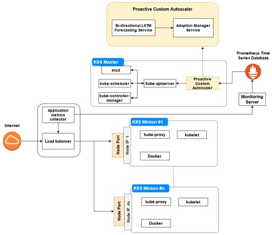
Figure 1.
System architecture.
- Load Balancer;
- Application metric collector;
- Monitor Server;
- K8S Master: etcd, kube-scheduler, kube-control-manager, kuber-apiserver, Proactive Custom Autoscaler;
- K8S Minions: kube-proxy, kubelet, Docker.
This paper mainly focuses on the proactive custom autoscaler (which includes the analysis and planning phases of the MAPE loop) described in Section 4.
3.1. Load Balancer
Load balancer provides a powerful support for containerized applications. It acts as a gateway that receives incoming TCP/HTTP requests from end-users and spreads them across multiple K8S minions. In this study, we use HAProxy [30], which is an open-source, very fast, reliable, and high-performance technology for load balancing and proxying TCP- and HTTP-based applications. The HAProxy in this paper is located outside the Kubernetes cluster. We configure the HAProxy to balance the load of all HTTP requests to all minion nodes in the Kubernetes cluster through their external NodeIP and NodePort as shown in Figure 1.
3.2. Application Metric Collector
The application metric collector is in charge of monitoring the load balancing. It collects application metrics that are applied with regard to the proposed autoscaling strategy, including the application throughput and average response time of the user’s request. Then, all information is sent to the monitoring server.
3.3. Monitoring Server
The monitoring server receives all information from the collector and sends it to a centralized time-series database. Time-series data are a series of data points indexed in order of time. Prometheus [31] is a very powerful open-source monitoring, time-series database widely used in industrial applications. It enables us to leverage the collected metrics and use them for decision-making. The collected value can be exposed by an API service and accessed by the proactive custom autoscaler.
3.4. K8S Master
In Kubernetes, each cluster comprises one master and several minion nodes. In practice, a cluster can have multiple master nodes [32] to ensure that if one master node fails, another master node will replace it and keep the system stable. The master node controls the cluster with the following four components: etcd, kube-scheduler, kube-control-manager, and kube-apiserver.
- etcd stores all the configuration data for the cluster.
- kube-scheduler searches the created and unscheduled pods to assign to nodes. It needs to consider the constraints and available resources. The nodes are then ranked and the pod is assigned to a suitable node.
- kube-control-manager watches and keeps the cluster running in the desired state. For instance, an application is running with five pods, after a period time, one pods is down or missing, so the kube-control-manager creates a new replica for that missing pod.
- kube-apiserver validates and manages the components of the cluster, including pods, services, and replication controllers. Each change in the cluster’s state has to pass through kube-apiserver, which manages the minion nodes through the kubelet.
3.5. K8S Minion
A minion hosts the pods and runs them following the master’s instructions.
- kubelet is an agent that runs on each node of the cluster. It is instructed by kube-apiserver of Master and keep the containers healthy and alive.
- kube-proxy controls network rules on the nodes. These rules allow the network communication to the pods from internal or external network of your cluster.
- Docker: Kubernetes is one the most common specialized orchestration platforms for a containerized application. In this study, we select Docker [33], which is a lightweight, portable, self-sufficient, and the most popular container engine for Kubernetes.
- NodeIP is an external IP address of a minion node. This IP address is accessible from the internet.
- NodePort is an open port on every minion node of the cluster and exposes the application across each of minion nodes. The NodePort’s value has predefined range between 30,000 and 32,767.
4. Proactive Custom Autoscaler
As mentioned earlier, the system architecture is based on MAPE loop, and our main contributions are Bi-LSTM forecasting service (as the analysis phase) and the adaptation manager service (as the planning phase), which are regarded as core of autoscaler. Figure 2 shows the architecture of the autoscaler with four main phases. Next, we describe each phase in this autoscaler in detail.
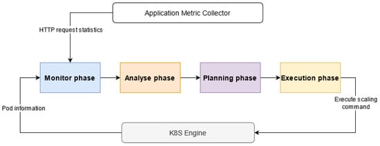
Figure 2.
Autoscaler architecture.
4.1. Monitor Phase
In this phase, the monitoring server, described in Section 3, continuously receives different types of data for analysis and planning phases to determine appropriate scaling actions. In this paper, the different types of data are collected from two sources: (1) the networking data of the load balancer, such as number of HTTP requests per second through the application metric collector, and (2) pod information of all running nodes such as the number of pod replicas, which are retrieved from the master node (using kube-apiserver).
After collecting the data, the monitoring server begins to aggregate and sends it to Prometheus time-series database. By adding a time series database, we can maintain all collected data as historical record and use it to train the prediction model to improve model’s prediction accuracy.
4.2. Analysis Phase—Bi-LSTM Forecasting Service
In the analysis phase, the Bi-LSTM forecasting service period obtains the latest collected metric data with window size w through Prometheus’s restful API. The trained model then uses these latest data to predict the next data in sequence . In our implementation, the Bi-LSTM neural network model was used to predict workload of HTTP requests in the future. Thus, we will discuss the Bi-LSTM neural network model in more detail.
First, we discuss the standard (known as Forward or Uni-) Long Short-Term Memory (LSTM). LSTM is a member of the deep RNN family, which is used in many fields, including sentiment analysis, speech recognition, and time-series analysis. It is a modified version of the RNN architecture, and was first introduced by Hochreiter and Schmihuber [34] in 1996 and popularized by many studies thereafter. Unlike the feed-forward neural network, RNNs take the current and previous time-step output data as input to build the network [35]. There were networks with loops in them, which allow the history data to be maintained. However, traditional RNNs incur long-term dependencies due to the gradient vanishing problem. In RNNs, the gradient expands exponentially over time [36]. To address this problem, LSTM, which is a special type of RNN, has been proposed [37]. However, LSTM can only handle information in one direction, which is a limitation because it ignores the continuous data changes. Therefore, LSTM can only capture partial information.
The regular RNN or LSTM traverses input sequence with forward direction of the original time series. The Bi-LSTM [20] are an extension of the LSTM models with two LSTMs applied to the input data. The first LSTM is trained on the input sequence with its original direction (forward). The second LSTM is fed with the reverse form of the input sequence (backward). This architecture of Bi-LSTM is two LSTM networks stacked on top of each other. It bidirectionally runs the input from two directions, the first one from past to future, the second from future to past. The difference from forward LSTM is that running backward helps preserve information from the future. By combining two hidden states, one can preserve information from the past and the future. Applying the LSTM twice leads to improved learning long-term dependencies and thus consequently will improve the accuracy of the model [38].
The Bi-LSTM processes data in both directions with two separate hidden LSTM layers to get more data. The Bi-LSTM equations are expressed as (1)–(3) below:
where and , and , and and are different weight matrices. f denotes the activation functions, for example, Tanh sigmoid or logistic sigmoid; and , , and are the forward, backward, and output layer biases, respectively.
Given an input sequence , a Bi-LSTM computes the forward hidden sequence, , the backward hidden sequence, , and the output sequence, , by iterating the forward layer from to T and the backward layer from to 1 and then updating the output layer.
For the t-th time step, both parallel hidden layers in both forward and backward directions process as input. The hidden states and are the output results of two hidden layers in both forward and backward directions at time step t, respectively. Then the output value depends on the sum of the hidden states and , as described in Equation (3).
4.3. Planning Phase—Adaption Manager Service
In this phase, The Adaption Manager Service calculates the number of pods required for provisioning or de-provisioning based on the predicted workload of HTTP requests from the previous step. It is designed to scale in and scale out pods to meet future workload.
Algorithm 1 explains our scaling strategy after the predictor provides the amount of HTTP requests in the next interval, . Because of oscillation problem, the scaler performs opposite actions frequently within a short period [9], which wastes resources and costs. To address this problem, we set the cooling down time (CDT) to 60 s (1 min) after each scaling decision, which is fine-grained compared to the container’s scenery. We denote as the maximum workload that a pod can process in a minute and as the number of minimum pods should be maintained and the system cannot scale down the number of pods that lower than this value. During the system’s operation, for each minute, we calculate the number of pods required, , in the next time step and compare it with that of the current pods, . If the required pods exceed the current pods , the scaling out command is triggered and the scaler increases the number of pods to meet the resource demand in the near future. Otherwise, if the number of required pods is lower than the number of current pods, the scaler removes an amount of surplus pods, , which follows the resource removal strategy (RRS), to stabilize the system while handling it faster if a burst of workload occurs in the the next interval. First, we use the max function to the choose higher value between the and value for updating the value. This must be done because the system cannot scale down to a lower number than value. Second, the number of surplus pods, which follows the RRS, is calculated as per Equation (4):
| Algorithm 1: Adaption Manager Service algorithm. |
 |
Then, we update the value of by using the current pods’ value minus the surplus pods’ value achieved in previous step. By doing this, we only need to remove a part of surplus resources (pods), not all of them. Finally, we execute the scale in command with the final updated value. Using the RRS strategy not only helpss the system to stabilize with the low workload but also to adapt faster with the burst of workload because it spends less time to create and update the number of pods. In our experiments, we set RRS to 0.60 (60%) and to 10.
4.4. Execution Phase
In this last phase of MAPE loop, the Kubernetes engine (kube-apiserver) receives command from Adaption manager service of planning phase and changes number of pod replicas.
5. Bi-LSTM Prediction Model
The proposed Bi-LSTM prediction model is discussed in this section.
5.1. Neural Network Architecture
The proposed Bi-LSTM model is shown in Figure 3, which has two layers that move forward and backward. Each hidden layer contains an input layer with 10 neural cells for the last 10 time steps, with 30 hidden units for each neural cell. The final outputs of the hidden layers in both forward and backward directions are concatenated and be used as input to the Dense. The Dense is a fully connected layer, which means each neuron in the Dense receives input from all neurons of previous layer. The output shape of the Dense will be affected by the number of neuron specified in it. In this study, the Dense is used to output predictions. Because the model is non-linear regression model, we use the ReLU activation function in the hidden layer.
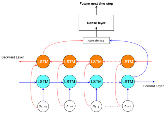
Figure 3.
Proposed bidirectional LSTM network architecture.
5.2. Single-Step and Multi-Step Predictions
In time-series analysis, a prediction problem that requires prediction of the next time step is called single-step prediction, while the one that requires prediction of more than one step is called multi-step prediction.
6. Experiment and Evaluation
In this section, we evaluate the proposed system design presented in Section 3. First, the proposed Bi-LSTM model is evaluated and its accuracy and prediction speed are compared with those of the forward LSTM in [16] and ARIMA in [14,39] by using different datasets. Subsequently, a complete proposed system in Section 3 is simulated and evaluated in a real environment to see the performance in terms of provision accuracy and elastic speedup.
6.1. Datasets
We evaluate our proposed model using two real web server logs: two months of NASA web servers [27] and three months of FIFA World Cup 98 web servers [40].
6.1.1. NASA Dataset
The NASA logs were collected by the NASA Kennedy Space Center WWW server in Florida for two months, and can be classified into two sub-logs [27]. The first log contains all HTTP requests made from 00:00:00 1 July 1995, to 23:59:59 31 July 1995 (total 31 days). The second log contains requests made from 00:00:00 1 August 1995, to 23:59:59 31 August 1995. These two logs contain 3,461,612 requests in total. Because of Hurricane Erin, the server was shut down, so there were no logs between 1 August 1995 14:52:01 and 3 August 1995 04:36:13. This dataset has been used in [15,41,42] and others to evaluate the autoscalers.
We preprocessed the original dataset by aggregating all logs occurring in the same minute into one accumulative record. Thus, the dataset now represents the total workload for each minute. The preprocessed dataset is shown in Figure 4, which indicates a repetitive data pattern within a certain period.
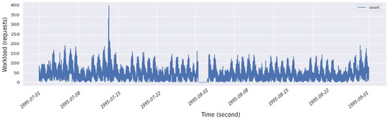
Figure 4.
NASA dataset.
6.1.2. FIFA Worldcup Dataset
The FIFA World Cup dataset contains 1,352,804,107 requests, logged from 30 April 1998 to 26 July 1998. This dataset has been extensively used [15,16,43,44] to study autoscalers. Similar to the NASA dataset, this dataset was also preprocessed by aggregating all logs that occurred within the same minute into one accumulative record, as shown in Figure 5.
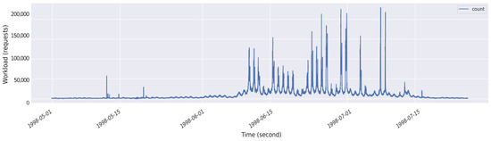
Figure 5.
FIFA dataset.
The distribution of this dataset is more complicated than that of NASA. This is because the FIFA World Cup dataset has a high degree of variation in its value; moreover, it does not have a pattern like NASA and has peaks that are difficult to predict.
6.2. Experiment Explanation
As described in the beginning of the section, we conduct two experiments to evaluate the custom autoscaler. In the first experiment, we use both NASA and FIFA World Cup datasets for training and evaluating the prediction models. We split each dataset into 70% for the training set and 30% for the testing set. The Bi-LSTM prediction model explained in Section 5 is compared with the forward LSTM and ARIMA prediction models. The configuration of each compared model differs based on different datasets. The configuration of Bi-LSTM model is described in Table 2. The Bi-LSTM and LSTM models were implemented using Keras library from the TensorFlow software library [45]. We also used StatsModel library [46] to implement ARIMA models. All prediction models were implemented using Python programming language and trained on tensor processing unit (TPU) from Google Colab [47]. The implementations and evaluations of these prediction models follow the tutorials at [48,49].
Table 2.
Bi-LSTM model configuration.
The following two types of prediction models were used in the experiments: a one-step (1 step) prediction model, which uses the last 10 min workload to predict the total workload in the next minute, and a five-step (5 steps) prediction model, which uses a multi-step prediction strategy to predict the total workload in the next 5 min by using the last 10 min workload. Both forward LSTM and Bi-LSTM in this experiment use the mean square error (MSE) as a loss function for the training process to avoid over-fitting and early stopping, and to stop the training process when the validation loss does not decrease any further.
In the second experiment, we simulated the environment to see the performance in terms of resource provision accuracy and elastic speedup. The simulation was implemented using the Python programming language and running on Google Colab environment. We retrieved a subset from the FIFA World Cup 98 database and input them into the proactive custom autoscaler, which then uses Algorithm 1 to calculate the number of pods required to maintain the stability of the system. In this simulation experiment, we assumed that one pod can contain one Docker container. We also assumed that one pod can process 500 HTTP requests for a minute, and the workload was balanced between deployed pods.
For further experiments, we built the proposed architecture in Section 3 in a real environment, and compared the proposed proactive custom autoscaler with the default autoscaler of Kubernetes HPA in terms of responsiveness. The Kubernetes cluster is implemented with one master node and three minion nodes. Each node on the cluster runs on a virtual machine. Table 3 shows the system configurations. The master node had 12GB of Random-access memory (RAM) and 8 CPU cores, while each minion had 4GB of RAM and 4 CPU cores. We also set up one pod that could have only one container. The proactive custom autoscaler was executed on the master node. We used Apache JMeter [50], which is an open-source load testing tool for web application to generate the HTTP requests to the HAProxy. The HAProxy continues receiving HTTP requests from the JMeter and forwarding them to the minion nodes via their external NodeIPs and NodePorts for processing. The NodePort’s value is set to 31000. The minions have simple web applications deployed on them to process the user requests. The web application returns a simple json string as shown in Figure 6. The application metric collector collects information about the application throughput and sends it to the monitoring server, which starts aggregating the collected data and stores it in the Prometheus time-series database [51]. The proactive custom autoscaler retrieves the workload for the last 10 minutes through Prometheus’s API, starts predicting the workload for the next minute, and calculates the number of pods required by using the proposed Algorithm 1. The execution command in the algorithm communicates with kube-apiserver to create (or remove) the number of pods. For the HPA, we set the target CPU utilization threshold to 70% and the number of replicas between 12 and 30.
Table 3.
System configurations.
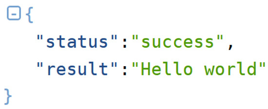
Figure 6.
The returned result of simple HTTP server.
6.2.1. Configuration of Models Compared for the NASA Dataset
For the NASA dataset, we compared our model with the ARIMA model. The parameters of ARIMA are chosen by the auto.ari-ma() function, as suggested in [15].
6.2.2. Configuration of Models Compared for FIFA Worldcup 98 Dataset
For the FIFA dataset, the compared models were forward LSTM and ARIMA.
The architecture of forward LSTM comprised 10 neural cells for the input layer, 30 LSTM units for one hidden layer, and 1 neural cell for the output layer, as suggested in [16]; the early stopping was set to 2. We also normalized the FIFA Worldcup dataset to a range within [−1, 1] by using Equation (5).
The ARIMA model is configured with a lag order (p) of 4, degree differencing (d) set as 1, and order of moving average (q) set as 0, as suggested in [14].
6.3. Evaluation Metrics
To evaluate the accuracy of the proposed model, we used four metrics as shown in Equations (6)–(9), respectively. These metrics are used to compare the prediction accuracies of the models. We define as the actual value, as the forecast value, and as the mean value of . In addition, we also compare the average prediction speed of 30 tries that each model takes for prediction.
The mean square error (MSE) in Equation (6) calculates the average squared difference between the forecast and the observed values. The root mean square error (RMSE), expressed as Equation (7), represents the square root of two of the differences between the forecast and observed values. The mean absolute error (MAE), expressed as Equation (8), represents the average over the test sample of the absolute differences between the prediction and actual observation, where all individual differences have equal weights. The metrics MSE, RMSE, MAE are used to evaluate the prediction error of the models, where a smaller value indicates a higher prediction accuracy and vice versa. The coefficient of determination, denoted as , is shown in Equation (9) as a goodness-of-fit measure for linear regression models. It is the square of the coefficients of multiple correlations between the observed outcomes and the observed predictor values. The higher the , the better the model fits the data.
Furthermore, to evaluate the provision accuracy and elastic speedup of the autoscaler, we used system-oriented elasticity metrics endorsed by the Research Group of the Standard Performance Evaluation Corporation (SPEC) [52], as shown in Equations (10)–(14). These metrics have also been used by other researchers [16,53]. We denote and as the required resource and provide resources at time , respectively. is the time interval between the last and the current changes in the resource either in the required r or provided p.
For resource provisioning accuracy, the under-provisioning metric defines the number of missing pods that are required to meet the service-level objective (SLOs) normalized by the measured time. The over-provisioning metrics identify the number of surplus pods provided by the autoscaler. The range of and is from 0 to infinity ∞, where 0 is the best value. and correspond to the duration of prediction when the system is under-provisioned and over-provisioned, respectively. The range of and are from 0 to 100, and the best value is 0 when there is no under- or over-provisioning during measurement time. Finally, the elastic speedup, , is the autoscaling gain compared to the no autoscaling case, where are cases when using autoscaling and are otherwise. If the has a value greater than 1, the proposed auto-scaler has an autoscaling gain over no auto-scaler and vice versa.
6.4. Experiment Results
6.4.1. NASA Dataset
The Bi-LSTM model shown in Table 4 achieves the smaller prediction error values on MSE, RMSE, MAE metrics compared to the ARIMA model in both single-step (one-step) and multi-step (five-step) predictions. This means the Bi-LSTM has better prediction accuracy than the ARIMA model. Furthermore, the values of the Bi-LSTM model in both one-step and five-step predictions are higher than those of the ARIMA model, which shows that the Bi-LSTM can fit the data better than ARIMA. Finally, Bi-LSTM not only improves in terms of all metrics but also has a faster prediction speed by 530 and 55 times following one-step and five-step predictions, respectively, compared to the statistical method ARIMA.
Table 4.
Experiment result on NASA dataset.
Figure 7 and Figure 8 present the result of the predicted value versus the actual value. The performance of ARIMA model appears to be similar to the Bi-LSTM model. Then, we take a closer look by zooming in to the results. Figure 9 shows the absolute error of models for the first 100 minutes of the testing set. We can observe that the ARIMA model usually has higher absolute error values than the Bi-LSTM model. Therefore, the Bi-LSTM model performs better not only in terms of prediction accuracy but also prediction speed compare to the ARIMA model.
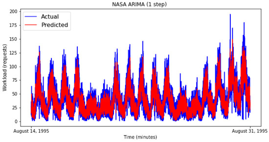
Figure 7.
ARIMA with one-step prediction on the testing set.
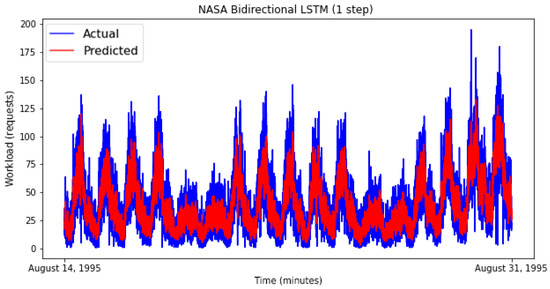
Figure 8.
Bi-LSTM with one-step prediction on the testing set.
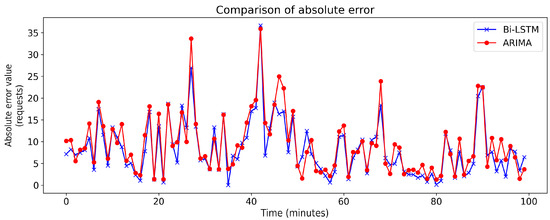
Figure 9.
Comparison of absolute error for the first 100 minutes of NASA testing set.
6.4.2. FIFA Worldcup 98 Dataset
Table 5 shows the experimental results obtained for the FIFA Worldcup 98 dataset. The Bi-LSTM model outperforms all other models, including the statistical method ARIMA and feed-forward LSTM models, because it has the smallest prediction error values on MSE, RMSE MAE metrics in both one-step and five-step predictions. In five-step prediction, RMSE of the Bi-LSTM is 1.31 and 1.25 times smaller than those of ARIMA and forward LSTM, respectively, which indicates better accuracy. The Bi-LSTM not only has a better prediction accuracy but also has a prediction speed 600 times faster than that of the well-known short-term statistical ARIMA in one-step predictions. Although the prediction speed of Bi-LSTM is higher than that of the feed-forward LSTM, the speed is measured in milliseconds, which is too minor to consider.
Table 5.
Experiment result on FIFA Worldcup 98 dataset.
Figure 10, Figure 11 and Figure 12 indicate the results obtained for the testing set. As the difference between these results is negligible, we focus on a small part of this dataset to obtain a better observation. We use the results obtained from 1 July 1998 20:31:00 to 2 July 1998 05:00:00, as shown in Figure 13, Figure 14 and Figure 15. Figure 13 shows that the ARIMA model tends to over-predict and under-predict most of the time. While the LSTM model shown in Figure 14 tends to over-predict through the time, the predicted values provided by Bi-LSTM model in Figure 15 nearly match the actual values. Thus, the Bi-LSTM model has better prediction accuracy than ARIMA and the forward LSTM model.
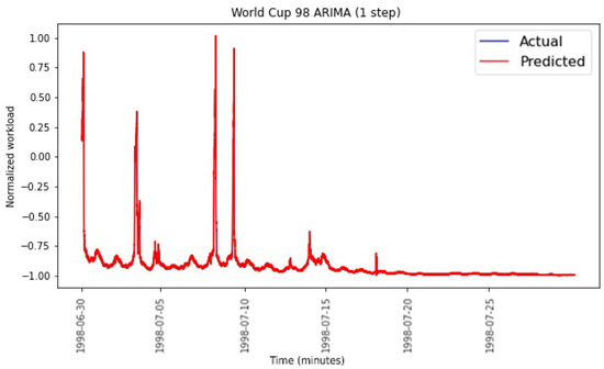
Figure 10.
ARIMA with one-step prediction on the testing set.
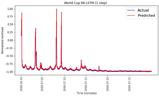
Figure 11.
Forward LSTM with one-step prediction on the testing set.
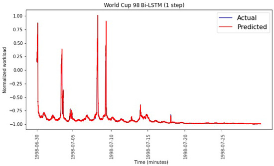
Figure 12.
Bi-LSTM with one-step prediction on the testing set.
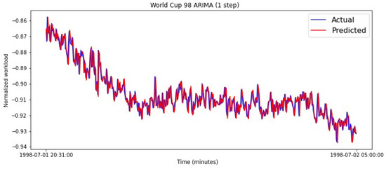
Figure 13.
ARIMA with one-step prediction on the testing set (from 1 July 1998 20:31:00 to 2 July 1998 05:00:00).
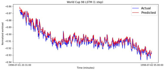
Figure 14.
Forward LSTM with one-step prediction on the testing set (from 1 July 1998 20:31:00 to 2 July 1998 05:00:00).
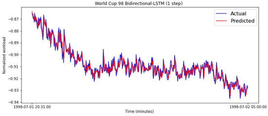
Figure 15.
Bi-LSTM with one-step prediction on the testing set (from 1 July 1998 20:31:00 to 2 July 1998 05:00:00).
6.4.3. Evaluation of Autoscaler
Because the ARIMA model exhibits a poor prediction speed, it is not suitable for real-time autoscaling systems and thus is not considered in this experiment. For this experiment, we took a testing subset of the NASA dataset from 7 July 1998 09:51:00 to 1 July 1998 16:31:00. Figure 16 and Figure 17 show the number of pods produced by the LSTM and Bi-LSTM autoscalers for the one-step prediction. A comparison of both autoscalers is shown in Table 6, where Bi-LSTM achieves better performance in and in one-step and five-step predictions. These results show that the proposed Bi-LSTM autoscaler tends not to have over-provision, and when it does, it occurs for a shorter time as compared to LSTM. In contrast, the LSTM autoscaler achieves better performance in (both one-step and five-step predictions), and the of both autoscalers are almost equal in the one-step prediction. It is shown that LSTM tends not to have under-provision as compared to Bi-LSTM. Finally, the Bi-LSTM autoscaler outperforms the LSTM autoscaler in elasticity speedup in both one-step and five-step predictions, which indicates that Bi-LSTM has a higher autoscaling gain over LSTM.
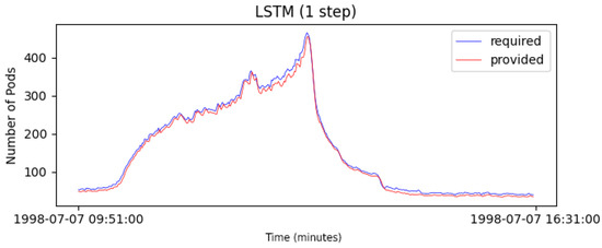
Figure 16.
Number of pods produced by the LSTM auto-scaler.
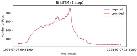
Figure 17.
Number of pods produced by the Bi-LSTM auto-scaler.
Table 6.
Evaluation of auto-scaler.
Figure 18 shows the changes in the number of pods of the proposed proactive custom autoscaler (PCA) and the HPA for the given workload in a real environment. By default, every 15 seconds, also known as the sync period, the HPA will compare the collected metric values against their predefined thresholds. In this experiment, the metric for the HPA is CPU usage, and its threshold is 70%. Once the average CPU usage exceeds the predefined threshold, the HPA will calculate and increase the number of pods in the cluster. There will be a delay time for creating new pods and assigning them to the nodes, which is the common drawback of the reactive approach. It only reacts to workload changes after it happens and spends a certain time reconfiguring the system to adapt to the new workload. In addition, the default value for down scaling is 5 minutes. This means that the HPA will keep monitoring the average CPU usage, and if its value is below the threshold for 5 min, HPA will start scaling down. This mechanism of HPA is called cooldown/delay [12]. It is shown in Figure 18 that the scaling down actions happen quite late, around the 20th and 83rd min, which leads to a waste of resources due to a slow response to traffic demand change. In contrast, the proactive custom autoscaler (PCA) has better performance in accuracy and speed than HPA because PCA can predict the trend of workload and perform the scaling up/down actions more accurately and ahead of time. Moreover, when the workload decreases, the PCA was found to remove a part of pod replicas, thus making it efficient when handling a burst of workload in the near future.
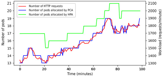
Figure 18.
Evaluation of proposed auto-scaler in the real environment.
7. Discussion
Through the experiments, it was observed that the Bi-LSTM is more suitable for estimating the resources in the Kubernetes cluster than statistical ARIMA and the feed-forward LSTM. More specifically, the Bi-LSTM prediction model was compared with the ARIMA prediction model in Table 4. It is shown that the Bi-LSTM has a higher prediction accuracy as compared to ARIMA. It reduces prediction error by 3.28% in one-step prediction and 6.64% in five-step prediction on RMSE metric. The prediction speed is 530 and 55 times faster than ARIMA in one-step and five-step predictions.
In addition, the Bi-LSTM is compared with LSTM in Table 5 and Table 6. It is shown that the Bi-LSTM achieves higher prediction accuracy than LSTM. It reduces prediction error by 7.79% in one-step prediction and 20% in five-step prediction on RMSE metric. It also achieves comparable prediction speed to LSTM in one-step and five-step predictions. It is observed from Table 6 that Bi-LSTM has more errors in prediction when decreasing resources, and has less error in prediction when increasing the resources as compared to LSTM. Obviously, Bi-LSTM outperforms LSTM in the overall prediction accuracy as shown in Table 5. It can also be observed from the elastic speedup results in Table 6 that the Bi-LSTM autoscaler has a higher autoscaling gain than the LSTM autoscaler in both one-step and five-step predictions.
The proposed architecture in this work is based on the existing components of the Kubernetes. However, this architecture can also be implemented in other container-based platforms, such as using Docker Swarm for orchestration and other container engines like OpenVZ, LXC. This is because the Bi-LSTM forecasting service and the Adaption manager service can analyze and process the monitored data (networking data, and pods or containers information) to calculate appropriate scaling decisions and are independent not only from the container virtualization technology but also from the cloud providers. Furthermore, we can change and update the Bi-LSTM forecasting service to learn and predict more hardware metrics such as CPU utilization and memory usage for more accurate scaling decisions.
8. Conclusions
The concept of microservices and cloud services provides a new method of application development and service operation. Autoscaling is one the most essential mechanisms that autonomic provisioning or de-provisioning resources based on the demand to improve performance while reducing costs in cloud environment. This paper proposes a system architecture based on the Kubernetes orchestration system with a proactive custom autoscaler using a deep neural network model to calculate and provide resources ahead of time. The proposed autoscaler focuses on the analysis and planning phases of the MAPE loop. In the analysis phase, we used a prediction model based on Bi-LSTM, which learns from the historical time-series request rate data to predict the future workload. The proposed model was evaluated through a simulation and the real workload trace from NASA [27] and FIFA [40]. The planning phase implements cooling down time (CDT) to prevent the oscillation mitigation problem, and when the workload decreases, the scaler uses the resource removal strategy (RRS) to simply remove an amount of surplus pods to maintain the system stability while handling it faster if a burst of workload occurs in the next interval. The results of an experiment conducted with different datasets indicate that the proposed prediction model achieves better accuracy not only than the LSTM model but also than the state-of-the-art statistical ARIMA model in terms of short- and long-term forecasting. The prediction speed is 530 to 600 times faster than that of the ARIMA model and almost equal compared to the LSTM model when examined with different workloads. Compared to the LSTM model, the Bi-LSTM model performs better in terms of autoscaler metrics for resource provision accuracy and elastic speedup. Moreover, when the workload decreases, the architecture was found to remove a part of pod replicas, thus making it efficient when handling burst of workload in the near future. Finally, the proposed system design shows better performance in accuracy and speed than the default horizontal pod autoscaler (HPA) of the Kubernetes when provisioning and de-provisioning resources.
In this paper, we only focus on the horizontal autoscaling that adds and remove pods. In the future, we plan to extend our work to vertical autoscaling that adds or removes resources (e.g., CPU, RAM) of deployed pods and hybrid autoscaling by combining both horizontal and vertical scalings.
Author Contributions
N.-M.D.-Q. proposed the idea, performed the analysis, and wrote the manuscript. M.Y. provided the guidance for data analysis and paper writing. All authors have read and agreed to the published version of the manuscript.
Funding
This research was funded by the MSIT (Ministry of Science and ICT), Korea, under the ITRC (Information Technology Research Center) support program (IITP-2021-2017-0-01633) supervised by the IITP (Institute for Information and Communications Technology Planning & Evaluation).
Institutional Review Board Statement
Not applicable.
Informed Consent Statement
Not applicable.
Data Availability Statement
Not applicable.
Conflicts of Interest
The authors declare no conflict of interest.
References
- Al-Dhuraibi, Y.; Paraiso, F.; Djarallah, N.; Merle, P. Elasticity in Cloud Computing: State of the Art and Research Challenges. IEEE Trans. Serv. Comput. 2018, 11, 430–447. [Google Scholar] [CrossRef]
- Varghese, B.; Buyya, R. Next generation cloud computing: New trends and research directions. Future Gener. Comput. Syst. 2018, 79, 849–861. [Google Scholar] [CrossRef]
- Pahl, C.; Brogi, A.; Soldani, J.; Jamshidi, P. Cloud Container Technologies: A State-of-the-Art Review. IEEE Trans. Cloud Comput. 2017. [Google Scholar] [CrossRef]
- Fernandez, H.; Pierre, G.; Kielmann, T. Autoscaling Web Applications in Heterogeneous Cloud Infrastructures. In Proceedings of the 2014 IEEE International Conference on Cloud Engineering, Boston, MA, USA, 11–14 March 2014; pp. 195–204. [Google Scholar]
- Cruz Coulson, N.; Sotiriadis, S.; Bessis, N. Adaptive Microservice Scaling for Elastic Applications. IEEE Internet Things J. 2020, 7, 4195–4202. [Google Scholar] [CrossRef]
- Zhang, H.; Jiang, G.; Yoshihira, K.; Chen, H.; Saxena, A. Intelligent Workload Factoring for a Hybrid Cloud Computing Model. In Proceedings of the 2009 Congress on Services—I, Los Angeles, CA, USA, 6–10 July 2009; pp. 701–708. [Google Scholar]
- Calheiros, R.N.; Masoumi, E.; Ranjan, R.; Buyya, R. Workload Prediction Using ARIMA Model and Its Impact on Cloud Applications’ QoS. IEEE Trans. Cloud Comput. 2015, 3, 449–458. [Google Scholar] [CrossRef]
- Prachitmutita, I.; Aittinonmongkol, W.; Pojjanasuksakul, N.; Supattatham, M.; Padungweang, P. Auto-scaling microservices on IaaS under SLA with cost-effective framework. In Proceedings of the 2018 Tenth International Conference on Advanced Computational Intelligence (ICACI), Xiamen, China, 29–31 March 2018; pp. 583–588. [Google Scholar]
- Qu, C.; Calheiros, R.N.; Buyya, R. Auto-Scaling Web Applications in Clouds: A Taxonomy and Survey. ACM Comput. Surv. 2018, 51. [Google Scholar] [CrossRef]
- Taherizadeh, S.; Stankovski, V. Dynamic Multi-level Auto-scaling Rules for Containerized Applications. Comput. J. 2018, 62, 174–197. [Google Scholar] [CrossRef]
- Al-Dhuraibi, Y.; Paraiso, F.; Djarallah, N.; Merle, P. Autonomic Vertical Elasticity of Docker Containers with ELASTICDOCKER. In Proceedings of the 2017 IEEE 10th International Conference on Cloud Computing (CLOUD), Honolulu, HI, USA, 25–30 June 2017; pp. 472–479. [Google Scholar]
- Horizontal Pod Autoscaler. Available online: https://kubernetes.io/docs/tasks/run-application/horizontal-pod-autoscale (accessed on 1 August 2020).
- Fang, W.; Lu, Z.; Wu, J.; Cao, Z. RPPS: A Novel Resource Prediction and Provisioning Scheme in Cloud Data Center. In Proceedings of the 2012 IEEE Ninth International Conference on Services Computing, Honolulu, HI, USA, 24–29 June 2012; pp. 609–616. [Google Scholar]
- Ciptaningtyas, H.T.; Santoso, B.J.; Razi, M.F. Resource elasticity controller for Docker-based web applications. In Proceedings of the 2017 11th International Conference on Information Communication Technology and System (ICTS), Surabaya, Indonesia, 31 October 2017; pp. 193–196. [Google Scholar]
- Messias, V.R.; Estrella, J.C.; Ehlers, R.; Santana, M.J.; Santana, R.C.; Reiff-Marganiec, S. Combining time series prediction models using genetic algorithm to autoscaling Web applications hosted in the cloud infrastructure. Neural Comput. Appl. 2016, 27, 2383–2406. [Google Scholar] [CrossRef]
- Imdoukh, M.; Ahmad, I.; Alfailakawi, M.G. Machine learning-based auto-scaling for containerized applications. Neural Comput. Appl. 2019, 32, 9745–9760. [Google Scholar] [CrossRef]
- Tang, X.; Liu, Q.; Dong, Y.; Han, J.; Zhang, Z. Fisher: An Efficient Container Load Prediction Model with Deep Neural Network in Clouds. In Proceedings of the 2018 IEEE Intl Conf on Parallel Distributed Processing with Applications, Ubiquitous Computing Communications, Big Data Cloud Computing, Social Computing Networking, Sustainable Computing Communications (ISPA/IUCC/BDCloud/SocialCom/SustainCom), Melbourne, Australia, 11–13 December 2018; pp. 199–206. [Google Scholar]
- Paszkiel, S. Using Neural Networks for Classification of the Changes in the EEG Signal Based on Facial Expressions. In Analysis and Classification of EEG Signals for Brain–Computer Interfaces; Springer: New York, NY, USA, 2020; pp. 41–69. [Google Scholar]
- Pouyanfar, S.; Sadiq, S.; Yan, Y.; Tian, H.; Tao, Y.; Reyes, M.P.; Shyu, M.L.; Chen, S.C.; Iyengar, S.S. A Survey on Deep Learning: Algorithms, Techniques, and Applications. ACM Comput. Surv. 2018, 51. [Google Scholar] [CrossRef]
- Schuster, M.; Paliwal, K.K. Bidirectional recurrent neural networks. IEEE Trans. Signal Process. 1997, 45, 2673–2681. [Google Scholar] [CrossRef]
- Time Series Analysis. Available online: https://en.wikipedia.org/wiki/Time_series (accessed on 3 March 2021).
- Singh, P.; Gupta, P.; Jyoti, K.; Nayyar, A. Research on Auto-Scaling of Web Applications in Cloud: Survey, Trends and Future Directions. Scalable Comput. Pract. Exp. 2019, 20, 399–432. [Google Scholar] [CrossRef]
- Borkowski, M.; Schulte, S.; Hochreiner, C. Predicting Cloud Resource Utilization. In Proceedings of the 2016 IEEE/ACM 9th International Conference on Utility and Cloud Computing (UCC), Shanghai, China, 6–9 December 2016; pp. 37–42. [Google Scholar]
- Yan, M.; Liang, X.; Lu, Z.; Wu, J.; Zhang, W. HANSEL: Adaptive horizontal scaling of microservices using Bi-LSTM. Appl. Soft Comput. 2021, 105, 107216. [Google Scholar] [CrossRef]
- Toka, L.; Dobreff, G.; Fodor, B.; Sonkoly, B. Adaptive AI-based auto-scaling for Kubernetes. In Proceedings of the 2020 20th IEEE/ACM International Symposium on Cluster, Cloud and Internet Computing (CCGRID), Melbourne, Australia, 11–14 May 2020; pp. 599–608. [Google Scholar]
- Page View Statistics for Wikimedia Projects. Available online: http://dumps.wikimedia.org/other/pagecounts-raw (accessed on 1 August 2020).
- Two Month’s Worth of All HTTP Requests to the NASA Kennedy Space Center. Available online: fttp://ita.ee.lbl.gov/html/contrib/NASA-HTTP.html (accessed on 1 August 2020).
- Hyndman, R.; Khandakar, Y. Automatic Time Series Forecasting: The forecast Package for R. J. Stat. Softw. 2008, 27, 1–22. [Google Scholar] [CrossRef]
- Khan, M.A.; Kim, Y. Cardiac Arrhythmia Disease Classification Using LSTM Deep Learning Approach. Comput. Mater. Contin. 2021, 67, 427–443. [Google Scholar] [CrossRef]
- The Reliable, High Performance TCP/HTTP Load Balancer. Available online: http://www.haproxy.org/ (accessed on 1 August 2020).
- Prometheus-Monitoring System & Time Series Database. Available online: https://prometheus.io/ (accessed on 1 August 2020).
- Kubernetes. Available online: https://kubernetes.io/ (accessed on 1 August 2020).
- Empowering App Development for Developers | Docker. Available online: https://www.docker.com/ (accessed on 1 August 2020).
- Hochreiter, S.; Schmidhuber, J. LSTM can solve hard long time lag problems. In Proceedings of the 9th International Conference on Neural Information Processing, Denver, CO, USA, 2–5 December 1996; pp. 473–479. [Google Scholar]
- Cheng, H.; Tan, P.N.; Gao, J.; Scripps, J. Multistep-Ahead Time Series Prediction. In Advances in Knowledge Discovery and Data Mining; Ng, W.K., Kitsuregawa, M., Li, J., Chang, K., Eds.; Springer: Berlin/Heidelberg, Germany, 2006; pp. 765–774. [Google Scholar]
- Sundermeyer, M.; Schlüter, R.; Ney, H. LSTM Neural Networks for Language Modeling. In Proceedings of the 13th Annual Conference of the International Speech Communication Association, Portland, OR, USA, 9–13 September 2012. [Google Scholar]
- Pascanu, R.; Mikolov, T.; Bengio, Y. On the Difficulty of Training Recurrent Neural Networks. In Proceedings of the 30th International Conference on International Conference on Machine Learning, Atlanta, GA, USA, 16–21 June 2013. [Google Scholar]
- Ramakrishnan, L.; Plale, B. A multi-dimensional classification model for scientific workflow characteristics. In Proceedings of the ACM SIGMOD International Conference on Management of Data, Indianapolis, Indiana, 6–10 June 2010. [Google Scholar]
- Meng, Y.; Rao, R.; Zhang, X.; Hong, P. CRUPA: A container resource utilization prediction algorithm for auto-scaling based on time series analysis. In Proceedings of the 2016 International Conference on Progress in Informatics and Computing (PIC), Shanghai, China, 23–25 December 2016; pp. 468–472. [Google Scholar]
- 1998 Worldcup Website Access Logs. Available online: fttp://ita.ee.lbl.gov/html/contrib/WorldCup.html (accessed on 1 August 2020).
- Ye, T.; Guangtao, X.; Shiyou, Q.; Minglu, L. An Auto-Scaling Framework for Containerized Elastic Applications. In Proceedings of the 2017 3rd International Conference on Big Data Computing and Communications (BIGCOM), Chengdu, China, 10–11 August 2017; pp. 422–430. [Google Scholar]
- Aslanpour, M.S.; Ghobaei-Arani, M.; Nadjaran Toosi, A. Auto-scaling web applications in clouds: A cost-aware approach. J. Netw. Comput. Appl. 2017, 95, 26–41. [Google Scholar] [CrossRef]
- Roy, N.; Dubey, A.; Gokhale, A. Efficient Autoscaling in the Cloud Using Predictive Models for Workload Forecasting. In Proceedings of the 2011 IEEE 4th International Conference on Cloud Computing, Washington, DC, USA, 4–9 July 2011; pp. 500–507. [Google Scholar]
- Bauer, A.; Herbst, N.; Spinner, S.; Ali-Eldin, A.; Kounev, S. Chameleon: A Hybrid, Proactive Auto-Scaling Mechanism on a Level-Playing Field. IEEE Trans. Parallel Distrib. Syst. 2019, 30, 800–813. [Google Scholar] [CrossRef]
- Tensorflow. Available online: https://www.tensorflow.org (accessed on 27 December 2020).
- Statistical Models, Hypothesis Tests, and Data Exploration. Available online: https://www.statsmodels.org/stable/index.html (accessed on 27 December 2020).
- Google Colab. Available online: https://colab.research.google.com (accessed on 27 December 2020).
- How to Create an ARIMA Model for Time Series Forecasting in Python. Available online: https://machinelearningmastery.com/arima-for-time-series-forecasting-with-python/ (accessed on 3 March 2021).
- How to Develop LSTM Models for Time Series Forecasting. Available online: https://machinelearningmastery.com/how-to-develop-lstm-models-for-time-series-forecasting/ (accessed on 3 March 2021).
- Apache JMeter. Available online: https://github.com/apache/jmeter (accessed on 3 March 2021).
- The Prometheus Monitoring System and Time Series Database. Available online: https://github.com/prometheus/prometheus (accessed on 3 March 2021).
- Bauer, A.; Grohmann, J.; Herbst, N.; Kounev, S. On the Value of Service Demand Estimation for Auto-scaling. In Proceedings of the MMB 2018: Measurement, Modelling and Evaluation of Computing Systems, Erlangen, Germany, 26–28 February 2018; pp. 142–156. [Google Scholar]
- Herbst, N.; Krebs, R.; Oikonomou, G.; Kousiouris, G.; Evangelinou, A.; Iosup, A.; Kounev, S. Ready for Rain? A View from SPEC Research on the Future of Cloud Metrics. arXiv 2016, arXiv:1604.03470. [Google Scholar]
Publisher’s Note: MDPI stays neutral with regard to jurisdictional claims in published maps and institutional affiliations. |
© 2021 by the authors. Licensee MDPI, Basel, Switzerland. This article is an open access article distributed under the terms and conditions of the Creative Commons Attribution (CC BY) license (https://creativecommons.org/licenses/by/4.0/).