Pathomics and Deep Learning Classification of a Heterogeneous Fluorescence Histology Image Dataset

Abstract

Automated pathology image classification through modern machine learning (ML) techniques in quantitative microscopy is an emerging AI application area aiming to alleviate the increased workload of pathologists and improve diagnostic accuracy and consistency. However, there are very few efforts focusing on fluorescence histology image data, which is a challenging task, not least due to the variable imaging acquisition parameters in pooled data, which can diminish the performance of ML-based decision support tools. To this end, this study introduces a harmonization preprocessing protocol for image classification within a heterogeneous fluorescence dataset in terms of image acquisition parameters and presents two state-of-the-art feature-based approaches for differentiating three classes of nuclei labelled by an expert based on (a) pathomics analysis scoring an accuracy (ACC) up to 0.957 ± 0.105, and, (b) transfer learning model exhibiting ACC up-to 0.951 ± 0.05. The proposed analysis pipelines offer good differentiation performance in the examined fluorescence histology image dataset despite the heterogeneity due to the lack of a standardized image acquisition protocol.

1. Introduction

With the rapid development of graphics processor units (GPU), Artificial Intelligence (AI) applications are rapidly being introduced in the field of digital and quantitative pathology. In particular, computational neural networks (CNN) though deep learning and pathomics have radically advanced the research opportunities in this field leading to many novel diagnostic applications. Examples of AI in this field include tissue classification methods, nuclei segmentation as well as disease progression and therapy response prediction.

The majority of published works using machine learning (ML) or deep learning (DL) techniques for classification or segmentation are mainly focused on H&E histopathology images across different types of tissue and disease [1,2,3]. Some of them use patches of samples [4,5,6] while more recent publications are dealing with whole slide images [7,8,9]. Notably, there are few scientific papers employing ML techniques on fluorescence data, possibly due to the fact that the number of annotated fluorescence image datasets publicly available is limited. In addition, they do not cover a broad range of tissues and preparations while at the same time there is a significant variability in imaging conditions leading to large heterogeneity in data across centers. A possible explanation is that the main application of fluorescence in the field of surgical pathology is interphase FISH (Florescence in situ hybridization), a high-cost, time-consuming technique. This technique is not used for all tumors but for the diagnosis of a limited number of neoplasms (mainly sarcomas, lymphomas and some solid tumors) by means of the detection of specific to each neoplasm recurrent chromosomal aberrations (deletions, gains, translocations amplifications, and polysomy), as well as to identify chromosomal alterations with established therapeutic or even predictive implications. As a result, available datasets of fluorescence images of normal tissues or tumors with not established diagnostic, therapeutic or predictive chromosomal alterations are constructed mainly to serve training or research purposes and the application of ML in fluorescence microscopy data is still sporadic and limited.

Based on the aforementioned considerations, this study constitutes an in-depth analysis of image classification by using a recent publicly available fluorescence dataset which exhibits a very high degree of heterogeneity in terms of imaging acquisition parameters. The main aim of this study is to address a challenging nucleus classification problem by using advanced AI methods and report the performance and robustness of the proposed pathomics and deep learning methodologies for fluorescence histology image classification.

Related Works

Since there are no prior published studies regarding the examined dataset for direct comparison, relevant works are briefly summarized. Regarding traditional ML approaches, our bibliographic search resulted in only a few relevant publications indicating that this AI application field is still understudied. Particularly, in [10] various machine learning techniques were evaluated to accurately detect myelin in multi-channel microscopy images of a mouse stem cell. Another study presents the application of machine learning (classification pipeline) for the real time visualization of tumor margins in excised breast specimens using fluorescence lifetime imaging [11]. Furthermore, in [12] the authors have developed a machine-learning classification method for the annotation of the progression through morphologically distinct biological states in fluorescence time-lapse imaging. Additionally, traditional texture and statistical features were extracted on both pathology and radiology images to investigate the underlying associations between cellular density and tumor heterogeneity [13]. Additionally, in [14] the authors have developed a deep learning framework that virtually generates hematoxylin and eosin (H&E) images from unstained tissue 4′,6-Diamidino-2-phenylindole dihydrochloride (DAPI) images.

Regarding deep−learning-based analyses, several fluorescence imaging applications have been reported, including super resolution on microscopy images [15,16,17,18], conversion of standard hematoxylin and eosin stained histology images to UV light fluorescence images [19] and particle detection [20] on sub-cellular sized molecules and virus structures. Additionally, deep−learning in pathology images has been successfully applied in cancer research [21,22], leading to state-of-the-art tissue sample characterization. Jang et al. [21] presented a deep learning-based normal versus tumor differentiation model that was trained in a specific type of cancer and evaluated on different cancer tissues such as liver, bladder, colon, and lung. Valieris et al. [22] proposed a patch-based methodology of whole −slide images with probability of DNA repair deficiency being assigned by a convolutional neural network and a recurrent neural network for an aggregated prediction on a slide basis. This analysis achieved an AUC of 0.8 for breast and 0.81 for gastric cancer.

2. Materials and Methods

2.1. Dataset Description and Labeling

The dataset used in this work is an annotated dataset that includes tightly aggregated nuclei of multiple tissues suitable for the training of machine learning-based nuclear segmentation algorithms. The dataset is publicly available and deals with sample preparation methods generally used in quantitative immunofluorescence microscopy. The dataset includes N = 79 fluorescence images of immuno and 4′,6-Diamidino-2-phenylindole dihydrochloride (DAPI) stained samples containing a total of 7813 nuclei. More specifically, 41 images were derived from a human keratinocyte cell line (normal tissue), 10 images from one Schwann cell stroma-rich tissue cryosection (from a ganglioneuroblastoma patient), 19 images from seven neuroblastoma patients, 1 image from a Wilms patient and 8 images from two neuroblastoma patients. From the data description, it is noteworthy that there is extensive heterogeneity in the dataset in terms of magnification, vendor, signal-to-noise ratio, image size, and diagnosis. More information about the dataset can be found in the work of Kromp F. et al. in [23].

The dataset contained 41 images of a normal cell’s nuclei from a human keratinocyte cell line and 38 images of pathological nuclei from three different malignant pediatric tu-mors, neuroblastoma-Schwannian stroma−poor, ganglioneuroblastoma-Schwannian stroma-rich (and specifically from the Schwannian stroma-rich component of the tumor), and Willm’s tumor. Neuroblastoma and ganglioneuroblastoma belong to the quite heterogeneous in terms of biologic, genetic and morphologic features group of peripheral neuroblastic tumors which evolve from immature sympathetic neuroblasts during development and constitute one of the commonest childhood extra-cranial solid tumors. Microscopically, the Schwannian stroma-poor tumors are composed of neuroblastic cells forming groups or nests separated by delicate, often incomplete stromal septa (neuropil) without or with very limited Schwannian proliferation, while ganglioneuromas are characterized by two distinctive components: (i) a mature Schwannian stromal component with individually scattered mature and/or maturing ganglion cells and (ii) a neuroblastic component. [24]. Wilms’ tumor (nephroblastoma) is a malignant embryonal neoplasm which affects 1: 8000 children, mainly aged <10 years, and originates from nephrogenic blastemal cells and mimics the developing kidney, showing divergent patterns of differentiation [25].

Thus, in terms of classification, the 41 images of the nuclei from the human keratinocyte cell line were labelled from an expert pathologist as “normal”, the 10 images from the Schwann cell stroma-rich component of ganglioneuroblastomas as “benign” as they consisted exclusively of nuclei of the mature and maturing ganglion cells scattered in between the mature Schwann cell stroma, and the remaining 28 belonging to neuroblastoma and Willm’s tumor categories, as “malignant”.

2.2. Data Pre-Processing

Since the dataset was very heterogeneous in terms of magnification as is illustrated in Figure 1 (left), an automated method to normalize the sizes of the nuclei across the dataset was developed. The main rationale for this preprocessing step is that pathomics features mainly rely on texture, which is well known to be scale-dependent [26]. In more detail, the average nucleus area (A) was computed for each image and an algorithm adjusted the size of the images in order to achieve similar nuclei sizes in all images. This harmonization step was necessary in order to produce comparable and reliable shape and texture features from each nucleus. The first step of this process was to find the minimum value of the calculated nucleus average area across all images (M). Next, the images were resized with step 0.05% until the nucleus area ”A” matched the mean value ”M”. To ensure that all images had the same size prior to feature extraction, the final step was to pad all the processed images with zeros. The workflow is shown in Figure 1. Lastly, the same procedure was repeated for the annotated images (masks), which were also provided in the dataset. In order to compute the area of each object (nucleus), the label function of the Mahotas library was used [27].

2.3. Pathomics Analysis

2.3.1. Feature Extraction

Feature extraction was based on the annotations provided by the dataset with a fixed bin size using the default values which has been reported to preserve a higher number of reproducible features in radiomics studies [28,29,30]. Furthermore, we used all the available features classes from the pyradiomics library [31] including statistical features such as first order statistics and higher order statistical texture features such as Grey-Level Run Length Matrix (GLRLM), shape-based 2D features, texture features such as Grey-Level Co-Occurrence Matrix (GLCM), Grey Level Size Zone Matrix (GLSZM) and Grey Level Difference Matrix (GLDM). Additionally, local binary patterns 2D (LBP) and image transformation techniques such as Logarithmic, Exponential, Gradient, and wavelet transforms were used leading to 1032 features.

2.3.2. Feature Selection

To identify a meaningful group of features with minimum redundancies and relevant information characterizing the three labelled nuclei types, feature selection was performed on the training set with the pymrmr library [32] based on the mutual information differences (MID) method. Thus, the identified feature subset from the training set were transferred to the unseen testing set. For our experiments, we used a step size equal to 1 and computed the corresponding performances selecting from 1 to 50 important features. Ashas been experimentally proven in the aforementioned feature selection methodology [32], the computational complexity exponentially increases and after a certain number of selected features, the error rate reaches a plateau. Therefore, several number of features had to be tested in our analyses in order to find the optimal number of selected features based on error minimization.

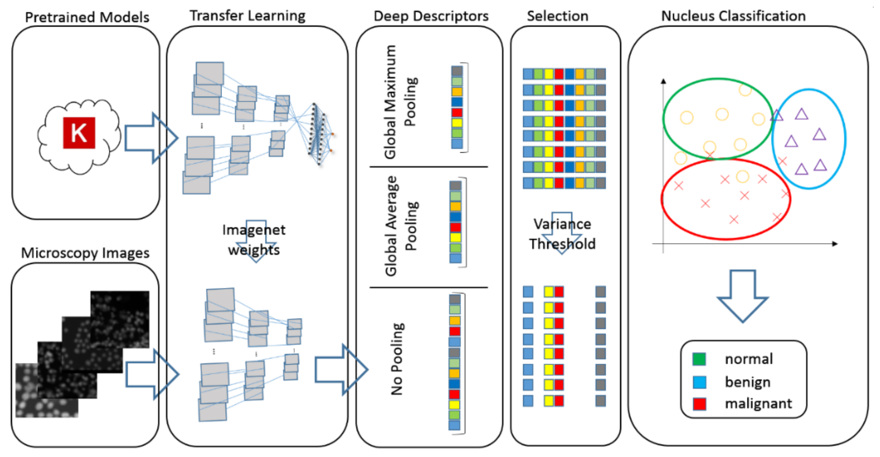
2.4. Deep–Learning Descriptors

2.4.1. Deep–Analysis Specific Image Preprocessing

Deep–learning analysis requires a uniform pixel array dimensionality in vertical and horizontal axes. After the aforementioned data preprocessing by rescaling with respect to the nuclei size as described in Section 2.2, different image sizes were produced. Thus, additional preprocessing steps involving image cropping and padding were applied to ensure the same image size across every sample. Every pretrained model input was set to 250 by 250 pixels. Consequently, original images with higher pixel count were cropped and padded into sub-images to match the aforementioned input. This augmented the examined dataset from 79 to 105 images. The image identifier and nuclei characterization label of the additional 26 images were preserved to avoid compromising the cross-validation process. Therefore, the sample stratification was based on the unique image identifiers.

2.4.2. Transfer Learning Analysis

A transfer learning approach with models pretrained on ImageNet dataset [33] was followed as an “off-the-shelf” feature extraction module. Thus, training of deep models on the examined dataset was avoided since the limited size of the dataset was inappropriate for a de novo network development. In particular, seven families of model architectures with their variations were tested, namely Xception [34], Inception [35], ResNet [36], VGG [37], MobileNet [38], DenseNet [39], NasNet [40]. Their architectural differences in terms of number of layers and learned parameters, type of convolutional kernels and uniqueness of layer organization produced a diverse set of deep imaging descriptors.

The pretrained models were downloaded from the online repository of Keras [41]. The neural and classification layers were omitted because they were trained to differentiate among 1000 classes of natural images. The remaining weights of the convolutional layers were transferred to a new fully convolutional model for feature extraction on fluorescence microscopy images.

Additionally, three different approaches were implemented during feature extraction including raw features from the last convolutional layer of each model, features with global average and global maximum pooling at a kernel level. Following extraction an unsupervised variance-based feature selection process was applied for reducing the dimensionality of the deep vectors. Five thresholds were examined from 0.0 to 0.5 variance at a feature level. The resulted deep descriptors were standardized by value rescaling on a feature-basis prior to classification. Finally, traditional machine learning algorithms (SVM RBF and Logistic Regression) were trained on these deep descriptors to distinguish among normal, benign, and malignant nuclei. A detailed depiction of the overall methodology for the proposed deep analysis is illustrated in Figure 2. The source code of the aforementioned analysis can be found at https://github.com/trivizakis/deepcell (access date: 9 April 2021).

2.5. Ternary Classification

In order to differentiate normal, benign and malignant nuclei images, two classifiers from the scikit-learn library [42] were used; the logistic regression implemented with the one-versus-rest (OVR) scheme and the support vector machine (SVM) with the radial basis function kernel (RBF) for both pathomics and deep descriptors.

Support vector machines (SVM) have been used extensively in medical image classification [43,44] for differentiating tissue by utilizing deep features. In the context of nuclei type differentiation both classifiers were trained in a 10-fold cross-validation scheme on the extracted imaging and deep descriptors. The data stratification was applied on an image identifier basis with respect to the class representation across folds to avoid sample selection bias and overfitted models.

2.6. Model Performance Evaluation Metrics

In order to evaluate the performance of both pathomics and deep learning analyses the mean AUC and ACC with their standard deviations were calculated on the unseen testing sets. In particular, the feature selection for pathomics was based on optimizing the classification accuracy.

3. Results

The examined fluorescence dataset has a class distribution of 51.9% for normal, 12.7% for benign and 35.4% for malignant samples. With varying magnification scales, the original image dimensions ranged from 550 by 430 to 1360 by 1024 pixels. A harmonization process prior to analysis, as defined in Section 2.2 and depicted in Figure 1, was motivated by the need for the nuclei’s shape and texture features to be comparable. Additional cropping and padding were performed to the harmonized images for deep feature extraction to achieve a uniform image shape of 250 by 250 pixels for each of the examined fluorescence image, as shown in Section 2.4.1.

3.1. Pathomics

After the extraction of the 1032 textural and statistical features, a feature selection process was performed with the Minimum Redundancy Maximum Relevance (mRMR) algorithm that identifies the most relevant patterns in the training set. A step size equal to one was used by mRMR to compute the corresponding performances using one up to 50 selected features. However, for the sake of simplicity only indicative performance results for a subset of the used values are reported in

Table 1. Area under the curve score and accuracy (mean ± standard deviation) of classification per number of selected pathomics features for the two classifiers used. The best performance was highlighted with bold.

	Logistic Regression (OVR)		SVM RBF
Selected Features	AUC	ACC	AUC	ACC
3	0.956 ± 0.047	0.8 ± 0.093	0.965 ± 0.056	0.786 ± 0.064
6	0.968 ± 0.033	0.871 ± 0.103	0.954 ± 0.042	0.843 ± 0.118
10	0.983 ± 0.03	0.871 ± 0.128	0.981 ± 0.032	0.843 ± 0.159
20	0.986 ± 0.033	0.957 ± 0.105	0.965 ± 0.086	0.929 ± 0.103
30	0.992 ± 0.019	0.886 ± 0.064	0.978 ± 0.033	0.914 ± 0.035
40	0.996 ± 0.006	0.943 ± 0.049	0.976 ± 0.031	0.871 ± 0.07
50	0.99 ± 0.019	0.943 ± 0.073	0.986 ± 0.033	0.886 ± 0.064

. In more detail, for the case of the logistic regression classifier, the results varied from 0.956 to 0.996 for AUC and 0.8 to 0.957 for ACC. The SVM RBF classifier resulted in AUC values from 0.954 to 0.986 and ACC from 0.786 to 0.929.

3.2. Transfer Learning

The experiments were performed on computational infrastructure featuring a 10-core Xeon processor with 32 gigabytes of RAM and an Nvidia GTX 1070 graphics card with 8 gigabytes of VRAM. The extraction of deep features from a single image requires approximately 14 ms to 426 ms depending on the architecture. Seven deep architecture families with a total of eighteen model variations were examined. The models were trained on ImageNet dataset, the neural network layers were rejected and three methods for extracting the deep features were applied, as described in Section 2.4.2. The “off-the-shelf” feature extractor transfer learning technique includes: (a) preserving convolutional layer weights from the Keras pretrained model, (b) introducing a new input of images of size 250 by 250 pixels, and (c) removing fully connected and Softmax layers (Figure 2). To prevent samples from the same image being used in both the training and testing sets, a stratified 10-fold cross-validation technique was used on a unique image identifier basis.

Additionally, five variance thresholds were integrated ranging from 0.0 to 0.5 significantly reducing the dimensionality of deep descriptors. Finally, traditional machine learning classifiers were trained with a new per deep descriptor labeling for distinguishing among normal, benign, and malignant nuclei, and they were capable of reaching a testing ACC of up to 0.945 ± 0.06. In terms of ACC performance, the Xception (0.923–0.944), Inception (0.916–0.945), and DenseNet (0.916–0.951) were the top performing deep descriptors across all three feature types, as can be observed in

Table 2. Performance of nuclei image characterization is organized by feature type, architecture family, variance threshold and classifier. The best model performance for each feature type was highlighted with italics and the best overall model with bold.

Feature Type	Model Family	SVM RBF			Logistic Regression OVR
		Variance Threshold	ACC	AUC	Variance Threshold	ACC	AUC
Raw	Xception	0.0	0.943 ± 0.07	0.956 ± 0.05	0.0	0.925 ± 0.08	0.944 ± 0.07
	VGG	0.3	0.646 ± 0.09	0.664 ± 0.08	0.5	0.905 ± 0.07	0.925 ± 0.06
	ResNet	0.4	0.876 ± 0.07	0.898 ± 0.07	0.3	0.924 ± 0.10	0.943 ± 0.07
	Inception	0.5	0.916 ± 0.09	0.929 ± 0.07	0.5	0.942 ± 0.06	0.960 ± 0.04
	MobileNet	0.0	0.905 ± 0.09	0.909 ± 0.07	0.0	0.924 ± 0.09	0.941 ± 0.07
	DenseNet	0.1	0.926 ± 0.13	0.940 ± 0.10	0.4	0.944 ± 0.06	0.951 ± 0.05
	NasNet	0.0	0.897 ± 0.10	0.908 ± 0.09	0.0	0.907 ± 0.07	0.926 ± 0.05
Global Maximum	Xception	0.4	0.933 ± 0.06	0.943 ± 0.05	0.2	0.923 ± 0.07	0.944 ± 0.05
	VGG	0.2	0.659 ± 0.06	0.679 ± 0.04	0.1	0.905 ± 0.06	0.922 ± 0.04
	ResNet	0.1	0.876 ± 0.10	0.892 ± 0.10	0.2	0.926 ± 0.11	0.940 ± 0.10
	Inception	0.3	0.918 ± 0.10	0.932 ± 0.10	0.3	0.945 ± 0.07	0.922 ± 0.04
	MobileNet	0.3	0.907 ± 0.08	0.921 ± 0.07	0.4	0.914 ± 0.07	0.934 ± 0.06
	DenseNet	0.5	0.916 ± 0.08	0.933 ± 0.06	0.3	0.951 ± 0.05	0.962 ± 0.04
	NasNet	0.0	0.897 ± 0.08	0.909 ± 0.07	0.2	0.913 ± 0.08	0.926 ± 0.07
Global Average	Xception	0.2	0.944 ± 0.06	0.953 ± 0.06	0.2	0.925 ± 0.08	0.938 ± 0.07
	VGG	0.0	0.763 ± 0.14	0.783 ± 0.13	0.2	0.905 ± 0.09	0.910 ± 0.08
	ResNet	0.1	0.875 ± 0.07	0.896 ± 0.07	0.3	0.942 ± 0.07	0.954 ± 0.06
	Inception	0.3	0.945 ± 0.06	0.959 ± 0.05	0.0	0.935 ± 0.07	0.951 ± 0.06
	MobileNet	0.4	0.913 ± 0.08	0.923 ± 0.07	0.2	0.924 ± 0.07	0.948 ± 0.06
	DenseNet	0.2	0.935 ± 0.06	0.941 ± 0.06	0.4	0.935 ± 0.07	0.948 ± 0.06
	NasNet	0.2	0.915 ± 0.09	0.919 ± 0.09	0.0	0.925 ± 0.07	0.942 ± 0.07

. It is worth noting that models based on the VGG and ResNet families consistently gave an error higher or equivalent (12.3–35.4%) than the benign class distribution despite the higher score of separability (AUC up to 0.896), indicating that these models have likely been biased toward the minority class.

4. Discussion

This study was mainly focused on the classification of a publically available fluorescence dataset. The dataset contained 41 images of normal nuclei of human cells and 38 images of pathological nuclei from three different types of rare pediatric embryonal tumors. Two of them, neuroblastoma and ganglioneuroblastoma, are neuroblastic tumors of different grades of differentiation and malignancy which belong to the group of tumors arising from the sympathoadrenal lineage of the neural crest during development, while the third one, Wilms’ tumor (nephroblastoma) is a malignant embryonal neoplasm derived from nephrogenic blastemal cells. Two different AI pipelines based on pathomics and deep learning were implemented for the automated classification between normal benign and malignant types of nuclei as labelled by the expert. The classification was a challenging task for the AI pipelines since the dataset exhibited significant heterogeneity in terms of vendor, image size, magnification, and signal–to–noise ratio.

The first step of our analysis was to address the heterogeneity in nuclei sizes emanating from different magnifications and image sizes since size and shape related features from the pyradiomics library could potentially introduce exaggerated values not corresponding to actual differences and lead to unreliable results. To overcome this limitation, an adaptive pre-processing technique in Section 2.2 was proposed to ensure that in all images, nuclei sizes fall within a similar size range. This harmonization step was used for both presented ML analyses in order to ensure uniform nuclei image dimensions.

Regarding the classification performance with pathomics feature extraction, we experimentally showed by repeating the classification with a different number of selected features using the pymrmr algorithm, that for 20 selected features the minimum error was achieved, as presented in Table 1 for both classifiers. Additionally, it is noteworthy that when using more than 20 selected features, the performance accuracy drops (Table 1). Despite the heterogeneous nature of the dataset, classification through pathomics analysis exhibited the highest performance with an AUC of 0.986 and an ACC of 0.957 regarding the logistic regression classifier. In a similar way, the SVM RBF classifier performed almost equally to the logistic regression, with slight differences presenting an AUC of 0.965 and an ACC of 0.929.

An additional harmonization pre-processing stage involving image cropping and padding in the DL approach was necessary prior to performing the feature extraction from the pretrained models (Section 2.4.1) to ensure consistent input image size. Due to the small size of the examined dataset, only transfer learning techniques were considered.

The DenseNet consistently achieved the highest performance (up to ACC 0.951 ± 0.05 and AUC 0.962 ± 0.04) regardless of the employed pooling technique, as shown in Table 2. The state-of-the-art performance of the proposed methodology demonstrates the feasibility of DL analysis in fluorescence histology image analysis and modelling despite the limited size of the available data. This encouraging result indicates that AI can be used with advantage to address clinical unmet needs in fluorescence pathology image analysis. To this end, creating larger, labelled and diverse datasets in terms of vendor and image settings is of utmost importance for developing more generalizable and trustworthy AI models in this field.

The pathomics-based models with 3, 6, 10 (LR and SVM RBF) and 40, 50 (SVM RBF) features, as well as the deep descriptors from VGG, ResNet (SVM RBF with all the three types of deep features) in Table 2, may have made biased predictions because the prediction error (12.3–20%, Table 1 and Table 2) is higher or equal to the minority class distribution (12.7%). Regardless of the fact that the classifier seems to be capable of effectively separating samples from the three classes suggested by the high AUC value, the lower accuracy score (ACC) in this case indicates a biased classifier.

Leveraging AI for characterizing vast amounts of pathology image data can spare clinical experts from tedious and time-consuming tasks, thus alleviating their heavy workload. At the same time, the collaboration of humans and AI has the potential to augment the overall efficiency of the decision-making process based on pathology image analysis.

We are aware that our research has some limitations. The first limitation arises from the relatively small size of the dataset used (N = 79 images). That said, the analysis pipeline was carefully selected considering the size of the dataset size, and this was the main reason that more traditional techniques were used. The proposed pipeline should be further evaluated in larger and even more diverse datasets to promote the generalizability of the results. Furthermore, alternative feature selection techniques can be tested in the context of a more extended study. In addition, we are aware that the image pre-processing method involving down sampling could lead to loss of image information, but this step was necessary for the DL models. Lastly, different tissue preparation processes for fluorescence imaging as well as different imaging settings lead to different noise distributions and increased data heterogeneity, posing additional challenges for AI classification algorithms

5. Conclusions

The proposed classification with pathomics and DL methods demonstrated good performance (ACC up to: 0.957 ± 0.105 for pathomics and 0.951 ± 0.05 for DL) on differentiating between normal, benign and malignant nuclei types. These results indicate that the proposed classification scheme is a promising framework for aiding pathology fluorescence image analysis and interpretation. To accelerate the clinical translation of such tools a closer collaboration between AI researchers and clinicians is required. At the same time, the development of a larger fluorescence histology image database is a sine qua non condition for optimizing such DL models and increasing robustness and generalizability.

References

1. Hamad, A.; Ersoy, I.; Bunyak, F. Improving Nuclei Classification Performance in H&E Stained Tissue Images Using Fully Convolutional Regression Network and Convolutional Neural Network. In Proceedings of the 2018 IEEE Applied Imagery Pattern Recognition Workshop (AIPR), Washington, DC, USA, 9–11 October 2018; pp. 1–6. [Google Scholar] [CrossRef]
2. Putzu, L.; Fumera, G. An Empirical Evaluation of Nuclei Segmentation from H&E Images in a Real Application Scenario. Appl. Sci. 2020, 10, 7982. [Google Scholar] [CrossRef]
3. Salvi, M.; Molinari, F. Multi-tissue and multi-scale approach for nuclei segmentation in H&E stained images. Biomed. Eng. Online 2018, 17, 1–13. [Google Scholar] [CrossRef] [Green Version]
4. Lakis, S.; Kotoula, V.; Koliou, G.-A.; Efstratiou, I.; Chrisafi, S.; Papanikolaou, A.; Zebekakis, P.; Fountzilas, G. Multisite Tumor Sampling Reveals Extensive Heterogeneity of Tumor and Host Immune Response in Ovarian Cancer. Cancer Genom. Proteom. 2020, 17, 529–541. [Google Scholar] [CrossRef] [PubMed]
5. Hägele, M.; Seegerer, P.; Lapuschkin, S.; Bockmayr, M.; Samek, W.; Klauschen, F.; Müller, K.-R.; Binder, A. Resolving challenges in deep learning-based analyses of histopathological images using explanation methods. Sci. Rep. 2020, 10, 1–12. [Google Scholar] [CrossRef] [Green Version]
6. Shapcott, M.; Hewitt, K.J.; Rajpoot, N. Deep Learning with Sampling in Colon Cancer Histology. Front. Bioeng. Biotechnol. 2019, 7, 52. [Google Scholar] [CrossRef] [Green Version]
7. Dimitriou, N.; Arandjelović, O.; Caie, P.D. Deep Learning for Whole Slide Image Analysis: An Overview. Front. Med. 2019, 6, 264. [Google Scholar] [CrossRef] [PubMed] [Green Version]
8. Kurc, T.; Bakas, S.; Ren, X.; Bagari, A.; Momeni, A.; Huang, Y.; Zhang, L.; Kumar, A.; Thibault, M.; Qi, Q.; et al. Segmentation and Classification in Digital Pathology for Glioma Research: Challenges and Deep Learning Approaches. Front. Neurosci. 2020, 14, 27. [Google Scholar] [CrossRef] [PubMed] [Green Version]
9. Barisoni, L.; Lafata, K.J.; Hewitt, S.M.; Madabhushi, A.; Balis, U.G.J. Digital pathology and computational image analysis in nephropathology. Nat. Rev. Nephrol. 2020, 16, 669–685. [Google Scholar] [CrossRef]
10. Yetiş, S.Ç.; Çapar, A.; Ekinci, D.A.; Ayten, U.E.; Kerman, B.E.; Töreyin, B.U. Myelin detection in fluorescence microscopy images using machine learning. J. Neurosci. Methods 2020, 346, 108946. [Google Scholar] [CrossRef]
11. Unger, J.; Hebisch, C.; Phipps, J.E.; Lagarto, J.L.; Kim, H.; Darrow, M.A.; Bold, R.J.; Marcu, L. Real-time diagnosis and visualization of tumor margins in excised breast specimens using fluorescence lifetime imaging and machine learning. Biomed. Opt. Express 2020, 11, 1216–1230. [Google Scholar] [CrossRef]
12. Held, M.; Schmitz, M.H.A.; Fischer, B.; Walter, T.; Neumann, B.; Olma, M.H.; Peter, M.; Ellenberg, J.; Gerlich, D.W. Cell Cognition: Time-resolved phenotype annotation in high-throughput live cell imaging. Nat. Methods 2010, 7, 747–754. [Google Scholar] [CrossRef] [PubMed] [Green Version]
13. Alvarez-Jimenez, C.; Sandino, A.A.; Prasanna, P.; Gupta, A.; Viswanath, S.E.; Romero, E. Identifying Cross-Scale Associations between Radiomic and Pathomic Signatures of Non-Small Cell Lung Cancer Subtypes: Preliminary Results. Cancers 2020, 12, 3663. [Google Scholar] [CrossRef] [PubMed]
14. Rivenson, Y.; Wang, H.; Wei, Z.; de Haan, K.; Zhang, Y.; Wu, Y.; Günaydın, H.; Zuckerman, J.E.; Chong, T.; Sisk, A.E.; et al. Virtual histological staining of unlabelled tissue-autofluorescence images via deep learning. Nat. Biomed. Eng. 2019, 3, 466–477. [Google Scholar] [CrossRef] [PubMed] [Green Version]
15. Wang, H.; Rivenson, Y.; Jin, Y.; Wei, Z.; Gao, R.; Günaydın, H.; Bentolila, L.A.; Kural, C.; Ozcan, A. Deep learning enables cross-modality super-resolution in fluorescence microscopy. Nat. Methods 2019, 16, 103–110. [Google Scholar] [CrossRef] [PubMed]
16. Li, Y.; Xu, F.; Zhang, F.; Xu, P.; Zhang, M.; Fan, M.; Li, L.; Gao, X.; Han, R. DLBI: Deep learning guided Bayesian inference for structure reconstruction of super-resolution fluorescence microscopy. Bioinformatics 2018, 34, i284–i294. [Google Scholar] [CrossRef]
17. Ouyang, W.; Aristov, A.; Lelek, M.; Hao, X.; Zimmer, C. Deep learning massively accelerates super-resolution localization microscopy. Nat. Biotechnol. 2018, 36, 460–468. [Google Scholar] [CrossRef]
18. Zhou, H.; Cai, R.; Quan, T.; Liu, S.; Li, S.; Huang, Q.; Ertürk, A.; Zeng, S. 3D high resolution generative deep-learning network for fluorescence microscopy imaging. Opt. Lett. 2020, 45, 1695–1698. [Google Scholar] [CrossRef]
19. Oszutowska-Mazurek, D.; Parafiniuk, M.; Mazurek, P. Virtual UV Fluorescence Microscopy from Hematoxylin and Eosin Staining of Liver Images Using Deep Learning Convolutional Neural Network. Appl. Sci. 2020, 10, 7815. [Google Scholar] [CrossRef]
20. Spilger, R.; Wollmann, T.; Qiang, Y.; Imle, A.; Lee, J.Y.; Müller, B.; Fackler, O.T.; Bartenschlager, R.; Rohr, K. Deep Particle Tracker: Automatic Tracking of Particles in Fluorescence Microscopy Images Using Deep Learning. Lect. Notes Comput. Sci. 2018, 128–136. [Google Scholar] [CrossRef]
21. Jang, H.-J.; Song, I.H.; Lee, S.H. Generalizability of Deep Learning System for the Pathologic Diagnosis of Various Cancers. Appl. Sci. 2021, 11, 808. [Google Scholar] [CrossRef]
22. Valieris, R.; Amaro, L.; Osório, C.A.B.D.T.; Bueno, A.P.; Mitrowsky, R.A.R.; Carraro, D.M.; Nunes, D.N.; Dias-Neto, E.; da Silva, I.T. Deep Learning Predicts Underlying Features on Pathology Images with Therapeutic Relevance for Breast and Gastric Cancer. Cancers 2020, 12, 3687. [Google Scholar] [CrossRef]
23. Kromp, F.; Bozsaky, E.; Rifatbegovic, F.; Fischer, L.; Ambros, M.; Berneder, M.; Weiss, T.; Lazic, D.; Dörr, W.; Hanbury, A.; et al. An annotated fluorescence image dataset for training nuclear segmentation methods. Sci. Data 2020, 7, 1–8. [Google Scholar] [CrossRef] [PubMed]
24. Shimada, H.; Ambros, I.M.; Dehner, L.P.; Hata, J.; Joshi, V.V.; Roald, B. Terminology and morphologic criteria of neuroblastic tumors: Recommendations by the International Neuroblastoma Pathology Committee. Cancer 1999, 86, 349–363. [Google Scholar] [CrossRef]
25. Moch, H.; Cubilla, A.L.; Humphrey, P.A.; Reuter, V.E.; Ulbright, T.M. The 2016 WHO Classification of Tumours of the Urinary System and Male Genital Organs—Part A: Renal, Penile, and Testicular Tumours. Eur. Urol. 2016, 70, 93–105. [Google Scholar] [CrossRef] [PubMed]
26. Uhl, A.; Wimmer, G. A systematic evaluation of the scale invariance of texture recognition methods. Pattern Anal. Appl. 2015, 18, 945–969. [Google Scholar] [CrossRef] [Green Version]
27. Coelho, L.P. Mahotas: Open source software for scriptable computer vision. J. Open Res. Softw. 2013, 1, e3. [Google Scholar] [CrossRef]
28. Duron, L.; Balvay, D.; Perre, S.V.; Bouchouicha, A.; Savatovsky, J.; Sadik, J.-C.; Thomassin-Naggara, I.; Fournier, L.; Lecler, A. Gray-level discretization impacts reproducible MRI radiomics texture features. PLoS ONE 2019, 14, e0213459. [Google Scholar] [CrossRef]
29. Le, N.Q.K.; Hung, T.N.K.; Do, D.T.; Lam, L.H.T.; Dang, L.H.; Huynh, T.-T. Radiomics-based machine learning model for efficiently classifying transcriptome subtypes in glioblastoma patients from MRI. Comput. Biol. Med. 2021, 132, 104320. [Google Scholar] [CrossRef] [PubMed]
30. Le, N.Q.K.; Do, D.T.; Chiu, F.-Y.; Yapp, E.K.Y.; Yeh, H.-Y.; Chen, C.-Y. XGBoost Improves Classification of MGMT Promoter Methylation Status in IDH1 Wildtype Glioblastoma. J. Pers. Med. 2020, 10, 128. [Google Scholar] [CrossRef]
31. Van Griethuysen, J.J.; Fedorov, A.; Parmar, C.; Hosny, A.; Aucoin, N.; Narayan, V.; Beets-Tan, R.G.; Fillion-Robin, J.-C.; Pieper, S.; Aerts, H.J. Computational Radiomics System to Decode the Radiographic Phenotype. Cancer Res. 2017, 77, e104–e107. [Google Scholar] [CrossRef] [Green Version]
32. Peng, H.; Long, F.; Ding, C. Feature selection based on mutual information criteria of max-dependency, max-relevance, and min-redundancy. IEEE Trans. Pattern Anal. Mach. Intell. 2005, 27, 1226–1238. [Google Scholar] [CrossRef] [PubMed]
33. Deng, J.; Dong, W.; Socher, R.; Li, L.-J.; Li, K.; Fei-Fei, L. ImageNet: A large-scale hierarchical image database. In Proceedings of the 2009 IEEE Computer Society Conference on Computer Vision and Pattern Recognition Workshops, Miami, FL, USA, 20–25 June 2009; pp. 248–255. [Google Scholar]
34. Chollet, F. Xception: Deep Learning with Depthwise Separable Convolutions. In Proceedings of the IEEE Conference on Computer Vision and Pattern Recognition (CVPR), Honolulu, HI, USA, 21–26 July 2017; pp. 1251–1258. [Google Scholar]
35. Szegedy, C.; Vanhoucke, V.; Ioffe, S.; Shlens, J.; Wojna, Z. Rethinking the inception architecture for computer vision. Conf. Proc. 2016, 2818–2826. [Google Scholar] [CrossRef] [Green Version]
36. He, K.; Zhang, X.; Ren, S.; Sun, J. Deep Residual Learning for Image Recognition. In Proceedings of the 2016 IEEE Conference on Computer Vision and Pattern Recognition (CVPR), Las Vegas, NV, USA, 27–30 June 2016; pp. 770–778. [Google Scholar]
37. Simonyan, K.; Zisserman, A. Very deep convolutional networks for large-scale image recognition. arXiv 2014, preprint. arXiv:1409.1556. [Google Scholar]
38. Howard, A.G.; Zhu, M.; Chen, B.; Kalenichenko, D.; Wang, W.; Weyand, T.; Andreetto, M.; Adam, H. Mobile Nets: Efficient Convolutional Neural Networks for Mobile Vision Applications. arXiv 2017, arXiv:1704.04861. [Google Scholar]
39. Huang, G.; Liu, Z.; van der Maaten, L.; Weinberger, K.Q. Densely Connected Convolutional Networks. In Proceedings of the 2017 IEEE Conference on Computer Vision and Pattern Recognition (CVRP), Honolulu, HI, USA, 21–26 July 2017; pp. 4700–4708. [Google Scholar]
40. Zoph, B.; Vasudevan, V.; Shlens, J.; Le, Q.V. Learning Transferable Architectures for Scalable Image Recognition. In Proceedings of the 2018 IEEE conference on computer vision and pattern recognition (CVRP), Salt Lake City, UT, USA, 18–23 June 2018; pp. 8697–8710. [Google Scholar]
41. Chollet, F. Others Keras, an Open Library for Deep Learning. Available online: http://citebay.com/how-to-cite/keras/ (accessed on 9 April 2021).
42. Pedregosa, F.; Varoquaux, G.; Gramfort, A.; Michel, V.; Thirion, B.; Grisel, O.; Blondel, M.; Prettenhofer, P.; Weiss, R.; Du-Bourg, V.; et al. Scikit-learn: Machine Learning in Python. J. Mach. Learn. Res. 2011, 12, 2825–2830. [Google Scholar]
43. Trivizakis, E.; Manikis, G.C.; Nikiforaki, K.; Drevelegas, K.; Constantinides, M.; Drevelegas, A.; Marias, K. Extending 2-D Convolutional Neural Networks to 3-D for Advancing Deep Learning Cancer Classification with Application to MRI Liver Tumor Differentiation. IEEE J. Biomed. Heal. Inform. 2018, 23, 923–930. [Google Scholar] [CrossRef] [PubMed]
44. Trivizakis, E.; Ioannidis, G.S.; Melissianos, V.D.; Papadakis, G.Z.; Tsatsakis, A.; Spandidos, D.A.; Marias, K. A novel deep learning architecture outperforming ‘off-the-shelf’ transfer learning and feature-based methods in the automated assessment of mammographic breast density. Oncol. Rep. 2019, 42, 2009–2015. [Google Scholar] [CrossRef] [Green Version]
Figure 1. Workflow for image pre−processing. ”A” denotes the mean nucleus size/area of the current image, ”M” the minimum mean nucleus area of all images and “ϵ”denotes a small number of pixels.
Applsci 11 03796 g001
Figure 2. Pretrained models from the Keras repository were leveraged for the proposed deep learning analysis, specifically in feature extraction. The unsupervised threshold-based feature selection process was followed by a classifier, either SVM RBF or logistic regression.
Applsci 11 03796 g002