Abstract
Carbonate rocks are considered to be essential reservoirs for human development, but are known to be highly heterogeneous and difficult to fully characterize. To better understand carbonate systems, studying pore-scale is needed. For this purpose, three blocks of carbonate rocks (chalk, enthrocal limestone, and dolomite) were cored into 30 samples with diameters of 18 mm and lengths of 25 mm. They were characterized from pore to core scale with laboratory tools. These techniques, coupled with X-ray micro-tomography, enable us to quantify hydrodynamic properties (porosity, permeability), elastic and structural properties (by acoustic and electrical measurements), pore distribution (by centrifugation and calculations). The three rocks have similar properties to typical homogeneous carbonate rocks but have specific characteristics depending on the rock type. In the same rock family, sample properties are different and similarities were established between certain measured properties. For example, samples with the same hydrodynamic (porosity, permeability) and structural (formation factor, electrical tortuosity) characteristics may have different elastic properties, due to their cohesion, which itself depends on pore size distributions. Microstructure is understood as one of the essential properties of a rock and thus must be taken into account to better understand the initial characteristics of rocks.
1. Introduction
Carbonate formations are considered to be useful reservoirs for human development. They are often used for their resources such as water, oil and gas, but also for their storage capacity or their ability to heat, such as in geothermal energy [1,2]. It is essential to comprehend the properties of these reservoirs in order to operate them in a sustainable and responsible way. Carbonate rocks are known to be highly heterogeneous, with varying properties at different scales. They are known as a complex medium, due to their formation of component particles in matrixes composed of cement and/or limestone mud [3,4,5,6]. Variabilities in microstructure lead to difficulties in reservoir characterization. Studying pore scale is need to understand carbonate systems. Rock structure is adequately characterized by measuring and calculating properties at pore scale [7,8,9,10]. Furthermore, once the structural-property relationships are identified at pore scale they can be replicated at large scale, therefore facilitating large scale reservoir characterization.
Two factors are essential in rock characterization: solid structure [11] and porosity [3]. Indeed, geometry and arrangements of pores are crucial features in the comprehension of reservoir structure and its characterization [5,12]. Different techniques are used to characterize pore arrangement and associated petrophysical properties. Seismic properties are known to be strongly affected by microstructure and grain contacts. Measurements of P and S waves velocities by current injection in rock are therefore very interesting for structure characterization [7]. Indeed, porosity is considered the most important parameter in controlling elastic wave velocities, as it increases when velocities decrease [10]. Otherwise, hydrodynamic and transport properties are controlled by the pores’ geometry, connectivity (i.e., general availability of pathways for transport [13]) and network architecture. Indeed, the electric current is conducted by the saturating fluid present in the connected poral phase of the rock. Then, properties can be deduced from electrical resistivity measurements, using empirical resistivity-porosity [14] and porosity-permeability relationships (Kozeny-Carman’s equations, [15,16]). Archie’s law is used at various investigation scales and relates porosity to rock resistivity through the formation factor and the cementation index. Even if this equation is proven to be more efficient on sandstones rocks, there is no better law to characterize carbonate rocks. Tortuosity, which is assimilated to connectivity of the poral phase, is also deduced from rock resistivity [17,18,19]. Constrictivity (i.e., parameter related to bottleneck effect in pores [20]) is also one of the related parameter which is mostly neglected as it is very complicated to evaluate. Nevertheless, a recent study [21] demonstrates that constrictivity can be used to better estimate the tortuosity. Permeability is also given to strongly control hydrodynamic properties, and can be estimated from the combination of several parameters, such as grain diameters, critical pore size and specific surface [15,16,22,23,24].
On multiple discrete carbonate samples from two different areas, it has been shown that acoustic velocity depends on porosity and predominant pore type [25]. P and S waves velocities are known to be affected by the age of carbonate rocks, as well as by the porosity type [7]. For example, higher velocities are found in samples with dominant moldic and interfossil porosity than with dominant interparticle and microporosity [7]. Analyses of texture, mineralogy and acoustic properties carried out on dry and saturated samples show that in granular rocks, the shear modulus decreases with saturation, contrary to crystalline and cemented carbonates [26]. The combining effect of microporosity, pore network complexity and pore size are also considered to be very influent for acoustic velocities [27] and electrical resistivity [8,28]. This infers that samples with large simple pores and few microporosity display higher P and S waves velocities, as well as higher cementation factors than samples with small and complicated pores [27]. Concerning chalk specifically, P and S waves have been studied based on porosity and pore fluid saturation at three different scales [29]. A power law between porosity and formation factor in cracked mylonite is then found [30]. Studies of pore level heterogeneity on petrophysical properties on carbonates cores have shown that much of the porosity is dominated by microporosity, and that large intergranular pores are responsible for increasing permeability and decreasing electrical conductivity [31]. Electrical microscopic parameters are highly influenced by micro and centimetric scale heterogeneity [9]. Limestone rock porosity and permeability are also controlled by pore shapes and sizes [32,33]. By dissolving carbonate rock samples, structural parameters such as tortuosity and network geometry control changes in porosity and permeability [34,35]. Thus, characterizing the pore structure is also crucial in predicting dissolution rate and localization.
At pore scale, 3D image analysis is very useful to save time and to study the hydrodynamic parameters of rocks without destructing them [27]. However, the pixel size is a discriminant parameter, especially for rocks with many small pores, such as carbonates rocks and particularly chalk. This technique, paired with laboratory analysis, yields a more complete characterization of rocks [33], including pore distribution determination [36]. Porosity, permeability and pore shape can be studied on 2D slices [27] and 3D samples [32,33,37], as well as structural properties [9]. Most of these studies are conducted on one rock type and take into account some existing petrophysical parameters. Relationships between properties are therefore limited to few petrophysical parameters, which imply an incomplete rock characterization.
Consequently, in order to better characterize carbonate reservoirs at various scales, the identification of relevant relationships between measured and calculated properties is essential in order to determine which are the most efficient and necessary. For this purpose, about thirty samples from three carbonates types have been selected: chalk, entrochal limestone and dolomite. Laboratory petrophysical measurements and imaging calculations were performed at core scale and then compared to large scale data.
2. Materials and Methods
2.1. Rocks Presentation
Approximately 30 samples of 18 mm diameter and 20–30 mm length were cored in three carbonate types. They were all surrounded by epoxy resin and PVC pipe for a global diameter of 25 mm, i.e., one inch. A set of 11 samples comes from a cave near Le Havre, Normandie, north-western France. It is characterized by a flint chalk from the lower Senonian and will be called Normandie (labeled N) in the following text. Samples have porosity between 27% and 40% and permeability around 10 mD. A set of 8 samples was cored in a crinoidal limestone from the Oxfordian, from Euville quarry near Nancy, north-eastern France. It will be called Euville (labeled E), and presents porosity around 12% and permeability between 1 and 25 mD. A last set of 12 samples was cored in the Lexos quarry near Toulouse, south-western France. It is a reddish recrystallized limestone from the Bajocian that has been dolomitized. It will be named Lexos (labeled L), and has porosity between 12% and 20% and permeability under 10 mD.
X-ray Diffraction (XRD) on a Bruker D8 Discover shows that Normandie and Euville rocks are exclusively composed of calcite (CaCO), whereas Lexos rocks are composed of dolomite (MgCO). X-ray Fluorescence (XRF) displays clay traces in Normandie, iron traces in Euville. Lexos has a dolomite initial formula of CaMg(CO), with manganese and iron traces. Scanning Electron Microscopy (SEM) on a FEI Quanta 200 FEG displays different pores size for each rock type. Normandie has the smallest pores with diameters under 0.1 mm. Euville has the largest with pores around 0.3 mm diameter. Lexos has medium pores, as it can be seen in Figure 1.
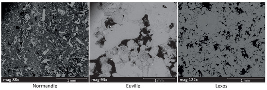
Figure 1.
Images obtained by SEM: Normandie (left), Euville (middle) and Lexos (right).
2.2. Petrophysical Properties from Laboratory Measurements
Petrophysical measurements have been carried out on dry and saturated samples. Samples have been saturated with four different fluids in chemical equilibrium with rocks at four NaCl concentrations: 0.3 mol/L, 0.2 mol/L, 0.1 mol/L and 0.05 mol/L. Between each saturation, they were dried in an oven.
Gas porosity and permeability were measured on dry samples by helium injection using a porosimeter and permeameter. Liquid porosity was measured on saturated samples using a double-weighing on saturated and dried samples, knowing the samples dimensions. Liquid permeability was measured on saturated samples in an experimental device, knowing the differential pressure and using Darcy law. Gas permeability was not performed on dolomite samples, and liquid permeability was only carried out on some of the samples, due to technical issues.
Mechanical properties were carried out with non-destructive acoustic methods, by impulsing ultrasonic frequency waves of 500 kHz into samples between two piezoelectrical transducers. P waves velocities were measured on dry and saturated samples, while S waves velocities were obtained on saturated samples only. Poisson coefficients, Young, Bulk and Shear modulus have been deduced (Equations (1) and (2)) [38,39] with:
where and are respectively the velocities of P and S waves (m/s), K is the Bulk moduli (Pa), G the Shear moduli (Pa), and the bulk density (kg/m).
Structural properties were calculated based on non-destructive electrical methods, consisting of injecting a current into the saturated sample and determining the impedance Z of the sample. Rock conductivity (Equation (3)) and formation factor F (Equation (4)) can be deduced from [40]:
where L is the sample length (m), S is the surface of infiltration (m), is the saturation fluid conductivity (S/m), is the surface conductivity (S/m) which is usually considered null in rocks without clay. Cementation index m (Equation( 5)) [14] and electrical tortuosity (Equation (6)) [19] can then be calculated from:
where is the porosity (%). In order to verify the measurements reproducibility, they have been done before and after each saturation.
Finally, pores size characterization was performed by centrifugation, on samples longer than 20 mm. The method used [41] basically consists of saturating samples and putting them in centrifugation during a given time at increasing velocities [35]. For each specific angular velocity (rad.s), a corresponding air-water capillary pressure h (kPa) is applied to the rock, as Equation (7) [41] shows:
where a is a constant value equal to 9.807 kPa.m, g is the acceleration of gravity (9.81 μm.s), L is the sample length (m) and is the distance between the centrifuge rotation center and the external face of the sample (m). Equivalent pore diameters d (m) are calculated from Young-Laplace equation, based on the air-water capillary pressure h (Equation (8)):
where is the interfacial surface tension between water and air (0.07197 N.m) and is the contact angle, which equals 40° for limestone [42]. A weighing is done after each cycle of velocity in order to determine the water loss and deduce the proportion of a given range of pores size. In this study, velocities used are from 32 to 471 rad/s, which corresponds to pores sizes from approximately 100 to 0.5 μm.
2.3. Petrophysical Properties Computed from Micro-Tomography Images
X-ray micro-tomography (XRMT) was performed on 15 samples over the three samples sets. XRMT is a non-destructive imagery technique. A 3D volume of a studied sample is generated from a set of 2D X-ray attenuation images. In porous media, X-ray energy attenuation depends on crossed phases (voids or solids). The final image is displayed in normalized grey levels, where lighter colors stand for solids and darker colors represent voids. The shades of grey denote the difference in grain density, which can be due to variable mineralogy, or in case of mono-mineral samples, to micro-porosity.
2.3.1. X-ray Tomography Data Acquisition
All the samples have been imaged using a X-ray Computed Tomography (XRCT) scanner (EasyTom 150) at the Institute of Evolution Sciences of Montpellier (ISEM), Montpellier, France, except N04. The pixel size is 12 μm. N04 has been imaged using a XRCT scanner (Bruker Skyscan 1172) at the laboratory unit of Development of EXperimental Methodologies (DMEX), Pau, France. For this sample, the pixel size is 10 μm.
2.3.2. X-ray Tomography Data Processing
After image acquisition, treatments were made before computing rock parameters. They were carried out on a homemade imaging software, previously developed and used [43]. Filters to smooth the pixels histogram (mean filter) and to correct brightness were applied to improve images quality. Then, a segmentation based on a region growing method was used to isolate the void phase of the image. In mono-mineral media, two or three phases are usually observed: the void phase (which can be divided into the macropores phase and the micro-phase, composed of micropores and micro-grains) and the matrix. The macropores phase is composed of pores larger than the pixel size while the micropores and micro-grains smaller than the pixel size are part of the micro-phase. In this study, as previously shown in Figure 1, Normandie has smaller pores than Lexos, which has smaller pores than Euville. In Figure 2, a 2D slice of each rock type is shown. The three structures are very different: Normandie presents a lot of micropores, Euville displays heterogeneous macro-pores, while Lexos shows some homogeneous macro-pores with micropores around. The software used can only display a two-phase segmentation. One phase is composed of macropores (pores larger than the pixel size) while the other phase is considering to be matrix. This segmentation gives a porosity based on macropores, labeled , which is consequently largely underestimated. However, adding micropores (pores smaller than 12 m) with macropores will induce the incorporation of micro-grains into the void phase, and the corresponding porosity () will be consequently overestimated. Calculations have been made on images segmented with the macro-porosity. In order to obtain a consistent segmentation, the macro-void porosity has been correlated with the porosity from the centrifugation calculations. The pores proportion with a diameter smaller than 12 μm allow us to know the proportion of the porosity which is not visible on the images.
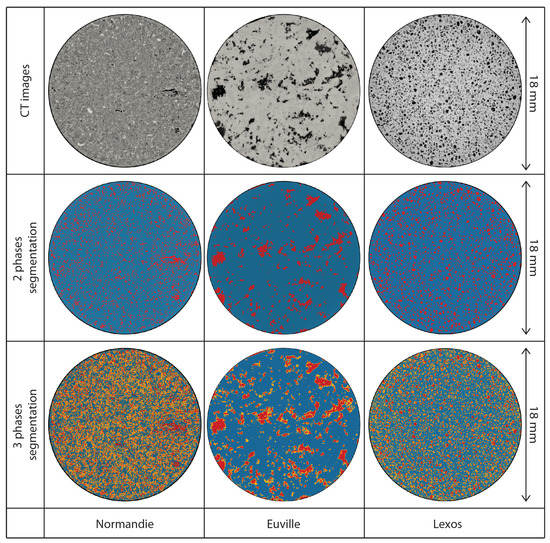
Figure 2.
2D slices obtained from 3D XRMT images. Blue color represents the matrix phase, red the macro-phase and orange the micro-phase.
Once segmentation is complete, calculations can be executed. Porosity, from the macro-phase and micro-phase, is calculated from the segmentation step. Permeability is calculated from skeleton determination, which corresponds to the path that links the center of each connected pore. The time spent to path through the sample is measured. From this skeleton, the hydraulic tortuosity is calculated [15] and displayed in Equation (9). It has been shown that and (seen in Equation (6)) are similar and comparable [19,44].
where is the effective path length and l is the sample length. From the tortuosity, the formation factor (Equation (4)) and the cementation index (Equation (5)) can be deduced.
The software can also compute some parameters that cannot be obtained by non-destructive laboratory techniques. The pore volume and the pore surface are computed, which corresponds to the void-rock interface. By dividing the pore surface by the pore volume (), a relative pore size is given. A high ratio states for an intricate pore system [15] and a huge quantity of small pores. Moreover, pore size distribution is displayed by two probabilistic methods. The first one is based on the insertion of increasing chord lengths into the void phase [36]. The other method is on the insertion of spheres which have a diameter of one pixel. The sphere size is increasing until it touches the matrix, and the software counts the number of spheres of a given size that fit into the pores, and outputs a pore size distribution. Finally, statistics calculations on connected components allow knowing the proportion of the percolating phase into the volume sample (), which is equivalent to the proportion of the sample used by a fluid to pass through.
3. Results
3.1. Petrophysical Properties from Laboratory Measurements
Laboratory measurements were reproduced several times for reproducibility. As the standard deviation is always lower than 2% whatever the parameter measured, the mean value has been chosen as the representative one. Results for gas porosity (), liquid porosity (), gas permeability (), liquid permeability () electrical parameters such as formation factor (), cementation index () and electrical tortuosity (), and acoustical parameters such as P and S waves velocities ( and ), Bulk and Shear moduli (K and G) are summarized in Table 1. To facilitate the explanations and interpretations of the results, only one porosity type will be kept. As expected, gas porosity and permeability are always slightly higher than liquid measurements. Porosity measured by triple weighing has been chosen because samples are more often saturated during measurements and both results are similar. For permeability, Klinkenberg effect is responsible for the differences between the two measurements [45], and gas permeability will be used as a reference here.

Table 1.
Petrophysical parameters summary from laboratory measurements: gas porosity (%), liquid porosity (%), gas permeability (mD), liquid permeability (mD), formation factor , cementation index and electrical tortuosity , P wave velocity (km/s), S wave velocity (km/s), Bulk modulus K (GPa), Shear modulus G (GPa). Imaged samples are identified in bold. The • symbol indicates no measured data.
Table 1 shows that the three rock types present significant differences. Differences in porosity and structural properties (, ) can be easily observed in Figure 3. Samples are displayed depending on their porosity and formation factor, with indications about cementation index. Generally, low porosity induces high formation factor. Normandie presents the highest porosity and lowest formation factor, Euville the opposite and Lexos is in between. They are all situated between the and lines, corresponding to carbonate rocks [4,31]. With the lowest tortuosity, Normandie presents the best connectivity due to high permeability and low tortuosity, while Euville has the highest tortuosity and Lexos is again comprised in between.
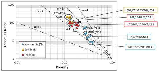
Figure 3.
Crossplot of formation factor over porosity depending on the rock type. Diamonds are for Normandie, squares for Euville and circles for Lexos. Lines of equal cementation factors according to Archie’s law (Equation (5)) are also displayed.
Concerning mechanical properties ( and ) displayed in Table 1, the lowest velocities correspond to the highest porosities, which is consistent with the literature [46]. Normandie has therefore the lowest . However, Lexos presents higher than Euville for lower porosities. This is due to dolomite rocks characteristics [46]. Also, high are more likely to occur in samples with a high proportion of matrix, and therefore a high cohesiveness. A low proportion of micropores, characterized by a diameter smaller than 10 μm [5], usually induces a high proportion of matrix [7]. Therefore, should be higher in samples with low proportion of micropores. Figure 4 displays the pores sizes distribution of the three rock types, and then the micropores proportion. Normandie presents an unimodal distribution of pore sizes with most of pore diameters smaller than 3.5 μm, averaging 61% ± 8% of the total pores size. Its proportion of micropores is comprised between 62% and 80%. Lexos also has an unimodal distribution with a majority of pores size between 3.2 and 11.5 μm (38% ± 8%). Between 57% and 78% of pores are given to be micropores. As for it, Euville presents a bimodal distribution with pore diameters either larger than 31 μm (33% ± 6%) or either smaller than 1.1 μm (38% ± 11%). Proportion of micropores ranges from 47% to 63%. Euville is the rock type with the lowest proportion of micropores.
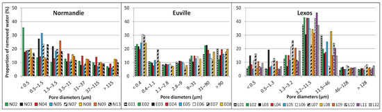
Figure 4.
Pore diameters distribution from the centrifugation measurements. Results for Normandie samples are on the left, Euville in the center, Lexos on the right.
Although samples in each rock type have similar properties, some groups emerge from data. Indeed, Figure 3 display four groups inside Normandie samples, two for Euville and two others for Lexos. These differences in electrical properties (, and ) are explained by differences in mechanical properties (Table 1) and micropores proportions (Figure 4). First concerning Normandie, N02 and N04 present both very low permeabilities (around 5 mD) and very high tortuosities (around 3.7) compared to other samples, so they both present a low connectivity. Also, they both have similar low porosities and high electrical factors, but N02 has lower velocities of P and S waves and higher proportion of micropores than N04 (72% against 62%). N02 is therefore considered to be a less cohesive sample than N04 [7,46]. Then, N08 and N09 present same low porosity, medium electrical properties and micropores proportion (66%), but differ in permeability and . N09 has a lower permeability, which can be related to a higher , inducing a better cohesiveness [46]. Finally, N03, N05, N11 and N13 are part of the group with the highest porosities and lowest electrical factors. However, N03, N05 and N11 have permeabilities around 11 mD while N13 has the double. Moreover, while they all present low , N03 and N05 both have around 80% of micropores while N13 only counts 70%. Therefore, with a higher proportion of large pores, N13 has a less complex poral system than the three others, inducing a better permeability [27].
Despite great similarities, some particularities were found in the Euville samples set. Two groups of samples can emerge from Figure 3 and Table 1 in terms of structural properties: E05/E06/E08 with high electrical factors while the other samples have low electrical factors. However, when looking at , two other groups emerge: E01/E05/E07/E08 with high (around 3.8 km/s) while E02/E03/E04/E06 with low (ranging from 2.3 to 2.7 km/s). Two groups overlap: E05/E08 with high structural factors (, and ) and , and E02/E03/E04 with low ones. E01, E06 and E07 present values which oscillate between the two groups. However, it should be noticed that samples with low permeabilities have high and low proportions of small pores, which is consistent with literature [7,46].
The Lexos samples set seems to present more variability. From Figure 3 and Figure 4, two groups emerge. On one hand, L01, L02, L04, L05, L08, L10 and L11 are samples with high porosities, globally low formation factors. They present more than 60% of pores with sizes comprised between 3.2 and 46 μm, which can be considerate as intermediate size pores. On the other hand, L03, L06, L07, L09 and L12 have low porosities and mainly high formation factors. They also count the highest proportion of micropores (pores with diameters smaller than 10 μm), and especially a lot of very small pores, with more than 40% of pores smaller than 3.2 μm and more than 50% of this proportion is composed of pores smaller than 1.3 μm. In these previous two consistent groups, P-wave velocities differ for samples. In the first group, L02, L04 and L05 present low , which is consistent with high porosities [46] and high proportion of micropores, inducing a low cohesiveness [7]. Contrarily, L01, L08 and L11 have high . For L01 and L08, these high values are correlated with a low proportion of micropores (61 and 57% respectively) compared to other samples which induces a better cohesiveness. However, L11 has a relatively high proportion of micropores (67%), but also has a high value of Bulk modulus K, inducing a low compressibility, which is usually correlated with a high cohesiveness. In the second group, the high proportion of very small pores inducing a low cohesiveness [46] should be consistent with a low [7]. However, only L03 presents a low Vp. L06, L07 and L09 may so have a better cohesiveness, which is not consistent with their high proportion of micropores, but is certainly induced by a low porosity and related to high and Bulk modulus.
Correlations between petrophysical parameters lead us to conclude that the three rock types are to be very different from one another. Normandie and Euville rock samples present similar properties inside each rock type and seem to be homogeneous and defined as a Representative Elementary Volume (REV), even if some particularities can be distinguished. They can be therefore assimilated to representative samples in their rock type, while Lexos rocks properties at pore-scale seem so far too heterogeneous to be representative of its large-scale rock block.
3.2. Petrophysical Calculations from Micro-Tomography Images
Calculations were conducted on micro-tomography images to obtain petrophysical parameters. Two porosities were calculated from the XRMT images, as mentioned in Section 2.3.2. As a reminder, calculations were made on the phase where only macro-void porosity is taken into account. Calculations from the XRMT give values of permeability and hydraulic tortuosity (see Section 2.3.2). From tortuosity, formation factor and cementation index can be deduced (Equations (5) and (6)). All these parameters, as well as the ratio of pore surface over pore volume and the proportion of the percolating volume are displayed in Table 2. Permeability values present fluctuating results due to high sensibility calculations. Changing the segmentation threshold by only one point considerably affects the sample connectivity. Indeed, if, for a given segmentation, a pixel cloggs a path while for another segmentation, this pixel is a pore, the pores organization and the sample connectivity will chang, inducing an increase in permeability. This is mainly why permeability values present such variability, especially for rocks with a majority of small pores such as Normandie. Nevertheless, different segmentations were conducted and porosity values were not strongly affected by a segmentation threshold of one pixel.
Table 2.
Petrophysical parameters summary from tomography images: macro-void porosity (%), total-phase porosity (%), permeability (mD), formation factor , cementation index and hydraulic tortuosity , ratio of pore surface over pore volume and proportion of percolating volume (%). The - stands for non-percolating samples.
From Table 2, Lexos samples display specificity. Regarding L03 and L07 on the imaging software, they do not present percolation path due to the large proportion of pores smaller than 12 μm. Therefore, the connectivity is not visualized on the imaging software. Most of the properties calculated with the sofware, such as macro-void porosity, permeability, electrical factors and the percolating volume , cannot be obtained for these two samples. Tomography analysis has therefore only been conducted on three samples: L01, L04 and L08.
Even if macro-phase porosities are largely underestimated, Normandie presents the highest porosity while Euville and Lexos have lower and similar values. As written above, permeability varies but Normandie displays the highest and Lexos the lowest, with Euville in between. Concerning electrical measurements, Normandie presents the lowest ones, consistently with its high porosity. It also has the lowest variability, except for N04 which has very low values compared to the other samples of the set. It should be highlighted that N04 is the sample imaged with another scanner. Euville has the highest electrical factors and Lexos is comprised between the two others. Pore surface over pore volume is higher for Normandie and Lexos than for Euville. A small is consistent with a low proportion of small pores. The pore size distribution is displayed in Figure 5 with the two calculation methods. It must be noticed that sphere diameters distribution is less relevant for elongated pores than for spherical pores, compared to that of chord lengths. The poral anisotropy can be quantified by chord lengths distributions in X, Y and Z directions, as it can be seen in Figure 6, Figure 7 and Figure 8. X and Y are width directions, while Z direction is longitudinal to the cylinder core direction. Then, in Figure 5, Euville samples always display a low proportion of small pores, while the majority of pores diameters is higher than 120 ΰm, which is consistent with small values of . Finally, Euville, with a proportion of percolating volume higher than 98%, has a very good connectivity in the poral phase. Normandie and Lexos mostly have a good connectivity, except for one Lexos sample with only 55% of percolating and therefore a very low connectivity. At this stage, it should be noticed that data from laboratory measurements and images calculations are in the same order of magnitude and are similar and comparable. A comparison between the two characterization techniques will be done later.
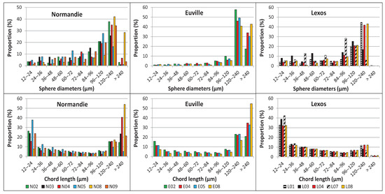
Figure 5.
Pore size distribution obtained by sphere diameters calculations (on the top) and mean chord lengths calculations (on the bottom), using imaging software. Normandie samples are displayed on the left part, Euville on the central part and Lexos is shown on the right.
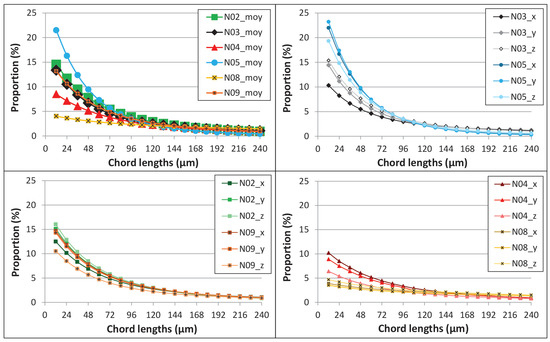
Figure 6.
Chords length distribution for Normandie samples, pore diameters are displayed by proportion. On the top left, an average of chord lengths in the three directions is shown. The rest detail chord lengths in directions X, Y and Z: on the top right, there are N03 and N05, on the bottom left, N02 and N09, while on the bottom right, there are N04 and N08.
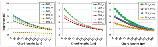
Figure 7.
Chords length distribution for Euville samples, pore diameters are displayed by proportion. On the left, an average of chord lenghts in the three directions is shown. On the middle and right, chord lengths are detailed in directions X, Y and Z: E02 and E04 on the middle and E05 and E08 on the right.
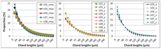
Figure 8.
Chords length distribution for Lexos samples, pore diameters are displayed by proportion. On the left, an average of chord lenghts in the three directions is shown. On the middle and right, chord lengths are detailed in directions X, Y and Z: L01, L04 and L08 on the middle, and L03 and L07 on the right.
In the same way as the previous section, even if samples inside rock types have similar properties, groups can be formed with correlated properties.
Concerning Normanide, two groups emerged from data. With the lowest proportion of , N03 and N05 both have bad-connected poral phase, supported by the lowest permeabilities. They also present a high proportion of small pores with diameters between the pixel size and 36 μm (Figure 5), consistent with their high . Contrarily, N02, N04, N08 and N09 have a very well-connected poral phase. N02 and N09 have moderated permeabilities and , while N04 and N08 are very permeable and have low proportion of small pores, extracted from chord lengths calculations. Inside each couple, N04, N05 and N09 have better connectivity induced by a higher proportion of transverse pores (Figure 6). N04 also has low electrical factors [8,40], which is consistent with a better connection. At this point, it seems important to notice that a low proportion of small pores is consistent with a high permeability [27]. Moreover, it can be noticed that a high proportion of transverse small pores (X and Y directions) is consistent with a low tortuosity.
Concerning Euville, there are no particular couples which appear, they all present very good connected poral phase. However, it can be said that E04 and E08 are very different, while E02 and E05 oscillate between the two, depending on the chosen parameters. Indeed, E04 is the sample with the smallest electrical parameters and the highest permeability, suggesting a good connectivity. There is no significant differences in proportion of pores smaller than 36 μm calculated by sphere diameters distribution (Figure 5), but by chord lengths distribution, E02 counts the highest proportion of small pores, while E08 the lowest. This explains the difference in between E02 and E08. It should be noticed that E02 displays spherical pores, while E05 and E08 have more transverse connections (Figure 7). However, even with more transverse connections, E08 has too few pores in Z directions, implying a very poor permeability and a high tortuosity, which decrease significantly its connectivity.
Finally, Lexos samples present a lot of variability. As written above, L03 and L07 do not present percolation path. This is consistent with their very high , induced by a high quantity of pores around 12 μm, as it has been seen in centrifugation (Section 3.1, Figure 4) and from chord length analysis displayed in Figure 5 and Figure 8. They also have around 25% of pores in Z direction, implying few transverse connections and therefore low connectivity and permeability. The three other samples present disparities although they all three have poor permeability, partly induced by a majority of pores displayed in Z direction (Figure 8). With 55% of percolating volume, permeability lower than 1 mD and high electrical factors, L01 poral phase is poorly connected. Contrarily, L04 and L08 have quite good connectivity, with a better one for L04 according to its higher permeability and lower tortuosity. The three samples still have high , induced by their high proportion of pores diameters smaller than 24 μm in chord length analysis (Figure 5 and Figure 8).
3.3. Comparison between Laboratory Measurements and Tomographic Images Calculations
In this section, the samples only with data obtained from both laboratory measurements and X-ray microtomography are compared.
Whatever the method used, Normandie, Euville and Lexos present the same trend. Generally, Normandie always has the highest porosity, lowest electrical parameters and smallest pore diameters, while Euville is the opposite and Lexos is comprised between them. Nevertheless, parameters are different depending on the method used. Generally, for similar parameters, results from tomographic images calculations have less variability than petrophysical results. This can indicate that the micropores control some of the large scale properties and heterogeneities, but not the macroscopic parameters. Electrical factors are different between laboratory measurements and XRMT calculations with a focus on tortuosity. Electrical tortuosity is obtained from laboratory, while hydraulic tortuosity is from XRMT calculations. The two tortuosities are sometimes considered to be similar [19], while should sometimes be smaller than [44]. In our data set, is higher than . The first hypothesis to explain this difference is that XRMT calculations do not take the microphase in consideration. However, the fluid mainly flows through the connected macropores, and high values of in Table 2 show that there is a good connectivity in the macrophase. The second hypothesis is that the calculation for (using Equation (6)) is wrong. Clennell equation is a simplification of the real expression where f is the constrictivity factor, depending on the pore radius fluctuation ratio. f is comprised between 0 (e.g., trapped pores) and 1 (e.g., cylindrical pores with constant radius), and is taken to be equal to 1 for convenient in Equation (6) and in many other papers. An estimation of f for our samples is made with the hypothesis that [21]. Results are displayed in Table 3. As expected, f values are mainly not equals to 1. When samples have f closed to 0, it means that macropores are poorly connected or that the connection is possible by micropores non-visible in tomography. At the contrary, when f is closed to 1, macropores are well connected and the macrophase is mainly responsible for the fluid flow. Concerning Normandie, once again three groups are shown. N02/N04 have f closed to 0, N03/N05 have f closed to 1, and N08/N09 have f∼0.4. Euville samples are homogeneous and have f∼0.4. This means that pore diameters are subjected to vary a lot inside the sample, inducing a difficult fluid flow. This variation in pore diameters were seen in centrifuge (Figure 4). Lexos samples present high variability, making an interpretation difficult. Nevertheless, we can conclude that constrictivity plays an important role in the rock characterization and should be taken into account.
Table 3.
Estimation of the constrictivity f from electrical tortuosity and hydraulic tortuosity .
The others global variabilities observed between Table 1 and Table 2 are due to the difference between the two poral phase studied. Indeed, XRMT calculations were made based on pores larger than 12 μm, while laboratory measurements were conducted on the global poral phase. For Normandie and Lexos samples, pores larger than 12 μm contribute to only 20 to 40% of the poral phase and constitutes around 50% for the Euville samples. However, even without taking into account a large proportion of poral phase, results from the two methods are similar and consistent, which leads us to conclude that large pores are more likely to control rock parameters on large scale, while small pores may control interactions between parameters at small scale.
Groups formed inside each rock family overlap, from laboratory measurements and XRMT calculations. Indeed, in the Normandie set, N03/N05 couple has been constituted from both methods. This group presents high porosities and low electrical parameters from laboratory measurements, while relatively low permeabilities from XRMT. It also has a high proportion of small pores, which do not participate to the main flow, and is consistent with relatively low percolating volume and , while high f. Then, N02/N09 and N04/N08 formed two groups that can be gathered in one. These samples have relatively low porosities and high electrical factors from laboratory measurements, while high permeabilities from XRMT. They count a relatively low proportion of pores smaller than 10 μm, which comes with a high and , while a low f. In Figure 9, pore diameters distributions from both laboratory measurements and XRMT calculations are displayed on a similar graph. Data from centrifuge are more precise for pores smaller than 30 μm because large pores are more likely to empty before the experiment starts. Concerning XRMT calculations, only pores larger than a pixel are taken into account for calculations, then data is more precise for pores larger than two pixels, i.e., 24 μm. Therefore, in Figure 9, classes up to 30 μm are data from centrifuge and classes up to 30 μm are data from XRMT calculations. The previous mentioned groups are consistent with whatever the method used.
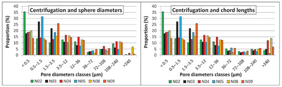
Figure 9.
Pore diameters distributions from laboratory and XRMT calculations for Normandie rock type. Distribution from centrifugation and sphere diameters analysis is displayed on the left, while distribution from centrifugation and chord lengths analyses is shown on the right.
For Euville rocks, as previously established, all samples have very similar properties, whatever the method used. While two couples have been distinguished from laboratory measurements, there is no particular couples constituted from XRMT calculations. Despite E02/E04 always have higher porosities and lower electrical factors than E05/E08, other parameters do not present such variations. Also, pore diameters distribution are pretty much the same, as it can be seen in Figure 10. We can thus conclude that Euville samples have similar properties whatever the technique and scale analyses, indicating that they can be considered to be a Representative Elementary Volume (REV), and can act as analogous to limestone rock reservoirs.
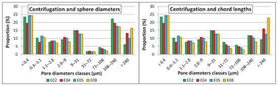
Figure 10.
Pore diameters distributions from laboratory and XRMT calculations for Euville rock type. Distribution from centrifugation and sphere diameters analysis is displayed on the left, while distribution from centrifugation and chord lengths analyses is shown on the right.
Concerning Lexos samples, two groups have been distinguished from images analysis due to the very important proportion of pores diameters smaller than 12 μm in L03 and L07, which induces an impervious barrier to the fluid flow. Two groups have also been formed from the petrophysical analysis, where L01, L04 and L08 have a majority of intermediate size pores and L03/L07 have a majority of pores smaller than 1.3 μm, as displayed in Figure 11. Lexos samples have a majority of pore diameters around 12 μm (Figure 4) and should have equivalent results from laboratory and XRMT. However, we notice results that are quite different from one sample to another and trends are difficult to establish. Given all these results, it can be concluded that our samples size may not be representative of larger dolomite rock reservoirs because of the localization of large cementation zones.
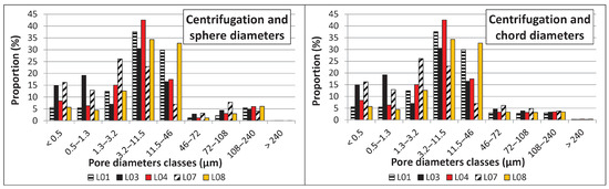
Figure 11.
Pore diameters distributions from laboratory and XRMT calculations for Lexos rock type. Distribution from centrifugation and sphere diameters analysis is displayed on the left, while distribution from centrifugation and chord lengths analyses is shown on the right.
4. Discussion
4.1. Validation of Calculated Parameters
Samples studied are all carbonate rocks divided in three different rock types: chalk, limestone, and dolomite. Although some differences have been demonstrated the previous part, each rock type has its specific properties. Nevertheless, the 30 samples have petrophysical characteristics consistent with carbonate rocks. Concerning structural properties, cementation indexes are usually between 1.8 and 4 for carbonate rocks [4] and more precisely between 2 and 2.2 for grainstone carbonates, with an increase of m in low-connected samples [31]. For samples with porosity comprised between 20 and 40% (such as Normandie), permeability is usually comprised between 1 and 10,000 mD [10], F should be between 6 and 125 (Equation (5)) while between 1.6 and 5 (Equation (6)), with the highest F and for and the lowest for [47,48]. For porosities between 10 and 20% (as Euville and Lexos), permeability is from 0.01 to 1000 mD [10], F and are higher and could reach respectively 100 and 3.1 for , while 1000 and 10 for . This is the case for our 30 samples (Table 1).
Given this consistence with literature data, we compared our dataset with other studies.
4.2. Influence of Rock Structure on Elastic Properties
Previously, we have seen that the microstructure of the rock affects the propagation of acoustic waves in samples. Porosity is the main parameter responsible for the variation of acoustic waves velocities. Indeed, velocities of P and S waves decrease when porosity increases [10]. Consequently, and from chalk are lower than limestone and dolomite ones, due to their lower porosities. Nevertheless, for a same porosity, very different and can occurred, which can be due to differences in pore structure [49]. Two equations relate to porosity through pore-fluid compressibility: WTA (Wyllie’s Time Average) [50] and RHG (Raymer-Hunt-Gardner) [51]. Our samples are situated below both trends (Figure 12 left), similarly to the main values plotted in literature [6,26]. The latter stated that the total travel time of a wave in a medium has no physical reason to be the sum of the travel times in the individual components. The low values of are therefore mainly due to a high microporosity [27], which are observed in our data set.
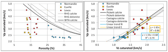
Figure 12.
Left: P-wave evolution with porosity. Right: P-wave evolution with S-wave evolution.
Moreover, and are related in a same equation with a positive correlation [52,53], where if one increases, the other follows (Figure 12 right). These equations fit the chalk and limestone samples, contrary to dolomite ones. Pickett’s equation stated for limestones, while our data set gives (with ) for Normandie and (with ) for Euville samples. The last one is therefore correlated with Pickett’s equation, while Normandie gives a remote result, probably due to its high proportion of small pores. However, Lexos samples present a significant number of variations due to the complexe structure of dolomite, and those two equations do not seem appropriate for our data.
Consequently, propagation of acoustic waves in rock seems to be strongly influenced by microstructure.
4.3. Influence of Rock Structure on Electrical Properties
Characterization of rock properties is partly related to permeability and electrical conductivity, which are related to geometry, pore connectivity and microstructure [6]. Indeed, the rock’s ability to let the fluid pass through is directly linked to rock structure. As seen before, electrical factors (, and ) are related to porosity, which induces a relation between porosity and permeability. A lot of relations between porosity and permeability have been carried out. Some connect the two by a n factor [15,16,54], while others take into account the grain diameter d in a non-fractal [15,16,22,55,56] and in a fractal dimension [57,58], the critical pore size [23,24], or the specific surface with the Kozeny factor c [27,59,60,61]. All these relations have been tested on our data set, and the results are summarized in Table 4.
Table 4.
Summary of permeability results calculated from literature.
Firstly, in line 1of Table 4, good correlations are given with the general law [15,16], consistent with laboratory measurements (Table 1). In line 2, adding critical porosity and fixing [54] give similar permeabilities for chalks, while underestimate the ones for limestone (lower than 1 mD). Inserting calculated porosities and permeabilities from Table 1 in line 3 [15,16] give grains diameters values d consistent with the ones measured and observed in Figure 1. Using these grain diameters d, various n factors are tested using the equation in line 4 [22] and higher permeabilities have been found. Similar values have been calculated using critical pore size , extracted from centrifugation (line 5) [24]. In contrast, as it has been carried out using equation in line 6 [23], taking into account formation factor F instead of porosity makes permeabilities significantly decrease.
These equations enable us to average dolomite permeability. Based on observations in Figure 1, an average grain diameter of 30 μm can be stated for dolomite samples, which gives permeabilities between 15 and 50 mD (line 3) [15,16], while lower with line 4 equation [22] and fixed. A critical pore size of 11.5 μm gives opposite permeabilities when taking into account porosity (line 5 equation [24]) or formation factor (line 6 equation [23]). Based on results obtained for limestone, dolomite is more likely to have low permeability.
Applying these different relationships to our data enable us to take into account the critical pore size with porosity (equation in line 5 from Table 4) [24] but gives overestimated permeability. On one hand, including grains diameter or critical pore size in permeability calculations is relevant. On the other hand, calculated permeabilities using formation factor are more consistent with measured data (Table 1). Consequently, transport properties in carbonate rocks seem to be mainly correlated with the rock structure, in particular the grain diameter.
However, adding a fractal dimension seems tricky for carbonate rocks because of the importance of microstructure, at the contrary of sandstones [57] and vesicular rocks [58]. Additionally, the specific surface, which can be compared to the poral surface accessible by the fluid, and by extension to our [27], does not seem correlated with porosity and permeability for our data set [27,59,60,61]. These failed correlations support the idea that microstructure plays a very important role. Indeed, is calculated from tomography images with a pixel resolution of 12 μm, which seems too large and inappropriate in transport properties determination.
4.4. Upscalling from Sample Measurements to Field Scale
Data from two large scale experimental sites are compared with our pore-scale data. On one hand, well loggings have been conducted on boreholes in Majorca chalks [9] to measure P waves velocities , resistivity of the reservoir and water that have been used to deduce formation factor F. Additionally, porosity has been measured on small cores extracted from these boreholes, with the same method as us. On the other hand, two sinkholes are used as boreholes on either side of a tunnel, dug inside detrital limestone on the Causse du Larzac [62,63]. P waves velocities , rock resistivity, density and water saturation have been measured. Formation factor F has been deduced from resistivity and porosity from density and water saturation. These three properties enable us to partly characterize the two reservoirs.
The evolution of formation factor F, porosity and P waves velocities with depth in Majorca illustrate that formation factor F and P waves velocities increase with decreasing porosity. This has also been observed on our pore-scale data, following well-known trends previously mentioned [46]. Then, large-scale properties compared with our dataset present some similarities and disparities (Figure 13). For a similar porosity, formation factors are on the same order of magnitude with very similar values. Data from Majorca experimental site are similar to Normandie data, which are both chalks; while Larzac data are similar to Euville data, which are both detrital limestones. However, for similar porosity, from chalk are higher for large-scale measurements than for laboratory ones, and are then closer to the RHG and WTA curves [50,51]. For detrital limestones, the same values of occur for lower porosity.
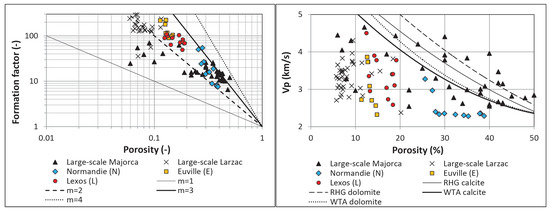
Figure 13.
On the left: evolution of formation factor depending on porosity; On the right: evolution of P waves velocities depending on porosity (modified from [9,63]).
Consequently, electrical properties and calculations seem to be applicable to each scale. However, even if measurements at large-scale are in the same order of magnitude than at pore-scale, and follow the known trends [46], correlations are not optimal. Acoustic measurements being usually correlated with microporosity proportion [27], disparities in measurements are explained by the difficulty of taking into account microporosity at large-scale. This validates the importance of pore-scale study.
5. Conclusions
In this study, we try to understand which parameters control large scale hydropetrophysical properties of carbonate reservoirs. For this purpose, plug samples of three rock types have been characterized from pore to core scale, with laboratory and imaging techniques. Samples petrophysical properties have then been compared with same parameters from large scale studies. Similar results in the same orders of magnitude were found.
Nevertheless, we highlight that microstructure is the most essential parameter in carbonates rocks characterization. Indeed, micropores control rocks properties. A change in their quantity and shape is responsible for considerable changes in petrophysical properties. For example, in samples with a low proportion of micropores, acoustic wave velocities are more likely to be high, inducing quite cohesive rocks. Similarities found with large scale reservoirs enable us to say that all scales are controlled by the same properties, inducing that microstructure study is essential in reservoir characterization.
Author Contributions
Conceptualization, M.L. and L.L.; methodology, M.L. and L.L.; validation, M.L. and L.L.; formal analysis, M.L.; investigation, M.L.; resources, L.L.; writing—original draft preparation, M.L.; writing—review and editing, L.L.; visualization, M.L.; supervision, L.L.; project administration, L.L.; funding acquisition, L.L. Both authors have read and agreed to the published version of the manuscript.
Funding
This research was funded by two projects: EC2CO (INSU-CNRS) StarTrek project and the JPI-Water UrbanWat project from WaterWorks2017; and by a CIFRE PhD fellowship provided by Voxaya and ANRT.
Institutional Review Board Statement
Not applicable.
Informed Consent Statement
Not applicable.
Data Availability Statement
Not applicable.
Acknowledgments
We acknowledge the MRI platform member of the national infrastructure France-BioImaging supported by the French National Research Agency (ANR-10-INBS-04, «Investments for the future»), the labex CEMEB (ANR-10-LABX-0004) and NUMEV (ANR-10-LABX-0020). We also acknowledge the petrophysics plateform members of Geosciences Montpellier Laboratory. We would like to acknowledge the 4 anonymous reviewers for their comments that allow improving the final version of this article.
Conflicts of Interest
The authors declare no conflict of interest.
Abbreviations
The following abbreviations are used in this manuscript:
| N | Normandie |
| E | Euville |
| L | Lexos |
| XRD | X-ray Diffraction |
| SEM | Scanning Electron Microscopy |
| XRMT | X-ray Micro-Tomography |
| XRCT | X-ray Computed Tomography |
| PV | Percolating Volume |
| REV | Representative Elementary Volume |
| RHG | Raymer-Hunt-Gardner |
| WTA | Wyllie’s Time Average |
References
- Chilingarian, G.V.; Mazzullo, S.J.; Rieke, H.H. Carbonate Reservoir Characterization: A Geologic-Engineering Analysis; Number 30, 44 in Developments in Petroleum Science; Elsevier: Amsterdam, The Netherlands; New York, NY, USA, 1992. [Google Scholar]
- Moore, C.H.; Wade, W.J. Carbonate Reservoirs: Porosity and Diagenesis in a Sequence Stratigraphic Framework, 2nd ed.; Number 67 in Developments in Sedimentology; Elsevier: Amsterdam, The Netherlands, 2013. [Google Scholar]
- Choquette, P.W.; Pray, L.C. Geologic Nomenclature and Classification of Porosity in Sedimentary Carbonates. Bulletin 1970, 54. [Google Scholar] [CrossRef]
- Lucia, F.J. Petrophysical parameters estimated from visual descriptions of carbonate rocks. J. Pet. Technol. 1983, 35, 629–637. [Google Scholar] [CrossRef]
- Lønøy, A. Making sense of carbonate pore systems. Bulletin 2006, 90, 1381–1405. [Google Scholar] [CrossRef]
- Regnet, J.; David, C.; Robion, P.; Menéndez, B. Microstructures and physical properties in carbonate rocks: A comprehensive review. Mar. Pet. Geol. 2019, 103, 366–376. [Google Scholar] [CrossRef]
- Eberli, G.P.; Baechle, G.T.; Anselmetti, F.S.; Incze, M.L. Factors controlling elastic properties in carbonate sediments and rocks. Lead. Edge 2003, 22, 654–660. [Google Scholar] [CrossRef]
- Verwer, K.; Eberli, G.P.; Weger, R.J. Effect of pore structure on electrical resistivity in carbonates. AAPG Bull. 2011, 95, 175–190. [Google Scholar] [CrossRef]
- Garing, C.; Luquot, L.; Pezard, P.A.; Gouze, P. Electrical and flow properties of highly heterogeneous carbonate rocks. Bulletin 2014, 98, 49–66. [Google Scholar] [CrossRef]
- Mavko, G.; Mukerji, T.; Dvorkin, J. The Rock Physics Handbook, 3rd ed.; Cambridge University Press: Cambridge, UK, 2020. [Google Scholar] [CrossRef]
- Dunham, R.J. Classification of Carbonate Rocks According to Depositional Textures; AAPG Special Volumes; AAPG: Tulsa, OK, USA, 1962. [Google Scholar]
- Lucia, F.J. Carbonate Reservoir Characterization: An Integrated Approach, 2nd ed.; Springer: Berlin, Germany; New York, NY, USA, 2007. [Google Scholar]
- Glover, P. What is the cementation exponent? A new interpretation. Lead. Edge 2009, 28, 82–85. [Google Scholar] [CrossRef]
- Archie, G. The Electrical Resistivity Log as an Aid in Determining Some Reservoir Characteristics. Trans. AIME 1942, 146, 54–62. [Google Scholar] [CrossRef]
- Kozeny, J. Uber kapillare Leitung des Wassers im Boden. Sitzungberichte Akadamie Wiss. Wien Abt. Ila 1927, 136, 271–301. [Google Scholar]
- Carman, P.C. Fluid Flow through Granular Beds. Trans. Inst. Chem. Eng. 1937, 15, 150–166. [Google Scholar] [CrossRef]
- Wyllie, M.R.J.; Rose, W.D. Application of the Kozeny Equation to Consolidated Porous Media. Nature 1950, 165, 972. [Google Scholar] [CrossRef]
- Cornell, D.; Katz, D.L. Flow of gases through consolidated porous media. Ind. Eng. Chem. 1953, 45, 2145–2152. [Google Scholar] [CrossRef]
- Clennell, M.B. Tortuosity: A guide through the maze. Geol. Soc. Lond. Spec. Publ. 1997, 122, 299–344. [Google Scholar] [CrossRef]
- Holzer, L.; Wiedenmann, D.; Münch, B.; Keller, L.; Prestat, M.; Gasser, P.; Robertson, I.; Grobéty, B. The influence of constrictivity on the effective transport properties of porous layers in electrolysis and fuel cells. J. Mater. Sci. 2013, 48, 2934–2952. [Google Scholar] [CrossRef]
- Rembert, F.; Jougnot, D.; Guarracino, L. A fractal model for the electrical conductivity of water-saturated porous media during mineral precipitation-dissolution processes. Adv. Water Resour. 2020, 145, 103742. [Google Scholar] [CrossRef]
- Bourbie, T.; Coussy, O.; Zinszner, B. Acoustics of Porous Media; Gulf Publishing Company: Houston, TX, USA, 1987. [Google Scholar]
- Thompson, A.; Katz, A.; Krohn, C. The microgeometry and transport properties of sedimentary rock. Adv. Phys. 1987, 36, 625–694. [Google Scholar] [CrossRef]
- Gueguen, Y.; Dienes, J. Transport properties of rocks from statistics and percolation. Math. Geol. 1989, 21, 1–13. [Google Scholar] [CrossRef]
- Anselmetti, F.S.; Eberli, G.P. The Velocity-Deviation Log: A tool to predict pore type and permeability trends in carbonate drill holes from sonic and porosity or density logs. AAPG Bull. 1999, 83, 450–466. [Google Scholar]
- Verwer, K.; Braaksma, H.; Kenter, J.A. Acoustic properties of carbonates: Effects of rock texture and implications for fluid substitution. Geophysics 2008, 73, B51–B65. [Google Scholar] [CrossRef]
- Weger, R.J.; Eberli, G.P.; Baechle, G.T.; Massaferro, J.L.; Sun, Y.F. Quantification of pore structure and its effect on sonic velocity and permeability in carbonates. Bulletin 2009, 93, 1297–1317. [Google Scholar] [CrossRef]
- Regnet, J.B.; Robion, P.; David, C.; Fortin, J.; Brigaud, B.; Yven, B. Acoustic and reservoir properties of microporous carbonate rocks: Implication of micrite particle size and morphology. J. Geophys. Res. Solid Earth 2015, 120, 790–811. [Google Scholar] [CrossRef]
- Japsen, P.; Bruun, A.; Fabricius, I.L.; Rasmussen, R.; Vejbæk, O.V.; Pedersen, J.M.; Mavko, G.; Mogensen, C.; Høier, C. Influence of porosity and pore fluid on acoustic properties of chalk: AVO response from oil, South Arne Field, North Sea. Pet. Geosci. 2004, 10, 319–330. [Google Scholar] [CrossRef]
- Le Ravalec, M.; Darot, M.; Reuschlé, T.; Guéguen, Y. Transport properties and microstructural characteristics of a thermally cracked mylonite. Pure Appl. Geophys. 1996, 146, 207–227. [Google Scholar] [CrossRef]
- Ramakrishnan, T.S.; Rabaute, A.; Fordham, R.J.; Ramamoorthy, R.; Herron, M.; Matteson, A.; Raghurman, B. A petrophysical and petrographic study of carbonate cores from the Thamama Formation. In Proceedings of the Abu Dhabi International Petroleum Exhibition and Conference, Abu Dhabi, United Arab Emirates, 11–14 November 1998. [Google Scholar] [CrossRef]
- Hebert, V.; Garing, C.; Luquot, L.; Pezard, P.A.; Gouze, P. Multi-scale X-ray tomography analysis of carbonate porosity. Geol. Soc. Lond. Spec. Publ. 2015, 406, 61–79. [Google Scholar] [CrossRef]
- Luquot, L.; Hebert, V.; Rodriguez, O. Calculating structural and geometrical parameters by laboratory measurements and X-ray microtomography: A comparative study applied to a limestone sample before and after a dissolution experiment. Solid Earth 2016, 7, 441–456. [Google Scholar] [CrossRef]
- Luquot, L.; Rodriguez, O.; Gouze, P. Experimental Characterization of Porosity Structure and Transport Property Changes in Limestone Undergoing Different Dissolution Regimes. Transp. Porous Med. 2014, 101, 507–532. [Google Scholar] [CrossRef]
- Rötting, T.S.; Luquot, L.; Carrera, J.; Casalinuovo, D.J. Changes in porosity, permeability, water retention curve and reactive surface area during carbonate rock dissolution. Chem. Geol. 2015, 403, 86–98. [Google Scholar] [CrossRef]
- Torquato, S.; Lu, B. Chord-Length Distribution Function for Two-Phase Random Media. Phys. Rev. E 1993, 47, 2950. [Google Scholar] [CrossRef] [PubMed]
- Gouze, P.; Luquot, L. X-ray microtomography characterization of porosity, permeability and reactive surface changes during dissolution. J. Contam. Hydrol. 2011, 120–121, 45–55. [Google Scholar] [CrossRef] [PubMed]
- Biot, M.A. Theory of Propagation of Elastic Waves in a Fluid-Saturated Porous Solid. II. Higher Frequency Range. J. Acoust. Soc. Am. 1956, 28, 179–191. [Google Scholar] [CrossRef]
- Gassmann, F. Elastic waves through a packing of spheres. Geophysics 1951, 16, 673–685. [Google Scholar] [CrossRef]
- Waxman, M.; Smits, L. Electrical conductivities in oil-bearing shaly sands. Soc. Pet. Eng. J. 1968, 8, 107–122. [Google Scholar] [CrossRef]
- Reatto, A.; Da Silva, E.M.; Bruand, A.; Souza Martins, E.; Lima, J.E.F.W. Validity of the Centrifuge Method for Determining the Water Retention Properties of Tropical Soils. Soil Sci. Soc. Am. J. 2008, 72, 1547–1553. [Google Scholar] [CrossRef]
- Espinoza, D.N.; Santamarina, J.C. Water-CO2-mineral systems: Interfacial tension, contact angle, and diffusion - Implications to CO2 geological storage. Water Resour. Res. 2010, 46. [Google Scholar] [CrossRef]
- Gouze, P.; Melean, Y.; Le Borgne, T.; Dentz, M.; Carrera, J. Non-Fickian dispersion in porous media explained by heterogeneous microscale matrix diffusion. Water Resour. Res. 2008, 44. [Google Scholar] [CrossRef]
- Ghanbarian, B.; Hunt, A.G.; Ewing, R.P.; Sahimi, M. Tortuosity in Porous Media: A Critical Review. Soil Sci. Soc. Am. J. 2013, 77, 1461–1477. [Google Scholar] [CrossRef]
- Tanikawa, W.; Shimamoto, T. Klinkenberg effect for gas permeability and its comparison to water permeability for porous sedimentary rocks. Hydrol. Earth Syst. Sci. Discuss. 2006, 3, 1315–1338. [Google Scholar] [CrossRef]
- Mavko, G.; Mukerji, T.; Dvorkin, J. The Rock Physics Handbook: Tools for Seismic Analysis of Porous Media, 2nd ed.; Cambridge University Press: Cambridge, UK; New York, NY, USA, 2009; OCLC: ocn268793772. [Google Scholar]
- Casteleyn, L.; Robion, P.; Collin, P.Y.; Menéndez, B.; David, C.; Desaubliaux, G.; Fernandes, N.; Dreux, R.; Badiner, G.; Brosse, E.; et al. Interrelations of the petrophysical, sedimentological and microstructural properties of the Oolithe Blanche Formation (Bathonian, saline aquifer of the Paris Basin). Sediment. Geol. 2010, 230, 123–138. [Google Scholar] [CrossRef]
- Casteleyn, L.; Robion, P.; David, C.; Collin, P.Y.; Menéndez, B.; Fernandes, N.; Desaubliaux, G.; Rigollet, C. An integrated study of the petrophysical properties of carbonate rocks from the “Oolithe Blanche” formation in the Paris Basin. Tectonophysics 2011, 503, 18–33. [Google Scholar] [CrossRef]
- Anselmetti, F.S.; Eberli, G.P. Controls on sonic velocity in carbonates. Pure Appl. Geophys. 1993, 141, 287–323. [Google Scholar] [CrossRef]
- Wyllie, M.R.J.; Gregory, A.R.; Gardner, L.W. Elastic wave veloticies in heterogeneous and porous media. Geophysics 1956, 21, 41–70. [Google Scholar] [CrossRef]
- Raymer, L.; Hunt, E.; Gardner, J.S. An Improved Sonic Transit Time-To-Porosity Transform. In Proceedings of the SPWLA 21st Annual Logging Symposium, Lafayette, Louisiana, 8–11 July 1980. [Google Scholar]
- Pickett, G. Acoustic Character Logs and Their Applications in Formation Evaluation. J. Pet. Technol. 1963, 15, 659–667. [Google Scholar] [CrossRef]
- Castagna, J.P.; Backus, M.M. (Eds.) Offset-Dependent Reflectivity—Theory and Practice of AVO Analysis; Society of Exploration Geophysicists: Houston, TX, USA, 1993. [Google Scholar] [CrossRef]
- Martys, N.S.; Torquato, S.; Bentz, D.P. Universal scaling of fluid permeability for sphere packings. Phys. Rev. E 1994, 50, 403–408. [Google Scholar] [CrossRef]
- Carman, P.C. Some physical aspects of water flow in porous media. Discuss. Faraday Soc. 1948, 3, 72–77. [Google Scholar] [CrossRef]
- Carman, P.C. Flow of Gases through Porous Media; Academic: Cambridge, MA, USA, 1956. [Google Scholar]
- Pape, H.; Clauser, C.; Iffland, J. Permeability prediction based on fractal pore-space geometry. Geophysics 1999, 64, 1447–1460. [Google Scholar] [CrossRef]
- Costa, A. Permeability-porosity relationship: A reexamination of the Kozeny-Carman equation based on a fractal pore-space geometry assumption. Geophys. Res. Lett. 2006, 33, L02318. [Google Scholar] [CrossRef]
- Paterson, M. The equivalent channel model for permeability and resistivity in fluid-saturated rock—A re-appraisal. Mech. Mater. 1983, 2, 345–352. [Google Scholar] [CrossRef]
- Walsh, J.B.; Brace, W.F. The effect of pressure on porosity and the transport properties of rock. J. Geophys. Res. Solid Earth 1984, 89, 9425–9431. [Google Scholar] [CrossRef]
- Fabricius, I.L.; Baechle, G.; Eberli, G.P.; Weger, R. Estimating permeability of carbonate rocks from porosity and vp/vs. Geophysics 2007, 72, E185–E191. [Google Scholar] [CrossRef]
- Fores, B. Gravimetry and Ambient Seismic Noise Monitoring for Hydrological Modeling: Application to the Durzon Karstic Basin (Larzac, France). Ph.D. Thesis, Université Montpellier, Montpellier, France, 2016. [Google Scholar]
- Fores, B.; Champollion, C.; Lesparre, N.; Pasquet, S.; Martin, A.; Nguyen, F. Variability of the water stock dynamics in karst: Insights from surface-to-tunnel geophysics. Hydrogeol. J. in press.
Publisher’s Note: MDPI stays neutral with regard to jurisdictional claims in published maps and institutional affiliations. |
© 2021 by the authors. Licensee MDPI, Basel, Switzerland. This article is an open access article distributed under the terms and conditions of the Creative Commons Attribution (CC BY) license (https://creativecommons.org/licenses/by/4.0/).