Article

Detecting Change between Urban Road Environments along a Route Based on Static Road Object Occurrences

by
Zoltán Fazekas
1,2,*,
László Gerencsér
1 and
Péter Gáspár
1
1
Institute for Computer Science and Control (SZTAKI), Eötvös Loránd Research Network (ELKH), 13-17. Kende Utca, H-1111 Budapest, Hungary
2
Department of Control for Transportation and Vehicle Systems, Faculty of Transportation Engineering and Vehicle Engineering, Budapest University of Technology and Economics (BME), 2 Stoczek Utca, H-1111 Budapest, Hungary
*
Author to whom correspondence should be addressed.
Appl. Sci. 2021, 11(8), 3666; https://doi.org/10.3390/app11083666
Submission received: 24 March 2021 / Revised: 10 April 2021 / Accepted: 14 April 2021 / Published: 19 April 2021
(This article belongs to the Section Robotics and Automation)

Abstract

:

Featured Application

A road environment-type (RET) detection function could improve the road awareness of inexperienced car drivers, especially in urban areas, and by doing so, it could slightly raise the urban traffic safety. A pragmatic implementation could make use of static road object data, e.g., traffic sign (TS) data, that is already collected and available on-board. It could rely on the TS recognition function offered by advanced driver assistance systems (ADAS). Furthermore, apart from its primary function, the RET detection system could provide reciprocal information—with respect to the current RET—for various ADAS and autonomous driving (AD) computations and subsystems. Making use of such reciprocal information could speed up the ADAS/AD computations, and render their results more accurate and more reliable, e.g., via introducing parameter constraints and marking regions-of-interest.

Abstract

For over a decade, urban road environment detection has been a target of intensive research. The topic is relevant for the design and implementation of advanced driver assistance systems. Typically, embedded systems are deployed in these for the operation. The environments can be categorized into road environment-types. Abrupt transitions between these pose a traffic safety risk. Road environment-type transitions along a route manifest themselves also in changes in the distribution of traffic signs and other road objects. Can the placement and the detection of traffic signs be modelled jointly with an easy-to-handle stochastic point process, e.g., an inhomogeneous marked Poisson process? Does this model lend itself for real-time application, e.g., via analysis of a log generated by a traffic sign detection and recognition system? How can the chosen change detector help in mitigating the traffic safety risk? A change detection method frequently used for Poisson processes is the cumulative sum (CUSUM) method. Herein, this method is tailored to the specific stochastic model and tested on realistic logs. The use of several change detectors is also considered. Results indicate that a traffic sign-based road environment-type change detection is feasible, though it is not suitable for an immediate intervention.

1. Introduction

Despite of the on-going research on self-explaining road layouts and designs [1,2], and on the computerized recognition methods of such designs and layouts, e.g., on methods that apply artificial intelligence methodology [3], setting up traffic signs (TSs) along the roads and traffic lights in road junctions and near pedestrian crossings by the transport authorities still remains a customary measure for reducing traffic safety risks in urban areas [4]. Clearly, there are other viable alternative measures, as well as supplementary ones for the purpose. These include—among many others—the installation of speed reduction markings onto the road-surface [5] and the installation of vehicle- to-infrastructure (V2I) communication facilities, e.g., to succor the TS recognition (TSR) function offered by advanced driver assistance systems (ADAS) [6] and self-driving cars [7]. In a wider sense, V2I communication succors the road, traffic and vehicle data gathering, fusion, and dissemination, and through these data processes, it is expected to have a significant beneficial impact on traffic safety [8]. More specifically, V2I communication can be used for raising the road-awareness of car-drivers, as well as that of the intelligent and the self-driving road vehicles. Furthermore, it can be used for providing the human drivers and the smart vehicular systems with current traffic information with respect to the region, town, and area, on the one hand, and with some very specific dynamic information on individual vehicles in the vicinity, on the other [9].
When speaking about raising road awareness of drivers, one is obliged to speak about the Global Navigation Satellite System (GNSS), a system that is used by masses of people around the world. According to [10], the GNSS devices per capita averaged out at 0.8 across the countries of world in 2019. The GNSS is used with wide variety of devices running map-based applications, a significant percentage of these devices are installed on-board cars. The brief history of the navigational systems and their respective precisions are presented in [11]. The paper provides a fresh outlook on the navigational needs of and the available navigational solutions for autonomous vehicles and systems. As it often happens to popular services, devices, and applications, threats against these surface from time to time. Such threats have surfaced also against the GNSS service [12]. Although the number of successful navigational spoofing attacks is still negligible, the navigational signal deteriorations due to other—i.e., non-hostile—factors are clearly not. For instance, the signal reception is often brought down, or even blocked by the high-rise buildings in densely built urban areas. Some examples in this context are presented in [13].
The speed reduction measures implemented in urban areas are motivated by the traffic safety concerns associated with the intense road traffic and the limited space available there for the driving maneuvers [14]. While driving, and particularly while driving in urban areas, drivers need to perform numerous mental and control tasks—ranging from those associated with limb-movement to those required for complex driving maneuver planning and execution—within stringent time and spatial constraints and with high reliability [15]. Furthermore, these tasks must be performed in presence of disturbances, such as unfavorable lighting, adverse weather, and traffic conditions [16]. In addition, the older age of the driver may contribute to the perceived difficulty of these tasks [17].
A system, which pays attention to the driver’s activity within the car and also to aspects of the urban road environment, was developed as part of the Urban Intelligent Assist Research Initiative some years ago [18], and since then, other systems with similar, or enhanced capabilities followed suit [19,20]. The effect of driving experience on drivers’ adaptation to road environment complexity—a notion closely related to that of the road environment type (RET) used herein—in urban areas was investigated in a simulation study [21]. The findings of the study underline the need for an automatic RET detection function, and indicate that such a function is particularly useful for car-drivers lacking prolonged driving experience, and also for older drivers.
Several algorithmic approaches and sensor arrangements were devised, applied, and tested for detecting, characterizing, and categorizing urban road environments based on image and/or point cloud data [22,23,24]. In the application considered herein, the urban road environment appears around and sweeps past an ego-car while it is driven in an urban area. The data streams used for the purpose of road environment detection and analysis originate—among others—from one or more camera and one or more light detection and ranging (LiDAR) sensor. In a viable implementation of a road environment detection and classification system that is capable of assisting a car driver while driving, either a comprehensive real-time on-board processing of the respective raw data streams is required (direct processing) or a timely access to and further processing of the data—rendered by some other real-time application/subsystem on-board—on certain distinguishing road objects (ROs) are necessary (indirect processing).
In the above cited papers, the real-time requirements were limited to data synchronization and data collection issues, while the bulk of the processing, e.g., simultaneous localization and mapping (SLAM), and object segmentation, were carried out in a post-processing manner. Nevertheless, a large portion of the processing presented in these papers is real time capable and could be used in direct implementations.
The approach presented in [22] builds and then segments the point cloud originating from a ground-level LiDAR device moving along a given trajectory. The aim of the authors was to produce editable—simplified, but visually still pleasing—object-models that lend themselves for fast visualization. The target areas were the residential urban areas in the United States. These areas are characterized by their low-rise buildings without strong and extensive repetitive patterns. The semantical labeling and various analysis steps follow the mentioned preprocessing steps. Simple models of the individual houses in the area are then created. The basic building blocks of the models are simple, symmetric, and convex geometric blocks. These blocks—together with their spatial arrangement and their connection graph—form an easy-to-handle geometric model of the individual buildings. By aggregating the certain features of the individual buildings for an area (e.g., by computing the average building dimensions and the average distance between nearest buildings), the residential urban road environment can be adequately characterized.
The system presented in [23] extracts the characteristics of individual buildings rather than those of more extensive road environments. Nonetheless, the building characteristics, such as building height and building complexity—again aggregated for a given area, or along a route—together with the spatial densities of the buildings there, are definitive in the respect of the RET.
A multi-sensor and multi-precision data collection campaign is described in [24]. It was a car-based campaign that made use of an array of different environment perception, navigational, and motion sensors. These included four LiDARs, a pair of stereo cameras, a fiber optics gyroscope and encoder sensors for the tires. The data collection trips covered diverse complex urban environments in Korea, with a clear emphasis on those environments, where GPS reception is highly unreliable. The collected data were organized into a publicly accessible dataset that includes the measured ego-car trajectories, the raw and processed point cloud data from the LiDAR sensors, as well as the ego-car trajectories with improved precision computed via SLAM.
Other approaches, e.g., the ones presented in [25,26], rely object-level data as inputs to the urban RET detection function, i.e., they follow an indirect processing approach. In a feasible realization, the raw data streams originate from the very same sensors as in the direct case, but the respective data streams reach the RET detection subsystem only after having been processed and considerably compressed by one or more ADAS subsystem. The resulting data are an object-level description of the road environment, i.e., an RO log. This log serves as an input to the indirect RET detection function.
The on-board data processing described above, as well as other road, traffic, and vehicular data processing carried out in various ADAS subsystems (e.g., lane detection, TSR, detection of nearby vehicles) can also be looked at from, analyzed with respect to, and formulated using a static reference point. Setting up and using a local dynamic map (LDM) [27] could serve these purposes, and provide additional conceptual support for the developers of ADAS functions. LDM is a widely used model for representing, and a standardized technology for integrating static, temporary, and dynamic road, traffic, and vehicular information into a static geographical context by means of a common coordinate reference. Customarily, it has four object layers describing and managing ROs that are subject to change and exhibit dynamics at different time scales. More concretely, these layers store and handle data on permanent static, transient static, transient dynamic, and highly dynamic ROs, respectively. For instance, when framing the static RO-based urban RET detection task in LDM, the ego-car is seen as a highly dynamic RO. A crossroads (CRs) intersection of streets is a permanent static RO in this model. The intersection can be associated with other ROs (e.g., with fixed traffic lights located there, which are transient static ROs). The lanes, lane markings, pedestrian crossings, and the conventional TSs are transient static ROs, while the TSs displayed by variable message sign boards can be classified as transient dynamic ROs. The RETs can be treated as permanent static features of an area or of a sub-network of roads.
One could look at the ROs in an urban settlement and collect and compile their location and categorical data into a map layer, e.g., in the way data contributors of OpenStreetMap maps do with roads, railways, rivers, and various locations of importance [28]. By selecting appropriate subsets of TSs—i.e., TS subsets that are characteristic to certain RETs—various sublayers of the RO layer can be created, displayed, and analyzed. The analysis could include a Delaunay triangulation of the TS locations within a sublayer, and then one could look for dense clusters of triangles in the generated structure. By carrying out similar processing for a number of sublayers, a TS-based RET categorization of the urban area can be created.
By further processing the map-based representation of TSs and other ROs, one could derive other interesting sublayers that relate to seasonal, weekly, or daily validity of the TSs and could derive a sublayer representing weather-related TSs (e.g., TSs applicable for wet, snowy and icy road conditions). For instance, the sublayer representing the within-the-day validity of TSs—indicated by auxiliary signs or time intervals attached to the TSs—should reflect the daily dynamics of traffic source and sink structure of the area [29]. Clearly, the mentioned dynamics are closely related to the RET categorization used herein.
In our view, such sublayers—compiled, e.g., from data gathered in car-based data collection campaigns—could give useful hints to road authorities and administration as to where to place additional TSs and auxiliary signs or remove unnecessary existing ones. Herein, however, we stick to the route-based sampling of the TSs of the urban area, the map-based processing touched upon above will be addressed in further research.
In [25,26], the urban road environments were categorized into three RETs, namely, into downtown (Dt), residential (Res), and industrial/commercial (Ind) areas. The ROs represented in the object-log were the TSs and CRs encountered along the route. In an advantageous implementation foreseen, both the TS and the CR data originate from their respective dedicated ADAS subsystems. While in case of the TS data, the corresponding subsystem, i.e., the TSR ADAS subsystem, is quite common in recent production cars, the CR detection ADAS function is fairly uncommon at this point of time. It is expected though that in the coming years, the LiDAR sensors developed for automotive applications will pave the way for the spread of such an ADAS subsystem.
A good insight in ADAS system architectures, various ADAS subsystems and functions, as well as the respective methods and computations involved is given in [30]. A survey on TSR methods and systems is given in [31], while in [32], a mapping and navigation system developed for large-scale global positioning-denied sites is introduced. The system is capable of detecting CRs, intersections, and other road infrastructure.
The static RO-based urban RET detection approach proposed in [25], and some further approaches make use of a variety of classification and change detection (CD) methods known from the statistical inference literature. In the cited paper, it is presumed that the static ROs in general, and the considered TSs and the CRs, in particular, occur along the route according to an inhomogeneous discrete-variable binomial process. The minimum description length (MDL) methodology is then applied to detect and locate change in the character of the road environment sweeping past the ego-car.
The lane-keep assist ADAS and the lane following autonomous driving (AD) subsystems, which perforce continually identify the current and neighboring lanes, and estimate their widths, as well as the TSR ADAS and AD subsystems, which locate, identify, and track the TSs encountered by the ego-vehicle, are of particular interest in the context of RET detection. First, such ADAS subsystems are already available on-board many production cars, second, the categorical and spatial distribution of TSs, as well as, the lane-widths and the number of lanes—in the current cross-section of the road or in an aggregated form (e.g., average lane-width, average number of lanes)—carry information that can be useful in determining the RET of the given urban area.
It should be emphasized that a timely feedback of the RET information to the above ADAS and AD subsystems could increase their effective processing speed and lower the rate of misclassifications via setting practical parameter constraints for the computations involved. Such constraints could be of geometrical nature and could take the forms of Boolean, probabilistic, and fuzzy regions-of-interest (ROIs), respectively, e.g., within image frames of video sequences [33]. While in case of point clouds, volumes-of-interest, again meant in a Boolean, in a probabilistic, and in a fuzzy way, respectively, could be marked and used [34]. As a further application of such reciprocal information, the characteristic size range of TSs—for a given RET—could be used for validating the detected TS candidates [35].
Similar processing benefit could be gained from the above outlined information feedback in case of other presently not so wide-spread driver assistance functions, such as the CR detection. Furthermore, information on the current RET is also important for suggesting/choosing appropriate vehicle speed and acceleration/deceleration for the ego-car. An embedded testbed architecture for testing functions of self-driving cars was proposed in [36]. It could also facilitate the seamless integration of the static RO-based RET detection function into the intelligent vehicle control systems.
In the following, it will be assumed that TS occurrences are reliably detected and logged by the on-board TSR ADAS subsystem, moreover, this log is passed on to the RO-based—in the following practically TS-based—RET detection system in real-time.
It was our aim to choose, adapt, and validate a mathematically sound CD method that makes provision for and relies on a simple, but realistic stochastic model of the static RO placement and occurrences, in general, and of the TS placement and occurrences, in particular, for the purpose and in the context of detecting transitions between road environments of different character—or more concretely, between road environments of different RETs—in order to assist car drivers, human, and robotic drivers alike, in their driving tasks and activities. The continuous-time inhomogeneous marked Poisson process (IMPP) was identified as a possible stochastic model to work with.
It should be noted, however, that in real life, the static RO placements—including those of TSs and traffic lights—are governed by technical and administrative guidelines [37], from time to time they are subjects of potentially lengthy conciliatory procedures between locals and road administration. The final decisions are therefore taken at different administrative levels. Some aspects of this occasionally complicated process are outlined in [38]. As in [25,26] also herein, the occurrences are considered along routes. These routes are assumed to be random, but they are, in fact, based on intelligent choices made by the drivers.
Results gained via simulation implementing the IMPP model and making use of realistic data indicate that a TS-based RET CD is feasible and can be used for driver assistance, though it is not suitable for initiating an immediate intervention in critical situations. A more varied selection of static ROs—including, e.g., CRs, traffic lights, and pedestrian crossings—would further improve the feasibility of the RET CD. Similar utility and feasibility are expected for the RET detection and identification function computed with several RET change detectors and an artificial neural network (ANN) that merges and mushes together the detected RET transitions.

2. Materials and Methods

2.1. Car-Based Collection of Static Road Object Data from Various Urban Road Environments

A series of car-based static RO data collection trips was carried out in Hungary in 2017. The data were collected from a number of urban areas. Data concerning a richer set—than presented here—of TSs and of some more characteristic ROs was gathered. The TSs and other ROs were recorded manually along the routes—together with the RETs of the given areas—with the help of a dedicated tablet-based Android application, while the trajectory data of the trip was collected automatically by the app in every few seconds, and at the times of the TS and other RO entries [25].
The data collection personnel consisted of two persons: a driver and a data entry assistant. The manual data entry was made easy by the array-like screen design with TSs and RO symbols. In case of parametrized TSs, e.g., speed limits, the standard options (i.e., 10 km/h, 20 km/h, …, 70 km/h) were offered—also in pictorial form—after the general TS type. Specific symbols, i.e., touch-screen keys, were offered for entering the considered RETs, the repeated entries, for the cancelations of the last entry, and for entering verbal comments. The location, time, TS/RO, and RET categorical data were stored in a text-file in a comma separated values (cvs) format. After the trips, the csv files were stored as spreadsheets and were converted to various formats (e.g., kml) for post-processing and visualization.
From the above data collection, the relevant TS rates—along routes in the considered RET areas—were known. The empirical rates for the Applsci 11 03666 i001 (“No stopping” (NS)), Applsci 11 03666 i002, (“Parking lot” (PL)), Applsci 11 03666 i003 (“Give way” (GW)), and Applsci 11 03666 i004 (“Max speed 30 km/h” (SL)) TSs were used herein as a priori estimates of the reference rates for the marked Poisson processes. These rates are given in Table 1 for routes within Dt and within Res areas.

2.2. Mathematical Models and Methods

As it was mentioned in the Introduction, the continuous-time IMPP stochastic model had been chosen for characterizing the along-the-route placement and occurrence of TSs jointly for the purpose of RET CD in the present study. For a profound treatment of the mathematical theory of Poisson processes, see [39].
In the chosen stochastic approach, the TS data logs are seen as realizations of an IMPP. The CD method used commonly in conjunction with Poisson processes is the cumulative sum (CUSUM) method. Detailed expositions of such methods can be found in [40,41]. By assuming the validity of the IMPP model—at least with respect to the considered RETs and considered TSs—for describing and characterizing TS placements and occurrences along routes within and between urban environments, our task narrowed down to adapt a suitable CUSUM method for the purpose, and validate it with realistic TS data.
It was our intention to adopt and validate a continuous-time variant of the CUSUM method for CD. Furthermore, trade-off is sought between the false alarm rate and the expected detection lag associated with the TS sequences and to provide hints for choosing appropriate thresholds for the change detectors.
The continuous-variable variant of the CUSUM method for CD in IMPP realizations is derived in this subsection. The working of the RET change detectors implementing this method is demonstrated in Section 3.1 and Section 3.2. The change detectors presented therein have been tuned to detect two different RET transitions, namely, Dt to Res and Res to Dt transitions, and are tested with synthetic input sequences.

2.2.1. Modelling TS Occurrences within a Given Urban Road Environment

As a first step, we are going to model the TS placements, occurrences, and detections—along a random route and within a certain urban road environment—jointly as events of a continuous-variable homogeneous marked Poisson process (HMPP).
In the literature dealing with Poisson processes usually the mentioned continuous variable is the time. Although, with the notations used herein, as well as with the verbal expressions describing relations between values, we are going to comply with this “temporal” convention, and it should be emphasized that the path-length—that has been covered by the ego-car—is chosen to be the continuous spatial variable.
Let { T n , k n } , where k n { 1 , 2 , , K } and K , be a marked Poisson process with counting measures N k ( ) . These are defined as N k ( A ) = # { n : T n A } , where A is typically an interval. Let the rates associated with the marked Poisson process be λ k , assuming spatial—and particularly along-the-route—homogeneity, and let the corresponding reference rates of the Poisson process be λ k 0 . Then, the negative logarithm of the likelihood-ratio of an observation sequence ( { T n , k n } ) , T n < T is given by
D T N T k ( λ k λ k 0 ) k N k ( T ) log ( λ k λ k 0 )
where N k ( T ) is the number of events of type k prior to T .
Assuming now that λ 0 = { λ k 0 } is the true set of process parameters, furthermore assuming that λ = { λ k } is a set of tentative parameter values, and writing D T N = D T N ( λ ) , we have the following inequality:
E { D T N ( λ ) } 0 .
The left-hand side is simply the Kullback-Leibler (KL) divergence of the true distribution from the estimated one. Using the common notation of the KL divergence, the left-hand-side of the above inequality can be rewritten as
E { D T N ( λ ) } = D K L ( mPois ( λ 0 T ) mPois ( λ T ) ) ,
where mPois ( ) represents the distribution corresponding to the marked Poisson process, while D K L ( mPois ( λ 0 T ) mPois ( λ T ) ) is the expected number of extra nats—NB: not bits, but nats, as the natural logarithm is used in Equation (1), not log 2 —required to encode the observation sequence from the distribution mPois ( λ 0 T ) using a code optimized for the distribution mPois ( λ T ) rather than using the code optimized for mPois ( λ 0 T ) .
Associated with D T N ( λ ) is the computable quantity
L T ( λ ) T k λ k k N k ( T ) log ( λ k T )
L T ( λ ) can be interpreted as the approximate length of an optimal code encoding the observation sequence, were λ the true set of the process parameters. Considering, however, that L T ( λ ) is dependent on λ 0 —i.e., on the “real” true set of process parameters—via N k , we can write L T ( λ ) = L T ( λ 0 , λ ) , and similarly, we can indicate the same kind of dependency for D T N , i.e., D T N = D T N ( λ ) = D T N ( λ 0 , λ ) .

2.2.2. Modelling TS Occurrences in a Neighboring Urban Road Environment

In conjunction with a second road environment that borders the one looked at in the previous subsection, let us now consider another marked Poisson process with parameters μ 0 = { μ k 0 } . The probability distribution corresponding to this process is mPois ( μ 0 T ) . The counting measures M k ( ) are used for counting the events of different types, i.e., for counting the occurrences of the various TSs, separately.
Let the a priori estimate of μ 0 be μ . Then, similarly to our comments with respect to L T ( λ ) defined in Equation (4), the approximate length of an optimal code encoding the observation sequence observed within this second road environment—were μ the true set of the process parameters—is given in Equation (5)
J T ( μ ) T k μ k k M k ( T ) log ( μ k T ) .
Considering that J T ( μ ) is dependent on μ 0 —i.e., on the “real” true set of process parameters—through event counts M k , we can write J T ( μ ) = J T ( μ 0 , μ ) . Furthermore, the negative logarithm of the likelihood-ratio of an observation sequence—observed within this second road environment—can be written as D T M = D T M ( μ ) = D T M ( μ 0 , μ ) .

2.2.3. Modelling TS Occurrences over Two Neighboring Urban Road Environments

If λ and μ are reasonable estimates of λ 0 and μ 0 , respectively, then D T N ( λ 0 , λ ) and D T M ( μ 0 , μ ) are going to remain relatively small. We shall consider the case, when the parameter-sets of the two marked Poisson process differ considerably, i.e., λ 0 and μ 0 differ considerably with λ and λ 0 still being close to each other, and with μ and μ 0 still being close to each other. Then D T N ( λ 0 , μ ) and D T M ( μ 0 , λ ) are going to be large.
Furthermore, using the encoding argument outlined above, L T ( λ ) L T ( μ ) will have a tendency to decrease in time (i.e., with T ), and similarly, J T ( μ ) J T ( λ ) will also have such a tendency. The negated version of the latter, i.e., J T ( λ ) J T ( μ ) , on the other hand, will have a tendency to increase in time. More clearly, using the defining formulae in Equations (4) and (5), respectively,
L T ( λ ) L T ( μ ) = T k ( λ k μ k ) k N k ( T ) log ( λ k μ k )
tends to decrease with T , while
J T ( λ ) J T ( μ ) = T k ( λ k μ k ) k M k ( T ) log ( λ k μ k )
tends to increase with T .

2.2.4. Detecting Change between Urban Road Environments and Locating the Change Point

Assume now a switch from the first marked Poisson process to the second, i.e., from mPois ( λ 0 T ) to mPois ( μ 0 T ) , and accordingly a switch from respective counting measures N k ( ) to M k ( ) at time τ . Then for T τ
g T g T ( λ , μ ) L T ( λ ) L T ( μ )
tends to decrease with T . Let us now introduce the notation T * = T τ . For T > τ , i.e., for T * > 0 , g T is defined as follows
g T g T ( λ , μ ) g τ + J T * τ ( λ ) J T * τ ( μ ) ,
where J T * τ ( λ ) J T * τ ( μ ) is to be computed according to a modified version of Equation (7), as shown below
J T * τ ( λ ) J T * τ ( μ ) = T * k ( λ k μ k ) k M τ k ( T * + τ ) log ( λ k μ k )
here the counting measures M τ k ( ) count events in the same way as M k ( ) with the only difference that they now count events only from τ onwards.
For T > τ , g T tends to increase with T . To estimate the location τ , one should monitor function g T . Then, in order to determine τ , we need to wait for an increasing trend in g T to appear.
In order to find out whether a change in the stochastic model has occurred, or not, and if it has, when/where, one should compute the minimum of g T on-the-fly with a Page-Hinkley change detector (PHCD), see [42,43] for the detailed derivation of the change detector.
Using g T , the PHCD, h T is defined as
h T g T inf s T g s .
A change is thought to have occurred if h T exceeds a threshold δ > 0 . As it will be clear from the examples presented in Section 3.1 and Section 3.2, the choice of δ is crucial for the proper working of the detector.
It can be shown—following the line of thoughts presented in [44]—that under the hypothesis of no-change, h T is L-mixing, and the false alarm probability is exponentially decaying in δ : P ( h T δ ) C e a δ with some a > 0 . Hence the false alarm rate itself is exponentially decaying in δ . As a consequence, the false alarm rate can be effectively reduced by choosing larger δ . On the other hand, if δ is chosen to be too large, then the detection lag can be too long or even transitions can be missed.

2.2.5. Basic Properties of Functions g T and h T

Before getting on to elaborate concrete TS-based RET CD examples in Section 3.1 and Section 3.2, it is worthwhile to look more closely at the functions involved in the CD computations, namely, to g T and h T . The diagrams of these functions are composed of linear segments.
In case of g T , each of these linear segments has the same slope, and at either end of a segment, there can be a “jump”. The jump can be either an upward jump, or a downward jump depending on the particular event and on the process parameters.
In case of h T , the situation is slightly more complicated. Apart from the linear segments with the same slope, if any such segment remains in the diagram, there can be broken lines reaching the horizontal axis, and a number of linear segments along this axis. Furthermore, all the constituting linear segments and broken lines of h T are located in the upper half-plane that includes also the horizontal T axis.

3. Results

3.1. Examples

Let us now see two CD examples from the given application field. In these examples, we intend to detect change in the RET based on TS occurrences along a route. The full length of the trip represented in the table is 4.6 km. The TSs are assumed to be detected and located by an on-board TSR system.
The TS locations are marked with the corresponding TSs in the top band of Table 2. The sequence given there is synthetic, and has been compiled for the purpose of demonstrating
  • a RET transition from a Dt to a Res area (denoted by Dt → Res), if the virtual journey is taken from the left, and
  • a RET transition from a Res to a Dt area (denoted by Res → Dt), if the journey is taken from the right.
In the middle and the bottom bands of Table 2, the actual counts of the NS, PL, GW, and SL TSs for the virtual trips starting from the left, and from the right, respectively, are given. These counts have been produced in a unified and generic manner, i.e., without demarking the validity intervals of the respective counting measures.
As these counts are denoted simply by N N S , N P L , N G W , and N S L in the present and in the subsequent subsections, care should be taken to use them properly, i.e., according to the direction of the virtual trip.
In the sequence given in the top band, each “—” signifies a 0.2 km path-length along the route without any relevant TSs—facing the ego-car—installed/detected along the corresponding patch of road. It should be underlined that these fixed path-length route-segments are used in the examples simply for convenience, i.e., to make diagrammatic representation of the TS sequence, as well as the virtual trip easier to follow, and to make the calculations and diagrams easier to verify.
In each of the two examples that are presented in this subsection, the specific PHCD is applied to a RET transition that is homologous to the one, the PHCD has been tuned to.
First, let the ego-car start its virtual trip from the left. This case is described in detail in Example No. 1.

3.1.1. Example No. 1: A Dt → Res Change Detector Applied to a Homologous RET Transition

In the TS sequence given in the top band of Table 2, the intended RET transition (i.e., the Dt → Res) occurs at about the path-length of 2.2 km (i.e., having covered eleven dashes from the left in the band). The presence of such a RET transition in the synthetic sequence was secured by having inserted into it five TSs that are more characteristic of the Res areas than of the Dt areas—see the rightmost column of Table 1—in consecution and reasonably close to each other starting from this path-length along the virtual route.
According to the CUSUM-based RET CD method derived in Section 2.2, functions g T and h T are to be used for the purpose of CD. These functions are now denoted by g l D t R e s and h l D t R e s , respectively. The lower and upper indices indicate the function’s dependence on path-length l and the RET transition actually monitored by the change detector, respectively. These functions are given in Equations (12) and (13), respectively. In the former, the coefficients are given with the same numerical precision as was used in Table 1.
g l D t R e s 2.80   km 1 l 1.74 N N S ( l )
1.92 N P L ( l ) + 0.13 N G W ( l ) + 0.69 N S L ( l )
h l D t R e s = g l D t R e s inf s l g s D t R e s .
For the generation of these functions, the actual counts of the four considered TS types—at a particular path-length—are required. These counts are given in the middle band of Table 2 for virtual trips starting from the left.
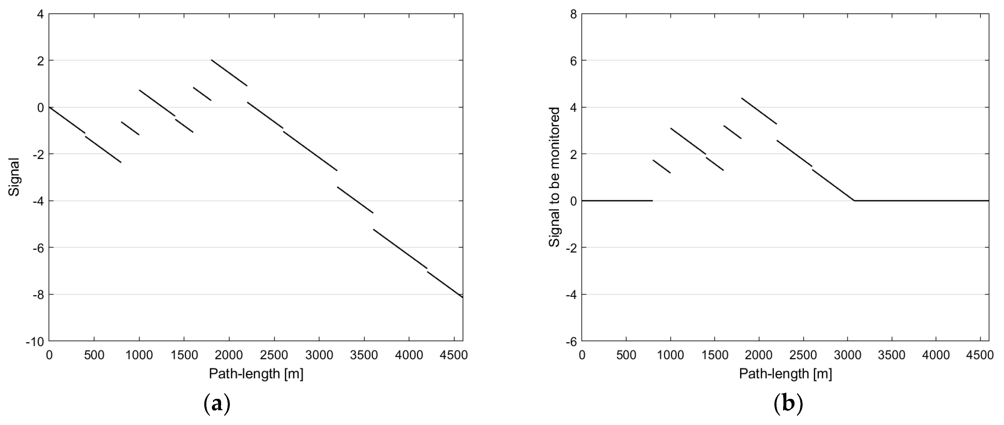
In Figure 1, functions g l D t R e s and h l D t R e s have been plotted, respectively, for the TS sequence given in Table 2. The virtual trip in this case had started from the left, as indicated by “ ” in the lower indices.
According to the diagram of h l D t R e s in Figure 1, a threshold, say, δ = 3.0 could be selected to detect the RET change. With this threshold, the change is detected at about the path-length 2.7 km, i.e., with a detection lag of 0.5 km. If smaller thresholds, e.g., δ = 1.0 or δ = 2.0 are used instead, then 3 and 1 false alarms will occur, respectively, along the 2.2 km of the Dt route. If, on the other hand, larger thresholds are used, such as δ = 4.0 or δ = 5.0 , then unnecessary extra detection lags of 0.3 and 0.6 km will occur.

3.1.2. Example No. 2: A Res → Dt Change Detector Applied to a Homologous RET Transition

To make full use of the synthetic TS sequence given in the top band of Table 2 and to provide a deeper insight into the proposed CD method, let now the ego-car start its virtual journey from the right.
As a side note, we can reverse such a virtual journey fairly easily in a table. In real life and in real traffic, however, it would be much more problematic as one might encounter very different TSs on the way back (if at all the reversed route is permitted by the TSs installed). Furthermore, the TSs that are facing us now are located on the opposite side of the road as in the first journey. However, even in case of this wieldy virtual journey, some modifications in the table, namely, with respect to the TS counts, are necessary.
These new TS counts, i.e., the counts for right-to-left virtual trips, are given in the bottom band of the table. In this reversed case, the ego-car is driven from an intended Res area to an intended Dt area, i.e., a Res → Dt transition is expected.
Again, as in the first example, we wish to form functions g T and h T that signal the RET transition that is actually expected. Accordingly, these functions are now denoted by g l R e s D t and h l R e s D t , respectively.
In order to detect such a transition, the roles of the process parameters λ k and μ k —given in the fourth and the fifth column of Table 1, respectively—need to be swapped in Equations (8) and (9), as now, it is supposed that the first road environment is a Res area, rather than a Dt area. Again, the unified counts are to be used, namely, the TS counts given in bottom band.
Functions g l R e s D t and h l R e s D t are given in Equations (14) and (15), respectively.
g l R e s D t 2.80   km 1 l + 1.74 N N S ( l ) +
+ 1.92 N P L ( l ) 0.13 N G W ( l ) 0.69 N S L ( l )
h l R e s D t = g l R e s D t inf s l g s R e s D t .
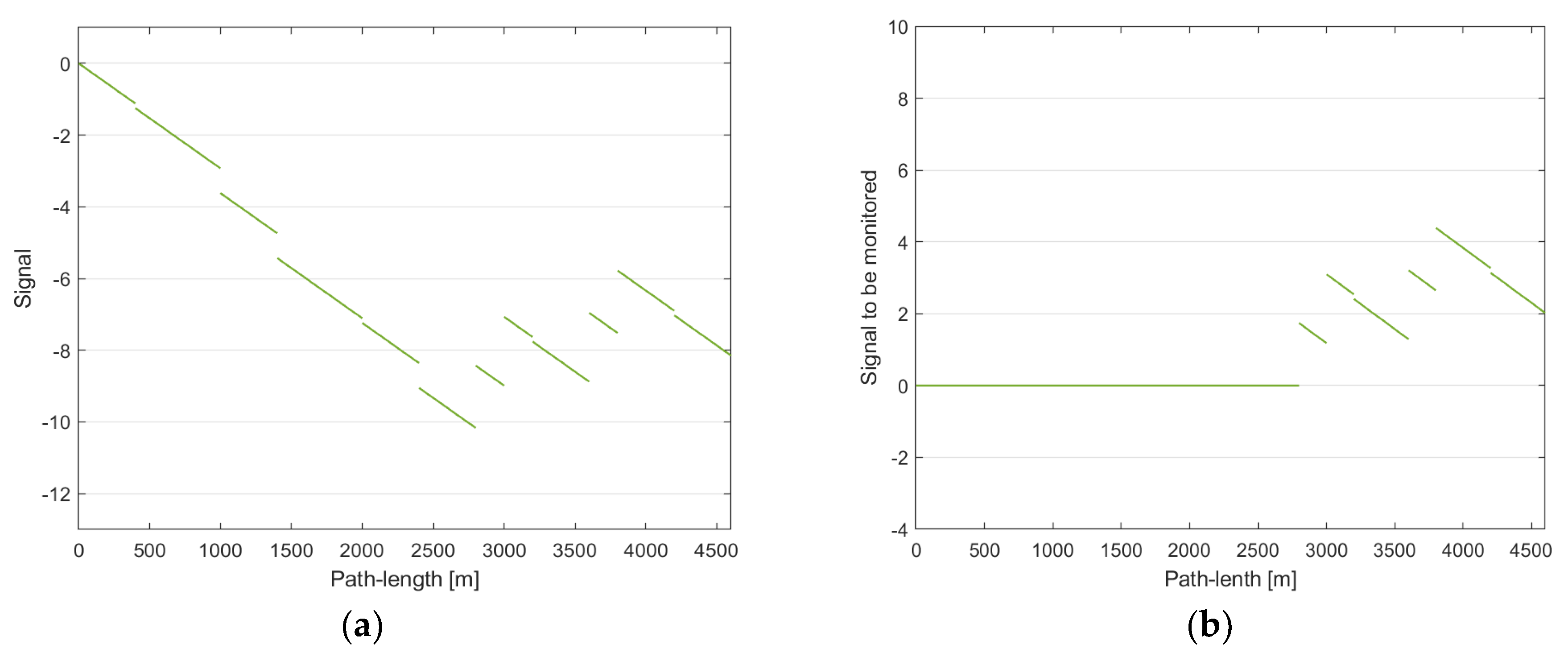
In Figure 2, the functions g l R e s D t and h l R e s D t have been plotted. The corresponding virtual journey had started from the right in the band, as indicated by the “ ” in the lower indices. The diagrams presented herein corresponding to virtual journeys from the right are presented in green.
Again, threshold δ = 3.0 would be an appropriate choice based on the diagram in Figure 2. With this threshold, the RET change is detected at about the path-length 3 km. Since the first signs of the Dt area begin to appear at the path-length 2.8 km, the detection lag is 0.2 km long.
Comparing the diagrams of g l D t R e s and g l R e s D t shown in Figure 1a and Figure 2a, respectively, one notices the symmetry between these. This symmetry can be traced back to two facts: first, from Equations (8) and (9)—as used in Example 1, and by swapping the roles of parameters λ k and μ k for equations corresponding to Example 2—furthermore, from Equations (12) and (14), it follows that
g l R e s D t 1.0 g l D t R e s .
and second, to the fact that the same route—with its TSs—was covered from opposite directions.
There will be further symmetries perceptible between the respective g l diagrams. However, similar symmetries do not show up amongst the respective h l functions.

3.2. Further Examples

In each of the two examples below, an “off-the-tune” RET change detector is considered. These change detectors are applied to the TS sequence used above, furthermore, the same marked Poisson process reference parameters are used. The examples below demonstrate that “off-the-tune” change detectors may behave fairly haphazardly. In [17], approaches are proposed to deal with such behavior of the change detectors. These approaches are essential if several differently tuned change detectors are to be used within a compound system, e.g., for the purpose of RET detection and identification, rather than CD.

3.2.1. Example No. 3: A Res → Dt Change Detector Applied to a Dt → Res Transition

Functions g l R e s D t and h l R e s D t to be used for signaling a RET transition Res → Dt have already been presented—in conjunction with the Example No. 2—in Equations (14) and (15), respectively. The only difference is that now we need to use these functions with the TS counts given in the middle band of Table 2, rather than with the TS counts given in the bottom band, as the car is now driven from the left to the right (i.e., a Dt → Res transition is expected).
In Figure 3, the diagrams of g l R e s D t and h l R e s D t are shown for an intended RET transition Dt → Res, respectively. The detector takes the first 0.8 km starting from the left for a Res area and then detects a change Res → Dt at that point (e.g., with a threshold δ = 1.0 ). If threshold δ = 3.0 is used instead, then the RET transition will be detected at 1.0 km. The corresponding detection lags for these two thresholds are 0.8 and 1.0 km, respectively. If we use larger thresholds, say, δ = 4.0 , or δ = 5.0 , then for the former, an extra detection lag of 0.9 km will be introduced, while the latter will completely miss the Dt segment of the route.
The intended RET change of transition Dt → Res remains undetected by this detector no matter what δ > 0 is used.

3.2.2. Example No. 4: A Dt → Res Change Detector Applied to a Res → Dt Transition

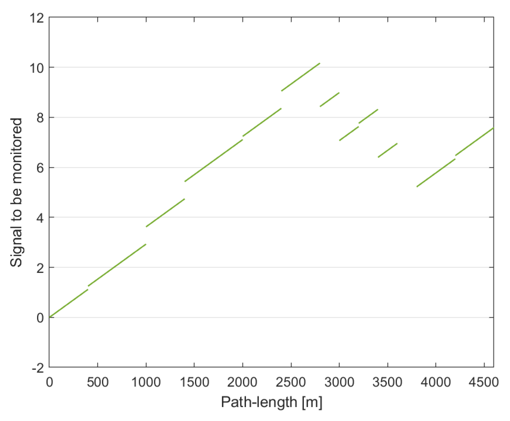
In Figure 4, the diagram of function g l D t R e s is shown for the intended RET transition Res → Dt. This transition is present when driving from the right along the considered TS sequence. Note that for the given TS sequence and for the given process parameters, functions g l D t R e s and h l D t R e s happen to be identical. Using threshold δ = 3.0 , the detector signals a change Dt → Res at about the path-length of 1 km.

4. Discussion

According to the approach derived in Section 2.2, the RET changes can be detected with CUSUM change detectors, which rely on the on-the-fly minimization effected by PHCDs.
In order to detect all kinds of the RET transitions between the three RETs considered herein, the simultaneous use of six differently tuned PHCDs is necessary. In Section 3.2, we have demonstrated what happens to the functions g l and h l when the actual RET change is not what the detector is tuned to detect. In fact, in the examples given there, we have applied change detectors that were tuned to the inverse transitions.
If one wanted to use the aforementioned PHCDs for the purpose of detecting not only the changes between different RETs, but also the actual RETs themselves, furthermore, wished to overcome the haphazard behavior of the “off-the-tune” PHCDs, there are promising possibilities; for instance, the respective functions h l can be generated and considered within a sliding window, furthermore, several overlapping sliding windows can be used at the same time. In addition, these could be multi-scale windows.
An artificial neural network (ANN) proposed for TS-based RET detection was presented in [26]. The ANN-based method made use of sliding multi-scale windows, and for these windows, TS histograms were calculated. The network proposed there could well be extended to input and make good use of the “summaries” of functions h l , rather than the TS histograms. These summaries could be of syntactic nature. A tool capable of exploring time series data for pattern and query search tasks, as well as for generating syntactic descriptions of the time series was proposed and demonstrated in [45]. The syntactic descriptions of the functions h l should preferably be computed for sliding multi-scale windows.
The TS-based RET change, the inferred actual RET within, and the complete inferred RET structure—i.e., a map layer, or sublayer—of an urban area could be utilized in various manners in automotive applications. First, the TS-based RET change, or the TS-based actual RET could initiate warnings to novice drivers, e.g., “You are now driving in a downtown area.” What actually is meant by this warning is as follows: “The area might be uncrowded now, but in half an hour, or so it could turn very busy and could be loaded with intense car traffic. Therefore, find a parking place now, if want to stay in this area.”
It also hints at reducing speed to, say, 40 km/h. In a Res area, the respective warning could, for instance, instruct the novice driver to watch out for groups of children playing on the streets.
In relation to the control of smart cars, the preferred speed could be set to some lower than 50 km/h speed in the Dt area, especially during and close to the usual peak hours. The maximum acceleration and deceleration values could be set to safer values.
In relation to the ADAS/AD computations carried out on-board smart cars, particularly to the computations related to TS detection and recognition, a specific geometrical size range for TSs can be used. In narrow streets of historical districts, often smaller TSs are installed by the road authorities, and that size should be allowed in the TS verification phase of the computing.
The detection of traffic lanes and the estimation of the distances to the TSs from the ego-car are examples for computations that implicitly make use of some spatial models of the road and its environment. In Res areas—at least in our country—multi-lane roads are infrequent, therefore simpler road structures/models should be matched against the camera images of the road scenery.
Concerning the road administration and management, the TS-based RET map layer compiled from data gathered through car-based data collection trips could be used to improve the match between seasonal, weekly, and daily traffic patterns and the inferred RETs, thereby creating a more perceivable and more self-explaining urban environment that is hopefully also safer.

5. Conclusions

The road environment appears around and sweeps past an ego-car, while it is being driven. The character of the urban road environments can be categorized into urban RETs. Abrupt changes in the character of the road environment, i.e., transitions between areas of different RETs, pose traffic safety risk, especially, for drivers lacking prolonged driving experience and also for drivers of old age.
The urban RET transitions per se manifest themselves in changes in traffic density and in the composition of the traffic. These are transient dynamic features describing an urban area, i.e., a subnetwork of an urban road network.
Nonetheless, urban RET transitions manifest themselves also in changes that concern static ROs, e.g., CRs (permanent static) and conventional TSs (transient static). So, e.g., the density and the “mixture” of TSs are expected to change between areas of different RETs. As a consequence, the RET change could also be detected via monitoring static RO occurrences along the route.
Herein, TS occurrences were considered only. These are noted in TS data logs. These logs can be interpreted as realizations of a continuous-variable IMPP, and the RET change can be detected—relying on this assumption—from them.
CD methods, e.g., the CUSUM method, are known and widely used for “simpler” inhomogeneous Poisson processes. The mentioned method was adopted and modified for detecting change between RETs based on a TS log. The behavior of the change detector was tested on a synthetic TS sequence. Nonetheless, the sequence was used in four different ways in Examples Nos. 1–4, and some observations and conclusions were drawn from these.
The presented simulation results indicate that a TS-based RET CD is feasible, and can be adopted for driver assistance, though it is not suitable for initiating an immediate intervention in critical situations.
The continuous-time approach presented herein serves as a clarification of the discrete-time model and method proposed in [25], and it was not meant and it was not expected to improve for the processing and detection characteristics achieved therein. This is due to the underlying similarity between the two stochastic models, i.e., between the marked binomial and the marked Poisson models. For this reason, the precision and the delay of the RET change detection are expected to be in the same range, respectively, for both approaches for any realistic parameter-choices in the given context.
Further research and development have been suggested in Section 4 and have been motivated with regard to the integration of the RET change detector into an ANN-based detector solution proposed earlier.

Author Contributions

Conceptualization, Z.F. and L.G.; data curation, Z.F.; formal analysis, L.G.; funding acquisition, P.G.; investigation, Z.F.; methodology, Z.F. and L.G.; project administration, P.G.; resources, P.G.; software, Z.F.; supervision, P.G.; validation, Z.F., L.G. and P.G.; visualization, Z.F.; writing—original draft, Z.F. and L.G.; writing—review and editing, P.G. All authors have read and agreed to the published version of the manuscript.

Funding

The research was supported by the Ministry of Innovation and Technology NRDI Office within the framework of the Autonomous Systems National Laboratory Program.

Institutional Review Board Statement

Not applicable.

Informed Consent Statement

Not applicable.

Data Availability Statement

Data used in the article are presented herein.

Conflicts of Interest

The authors declare no conflict of interest.

References

  1. Theeuwes, J. Self-explaining roads: Subjective categorization of road environments. In Vision in Vehicles VI; Gale, A., Brown, I.D., Taylor, S.P., Haslegrave, C.M., Eds.; Elsevier: Amsterdam, The Netherlands, 1998; pp. 279–287. [Google Scholar]
  2. Charlton, S.G.; Mackie, H.W.; Baas, P.H.; Hay, K.; Menezes, M.; Dixon, C. Using endemic road features to create self-explaining roads and reduce vehicle speeds. Accid. Anal. Prev. 2010, 42, 1989–1998. [Google Scholar] [CrossRef]
  3. Qin, Y.; Chen, Y.; Lin, K. Quantifying the effects of visual road information on drivers’ speed choices to promote self-explaining plaining roads. Int. J. Environ. Res. Public Health 2020, 17, 2437. [Google Scholar] [CrossRef] [PubMed] [Green Version]
  4. Saha, D.; Dumbaugh, E.; Merlin, L.A. A conceptual framework to understand the role of built environment on traffic safety. J. Saf. Res. 2020, 75, 41–50. [Google Scholar] [CrossRef] [PubMed]
  5. Ding, H.; Zhao, X.; Rong, J.; Ma, J. Experimental research on the effectiveness of speed reduction markings based on driving simulation: A case study. Accid. Anal. Prev. 2013, 60, 211–218. [Google Scholar] [CrossRef]
  6. Banach, M.; Długosz, R. Techniques to facilitate the use of V2I communication system as support for traffic sign recognition algorithms. In Proceedings of the 24th International Conference on Methods and Models in Automation and Robotics, Miedzyzdroje, Poland, 26–29 August 2019; pp. 308–313. [Google Scholar]
  7. Ahangar, M.N.; Ahmed, Q.Z.; Khan, F.A.; Hafeez, M. A survey of autonomous vehicles: Enabling communication technologies and challenges. Sensors 2021, 21, 706. [Google Scholar] [CrossRef] [PubMed]
  8. Popescu, O.; Sha-Mohammad, S.; Abdel-Wahab, H.; Popescu, D.C.; El-Tawab, S. Automatic incident detection in intelligent transportation systems using aggregation of traffic parameters collected through V2I communications. IEEE Intell. Transp. Syst. Mag. 2017, 9, 64–75. [Google Scholar] [CrossRef]
  9. Sattar, F.; Karray, F.; Kamel, M.; Nassar, L.; Golestan, K. Recent advances on context-awareness and data/information fusion in ITS. Int. J. Intell. Transp. Syst. Res. 2016, 14, 1–19. [Google Scholar] [CrossRef]
  10. Global Navigation Satellite System (GNSS) Devices per Capita Worldwide 2019–2029. Available online: https://www.statista.com/statistics/1174568/gnss-devices-per-capita-worldwide/#statisticContainer (accessed on 21 March 2021).
  11. Reid, T.G.; Chan, B.; Goel, A.; Gunning, K.; Manning, B.; Martin, J.; Tarantino, P. Satellite navigation for the age of autonomy. In Proceedings of the 2020 IEEE/ION Position, Location and Navigation Symposium, Portland, OR, USA, 20–23 April 2020; pp. 342–352. [Google Scholar]
  12. Schmidt, D.; Radke, K.; Camtepe, S.; Foo, E.; Ren, M. A survey and analysis of the GNSS spoofing threat and countermeasures. ACM Comput. Surv. 2016, 48, 64. [Google Scholar] [CrossRef]
  13. Welzel, A.; Reisdorf, P.; Wanielik, G. Improving urban vehicle localization with traffic sign recognition. In Proceedings of the 18th IEEE International Conference on Intelligent Transportation Systems, Gran Canaria, Spain, 15–18 September 2015; pp. 2728–2732. [Google Scholar]
  14. The Traffic Safety Problem in Urban Areas. Available online: http://citeseerx.ist.psu.edu/viewdoc/download?doi=10.1.1.572.9092&rep=rep1&type=pdf (accessed on 9 December 2020).
  15. Wechsler, K.; Drescher, U.; Janouch, C.; Haeger, M.; Voelcker-Rehage, C.; Bock, O. Multitasking during simulated car driving: A comparison of young and older persons. Front. Psychol. 2018, 9, 910–921. [Google Scholar] [CrossRef]
  16. Faure, V.; Lobjois, R.; Benguigui, N. The effects of driving environment complexity and dual tasking on drivers’ mental workload and eye blink behavior. Transp. Res. Part F Traffic Psychol. Behav. 2016, 40, 78–90. [Google Scholar] [CrossRef]
  17. Payyanadan, R.P.; Lee, J.D.; Grepo, L.C. Challenges for older drivers in urban, suburban, and rural settings. Geriatrics 2018, 3, 14. [Google Scholar] [CrossRef] [Green Version]
  18. Tawari, A.; Sivaraman, S.; Trivedi, M.M.; Shannon, T.; Tippelhofer, M. Looking-in and looking-out vision for urban intelligent assistance: Estimation of driver attentive state and dynamic surround for safe merging and braking. In Proceedings of the IEEE Intelligent Vehicles Symposium, Dearborn, MI, USA, 8–11 June 2014; pp. 115–120. [Google Scholar]
  19. Stapel, J.; El Hassnaoui, M.; Happee, R. Measuring driver perception: Combining eye-tracking and automated road scene perception. Hum. Factors. 2020. [Google Scholar] [CrossRef]
  20. Tang, R.; Jiang, Z. Driver’s perception model in driving assist. In Proceedings of the IEEE 20th International Conference on Software Quality, Reliability and Security Companion, Macau, China, 11–14 December 2020; pp. 237–240. [Google Scholar]
  21. Rudin-Brown, C.M.; Edquist, J.; Lenne, M.G. Effects of driving experience and sensation-seeking on drivers’ adaptation to road environment complexity. Saf. Sci. 2014, 62, 121–129. [Google Scholar] [CrossRef]
  22. Lin, H.; Gao, J.; Zhou, Y.; Lu, G.; Ye, M.; Zhang, C.; Liu, L.; Yang, R. Semantic decomposition and reconstruction of residential scenes from LiDAR data. ACM Trans. Graph. 2013, 32, 1–10. [Google Scholar] [CrossRef]
  23. Wang, Y.; Cheng, L.; Chen, Y.; Wu, Y.; Li, M. Building point detection from vehicle-borne LiDAR data based on voxel group and horizontal hollow analysis. Remote Sens. 2016, 8, 419. [Google Scholar] [CrossRef] [Green Version]
  24. Jeong, J.; Cho, Y.; Shin, Y.-S.; Roh, H.; Kim, A. Complex urban dataset with multi-level sensors from highly diverse urban environments. Int. J. Rob. Res. 2019, 38, 642–657. [Google Scholar] [CrossRef] [Green Version]
  25. Fazekas, Z.; Balázs, G.; Gerencsér, L.; Gáspár, P. Inferring the actual urban road environment from traffic sign data using a minimum description length approach. Transp. Res. Proc. 2017, 27, 516–523. [Google Scholar] [CrossRef]
  26. Fazekas, Z.; Balázs, G.; Gáspár, P. ANN-based classification of urban road environments from traffic sign and crossroad data. Acta Polytech. Hung. 2018, 15, 83–100. [Google Scholar]
  27. SAFESPOT Final Report 2010. Available online: http://www.safespot-eu.org/documents/D8.1.1_Final_Report_-_Public_v1.0.pdf (accessed on 22 March 2021).
  28. Map Features. Available online: https://wiki.openstreetmap.org/wiki/Map_features (accessed on 8 April 2021).
  29. Liu, X.; Gong, L.; Gong, Y.; Liu, Y. Revealing travel patterns and city structure with taxi trip data. J. Transp. Geogr. 2015, 43, 78–90. [Google Scholar] [CrossRef] [Green Version]
  30. Kastner, R.; Michalke, T.; Adamy, J.; Fritsch, J.; Goerick, C. Task-based environment interpretation and system architecture for next generation ADAS. IEEE Trans. Intell. Transp. Syst. 2011, 3, 20–33. [Google Scholar] [CrossRef]
  31. Sindhu, O.S.S.V.; Victer, P.P. Computer vision model for traffic sign recognition and detection: A survey. In Proceedings of the International Conference on Communications and Cyber Physical Engineering, Hyderabad, India, 24–25 January 2018; pp. 679–690. [Google Scholar]
  32. Veronese, L.P.; Badue, C.; Cheein, F.A.; Guivant, J.; De Souza, A.F. A single sensor system for mapping in GNSS-denied environments. Cogn. Syst. Res. 2019, 56, 246–261. [Google Scholar] [CrossRef]
  33. Lin, C.C.; Wang, M.S. Road sign recognition with fuzzy adaptive pre-processing models. Sensors 2012, 12, 6415–6433. [Google Scholar] [CrossRef]
  34. Kim, T.; Park, T.-H. Extended Kalman Filter (EKF) design for vehicle position tracking using reliability function of Radar and Lidar. Sensors 2020, 20, 4126. [Google Scholar] [CrossRef]
  35. Akhlaq, M.; Sheltami, T.R.; Helgeson, B.; Shakshuki, E.M. Designing an integrated driver assistance system using image sensors. J. Intell. Manuf. 2012, 23, 2109–2132. [Google Scholar] [CrossRef]
  36. Belbachir, A. An embedded testbed architecture to evaluate autonomous car driving. Intell. Serv. Robot. 2017, 10, 109–119. [Google Scholar] [CrossRef]
  37. Manual for Streets, Department for Transport and Ministry of Housing, Communities & Local Government, UK, 29 March 2007. Available online: https://assets.publishing.service.gov.uk/government/uploads/system/uploads/attachment_data/file/341513/pdfmanforstreets.pdf (accessed on 22 March 2021).
  38. Roads 2018. Available online: https://ec.europa.eu/transport/road_safety/sites/roadsafety/files/pdf/ersosynthesis2018-roads.pdf (accessed on 22 March 2021).
  39. Kingman, J.F.C. Poisson processes. In Encyclopedia of Biostatistics; Armitage, P., Colton, T., Eds.; Wiley and Sons: Hoboken, NJ, USA, 2005. [Google Scholar]
  40. Poor, H.V.; Hadjiliadis, O. Quickest Detection; Cambridge University Press: Cambridge, UK, 2008. [Google Scholar]
  41. Tartakovsky, A.; Nikiforov, I.; Basseville, M. Sequential Analysis: Hypothesis Testing and Change Detection; Chapman and Hall/CRC: New York, NY, USA, 2014. [Google Scholar]
  42. Page, E.S. Continuous inspection schemes. Biometrika 1954, 41, 100–115. [Google Scholar] [CrossRef]
  43. Hinkley, D.V. Inference about the change-point in a sequence of random variables. Biometrika 1970, 57, 1–17. [Google Scholar] [CrossRef]
  44. Gerencsér, L.; Prosdocimi, C. Input-output properties of the Page-Hinkley detector. Syst. Control Lett. 2011, 60, 486–491. [Google Scholar] [CrossRef]
  45. Rodrigues, J.; Folgado, D.; Belo, D.; Gamboa, H. SSTS: A syntactic tool for pattern search on time series. Inf. Process. Manag. 2019, 56, 61–76. [Google Scholar] [CrossRef]
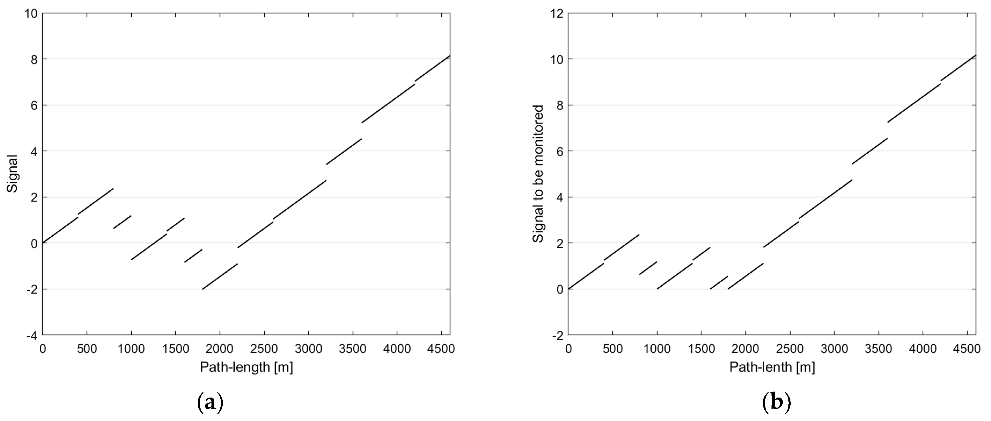
Figure 1. A downtown (Dt) → residential (Res) change detector applied to a homologous road environment type (RET) transition showing up in the traffic sign (TS) sequence given in the top band of Table 2: (a) Function g l D t R e s for the considered TS sequence and (b) Function h l D t R e s .
Applsci 11 03666 g001
Figure 2. A Res → Dt change detector applied to a homologous RET transition appearing in the TS sequence given in the top band of Table 2: (a) Function g l R e s D t for the considered TS sequence and (b) Function h l R e s D t .
Applsci 11 03666 g002
Figure 3. A Res → Dt change detector applied to a Dt → Res transition showing up in the TS sequence given in the top band of Table 2: (a) Function g l R e s D t for the considered TS sequence and (b) Function h l R e s D t .
Applsci 11 03666 g003
Figure 4. Function g l D t R e s for the considered TS sequence. For the given sequence and for the given process parameters functions g l D t R e s and h l D t R e s happen to be identical.
Applsci 11 03666 g004
Table 1. The empirical traffic sign (TS) rates along a random route for the homogeneous marked Poisson processes describing (downtown) Dt and residential (Res) urban road environments.
TS TypeAbbeviationIndex Expected Number
of Occurrences
per km in Dt
Expected Number of Occurrences per km in Res AreasNatural Logarithm of the Rate-RatioCharacteristic to
Applsci 11 03666 i001NS12.000.351.74Dt
Applsci 11 03666 i002PL21.700.251.92Dt
Applsci 11 03666 i003GW30.700.80−0.13Res
Applsci 11 03666 i004SL40.200.40−0.69Res
Any 4.601.80 Dt
Table 2. A synthetic sequence of TSs used in the examples (top band), and the unified counts for the No stopping (NS), Parking lot (PL), the Give way (GW), and Max speed 30 km/h (SL) TSs in case of trips starting from the left and from the right, respectively (middle and bottom bands).
—— Applsci 11 03666 i003—— Applsci 11 03666 i001 Applsci 11 03666 i002—— Applsci 11 03666 i003 Applsci 11 03666 i002 Applsci 11 03666 i001—— Applsci 11 03666 i004———— Applsci 11 03666 i003——— Applsci 11 03666 i004—— Applsci 11 03666 i004——— Applsci 11 03666 i003——
1 2
1 2
1 2 3 4
1 2 3
2 1
2 1
4 3 2 1
3 2 1
Publisher’s Note: MDPI stays neutral with regard to jurisdictional claims in published maps and institutional affiliations.