The Investigation on the Flow Distortion Effect of Header to Guarantee the Measurement Accuracy of the Ultrasonic Gas Flowmeter

Featured Application

This study investigated the flow distortion effect of the header on the measurement accuracy of the ultrasonic gas flowmeter by experiments and CFD, and the physical mechanism of characteristic parameters on measurement accuracy was explored.

Abstract

The quantification of the flow distortion effect on the measurement accuracy of the ultrasonic gas flowmeter downstream of the header is important but an area that has been of less concern in the research. By experiments and computational fluid dynamics (CFD), the influence of flow field distortion was studied. Experimental results under three different installation conditions showed that when there was flow field distortion downstream of the header, the measurement results of the gas ultrasonic flowmeter were 1% higher than those when there was no distortion, while a flow conditioner could effectively eliminate flow field distortion. Based on the experimental tests, the flow field distribution was analyzed with CFD, which showed that the flow field distortion effect generated by the header had a significant influence on the parameter of nonconforming Profile factor, while the parameters of Symmetry and Cross-flow could be obviously eliminated by the double-cross-section designing.

1. Introduction

Accurate measurement of the volume of fluid passed is a critical requirement for custody transfer. The measurement error can result in serious financial losses for either the buyer or seller [1]. Ultrasonic gas flow detection technology is a research hotspot in the field of flow detection in recent years [2]. Due to the unique advantages over other measuring instruments in measurement accuracy, reliability, pressure loss, maintenance cost, and manufacturing cost [3,4], the transit-time multipath ultrasonic flowmeter (TM-USM), taking the places of the traditional mechanical flow meters, has become the best choice [5,6], especially in the field of custody-transfer applications of natural gas.

The working principle of TM-USM is shown in Equations (1)–(3) and Figure 1 [7,8], where v is the inlet flow velocity, L is the propagation path length, D is the pipe diameter, φ is the path angle, c is the sound velocity, and i represents a different path. The flow velocity of each path can be calculated by the difference between the downstream propagation time t_d and upstream propagation time t_u:

$$t_{di}=\frac{L_i}{c+v_i\cos \phi }$$

(1)

$$t_{ui}=\frac{L_i}{c-v_i\cos \phi }$$

(2)

$$v_i=\frac{L_i}{2\cos \phi }\left(\frac{1}{t_{di}}-\frac{1}{t_{ui}}\right)$$

(3)

The research on USM was mainly focused on two aspects. The first aspect was the continuous improvement of the structure of USM itself, such as using multi-path ultrasonic flowmeters [9,10], optimizing the layout of paths, weights of the acoustic paths [11,12], the installation angle of the transducers [13,14], multiple reflections of ultrasonic signals in the pipe [8], and so on. There are many manufacturers that all had different types of USMs with stable performance on the market [3,15,16]. However, the accurate measurement of USMs largely depended on the full development of flow profile in the pipeline [17,18,19]. The flow profile could be affected by distortions caused by the practical limitations of industry sites, space constrains, various upstream pipe configurations [20,21], or recess and protrusion of the transducers [13,22]. It would produce additional measurement errors up to several times relative to the designed value. Therefore, another aspect of the research on USMs was focused on the influence of the flow field distribution on the measurement accuracy of USMs in use.

In recent years, a lot of research had been carried out on improving the measurement accuracy of USMs resulted from flow field distortion by the means of experiment [23,24,25], theoretical derivation [8,20,26], and CFD simulation [16,27,28].

John Lansing et al. discussed an eight-path ultrasonic meter to identify what uncertainties remain from installations. They presented data on installations with and without a flow conditioner. In addition to presenting information on the effect this upstream piping disturbance had on the meter’s accuracy, data were published on what the impact might be with some blockage in front of the flow conditioner [10,29]. Hui Zhang et al. emphasized the effects of velocity profiles across the pipe on the propagation time of ultrasonic wave; theoretical flowrate correction factors considering the real velocity profile were proposed for laminar and turbulent flow to obtain higher accuracy. The experiment data of an ultrasonic flowmeter and weighting method are compared to verify the proposed theoretical correction factors [30]. Huichao Zhao et al. explored the influence of complex flow profiles on the performance of a multipath ultrasonic flow meter by using the CFD simulation. It was shown that the characteristic parameters of swirling number and asymmetry ratio could describe the distorted pipe flow with secondary flow effectively and may be helpful for the monitoring of multipath ultrasonic flow meter cause by complex pipe configurations [31].

In the aforementioned documents, the research objects were mostly typical pipe configurations such as single elbows, double elbows, and reduced diameter pipes [32,33], etc., which were specified in international recommendation OIML R137.

In practice, as an indispensable part of the natural gas transport station or standard flow device, the pipe header was usually used to buffer and balance the inlet medium pressure and flow of all parties, and transport it downstream after the parameters were stabilized. However, if the downstream straight pipe length was not long enough, the header would also become a kind of disturbing facility. There were few research contents on headers, while most of them were based on CFD simulation.

To quantifiably investigate the flow distortion effect of the header, the accurate measurement results of USM were carried out on flow standard devices under different flow distribution conditions downstream from the header. Based on the tests, the CFD was used to investigate the flow distortion effect of header on USMs.

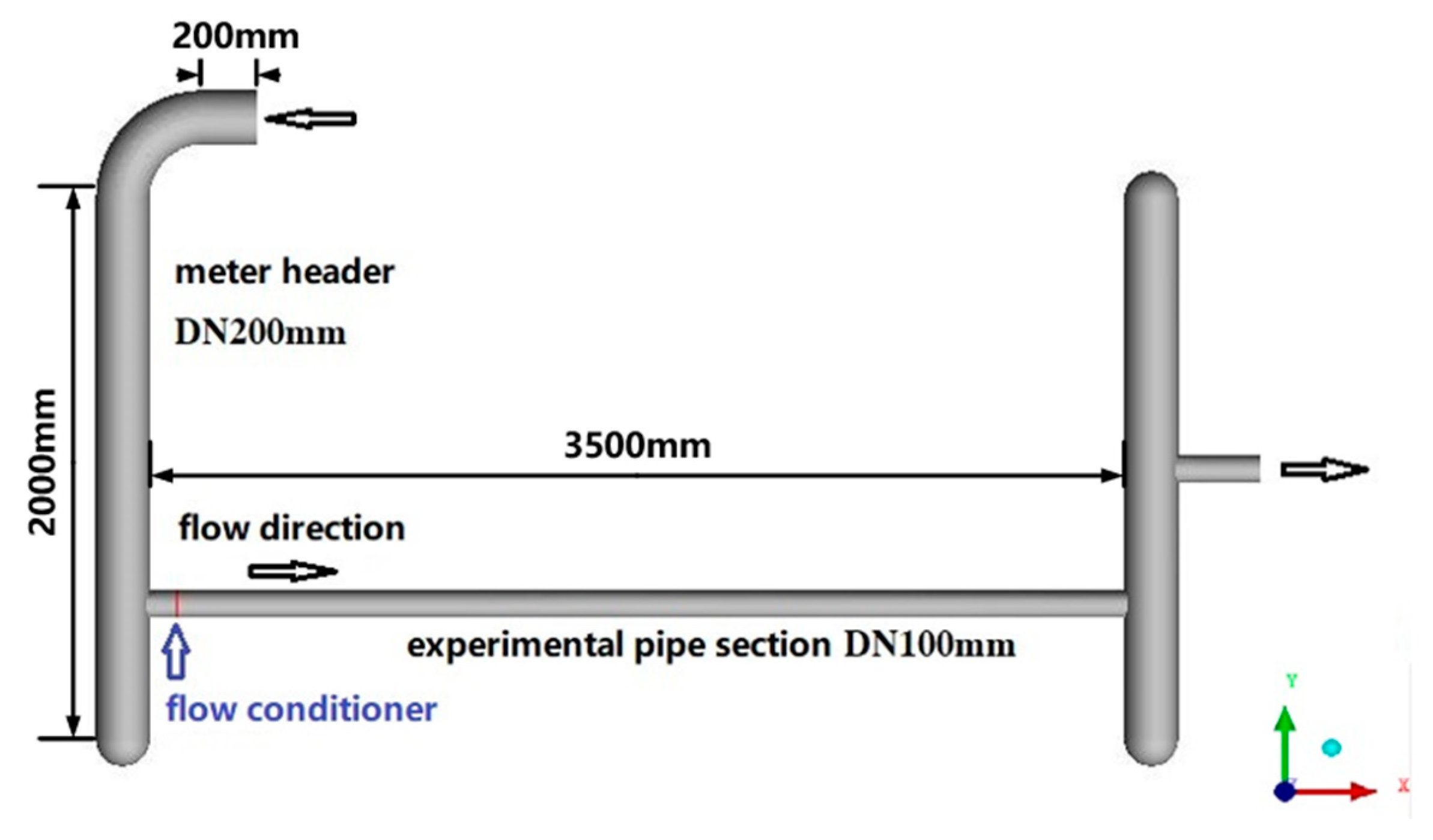
2. The Experiment Facilities

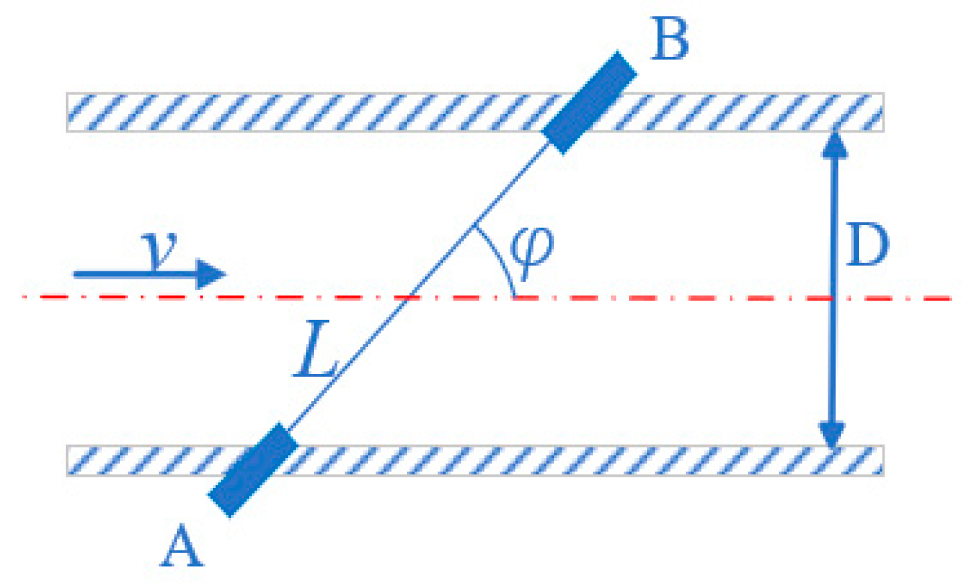
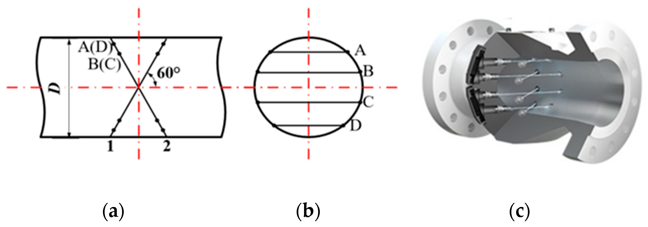
2.1. The Meter under Test

The flowmeter used in this experiment was a double-cross-section/eight-path USM, while the diameter was 100 mm, as shown in Figure 2. This USM had 16 transducers comprising eight paths arranged in four chordal planes, each at ±60° to the axis of the pipe [34]. From top to bottom, the four paths were named as A, B, C, and D respectively.

The path position was arranged according to the Gauss–Jacobi integration scheme, as shown in

Table 1. Path position and path weight.

Number of Paths	Gauss–Jacobi Positions xi = di/R	Gauss–Jacobi Weights (4 Path) wi	Velocity Weights (4/8 Path) Wi
A(1-A/2-A)	0.8090	0.3693	0.1382/0.0691
B(1-B/2-B)	0.3090	0.5976	0.3618/0.1809
C(1-C/2-C)	−0.3090	0.5976	0.3618/0.1809
D(1-D/2-D)	−0.8090	0.3693	0.1382/0.0691

Here, d_i was the path height, which referred to the vertical distance of the path line from the pipe axis, and x_i was the corresponding path height ratio.

[35]. The average surface velocity was the weighted sum of the velocities along the individual paths. For a single measurement section, there were:

$$Q=KR{\displaystyle \sum _{i=1}^n{w}_i{v}_i{L}_{wi}\sin \phi }=K^{\prime }\cdot \pi {\frac{D}{4}}^2{\displaystyle \sum _{i=1}^n{W}_i{v}_i}$$

(4)

where Q was the volumetric flow, K and K′ were the correction factors, which were used to make up for the error caused by the conversion from linear average velocity to surface average velocity [36], R was the inner pipe radius, w_i was the Gauss–Jacobi weighting factor of path i, v_i was the average line velocity measured on path i, L_wi was the theoretical path length, namely the distance between the two probes, φ was the angle between the path line and the axis of the pipe, D was the inner diameter of the meter, W_i was the velocity weighting factor of path i, which was transformed from the Gauss–Jacobi weighting factor and widely used by manufacturers, and n was the number of paths. For a two-section measurement, the final flow rate was the average of the measured volumetric flow rates of the two sections.

2.2. The Test Facility

At the end of 2014, the high-pressure gas system was built in National Institute of Metrology of China (NIM), which consisted of 3 sections, including a pVTt primary standard device, sonic nozzle secondary standard device, and close loop working standard device. The maximum pressure in the system could be 2.5 MPa.

➢

For the sonic nozzle secondary standard device (SN device), there were 16 sonic nozzles used as the masters, as shown in Figure 3. The sonic nozzles were traceable to the pVTt primary standard device. The flowrate could be (20~400) m³/h with the best measurement capabilities 0.15% (k = 2) [37].

➢

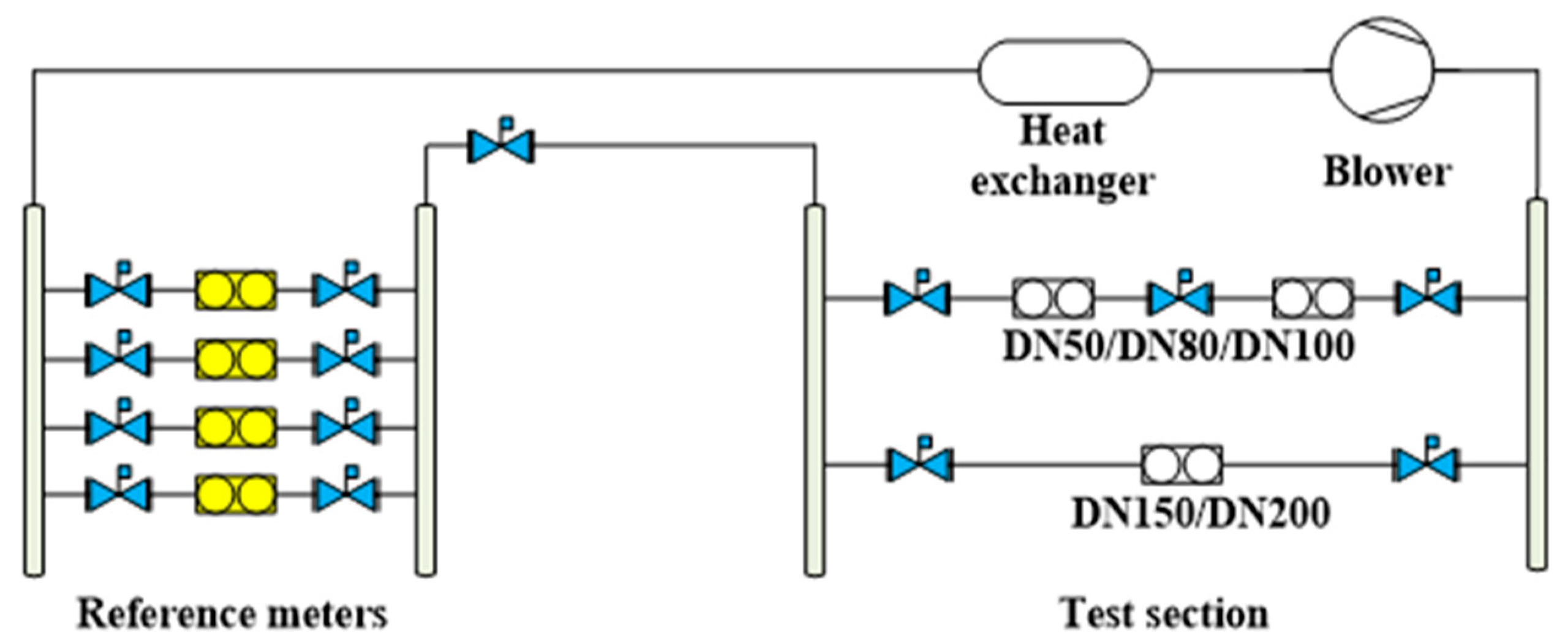
For the close loop working standard device (CL device), there were four turbine flowmeters used as the reference meters, as shown in Figure 4. The high-pressure gas was recirculated in the standard device, which was driven by the blower and the temperature was controlled by the heat exchanger. The reference meters were traceable to the sonic nozzle secondary standard device. The maximum flowrate could be 1300 m³/h with the best measurement capabilities 0.18% (k = 2) [38].

The structure of experimental section of the SN device and CL device were the same, both the upstream and downstream were headers, and there were no other disturbing facilities in the pipeline.

There were 3 installation conditions of USM designed to investigate the distortion effect resulted from header:

➢

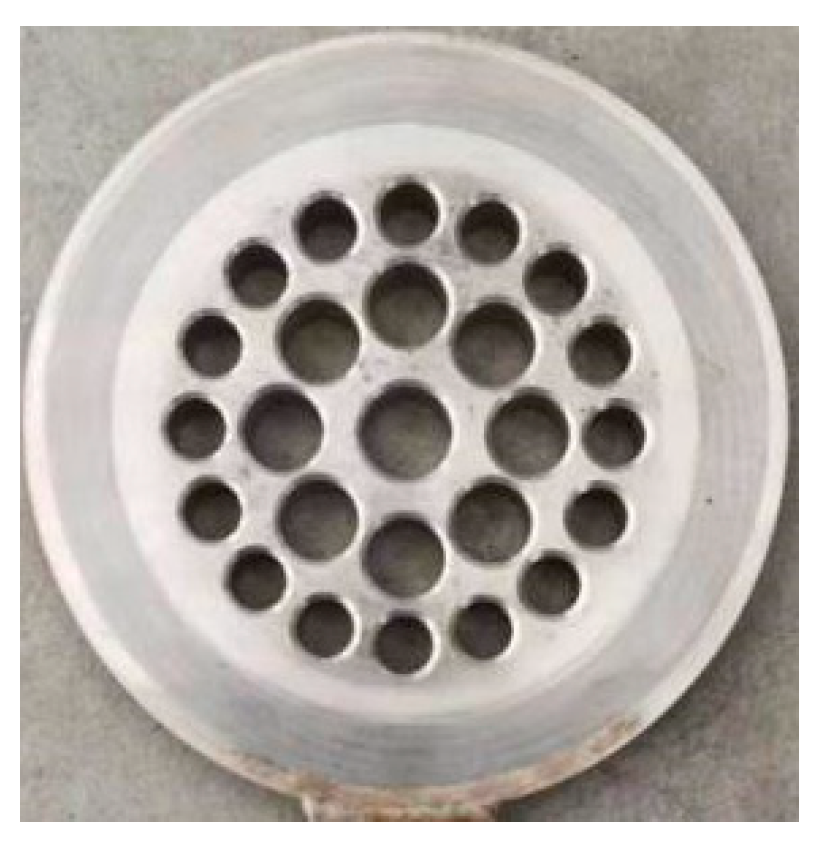
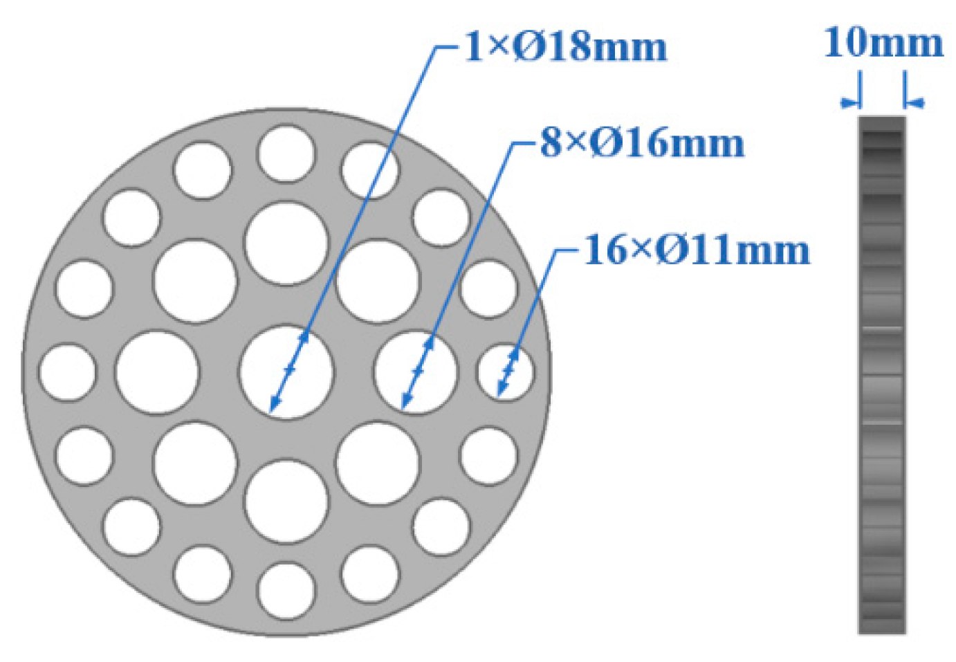
The 36D upstream pipe length with an orifice plate flow conditioner (FC) as shown in Figure 5, which was conducted in the CL device;

➢

The 19D upstream pipe length with an FC, which was conducted in the SN device;

➢

The 19D upstream pipe length, which was also conducted in the SN device but without FC.

In this paper, the experiments of USM were carried out on the CL device and SN device under different installation conditions at 0.36 MPa and 2.5 MPa in order to study the effect of headers. Five flow points were selected for each experiment, and each point was repeated 4 times.

3. The Experiment Results

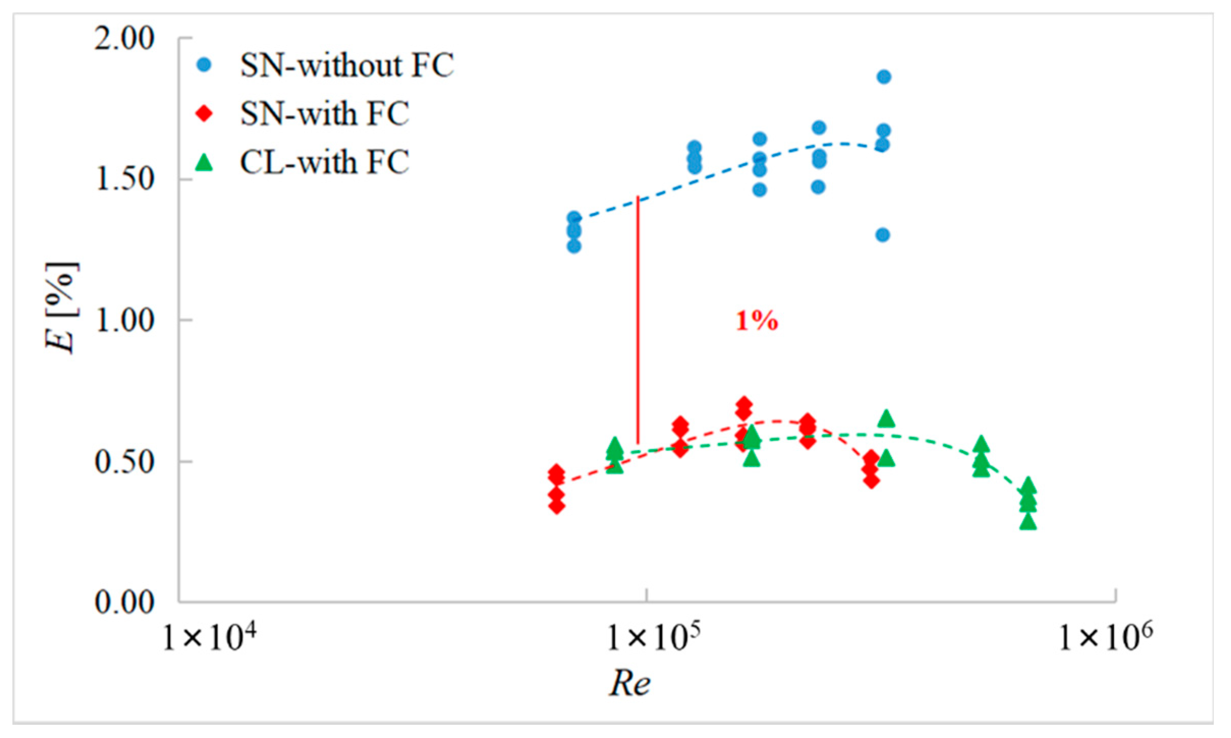
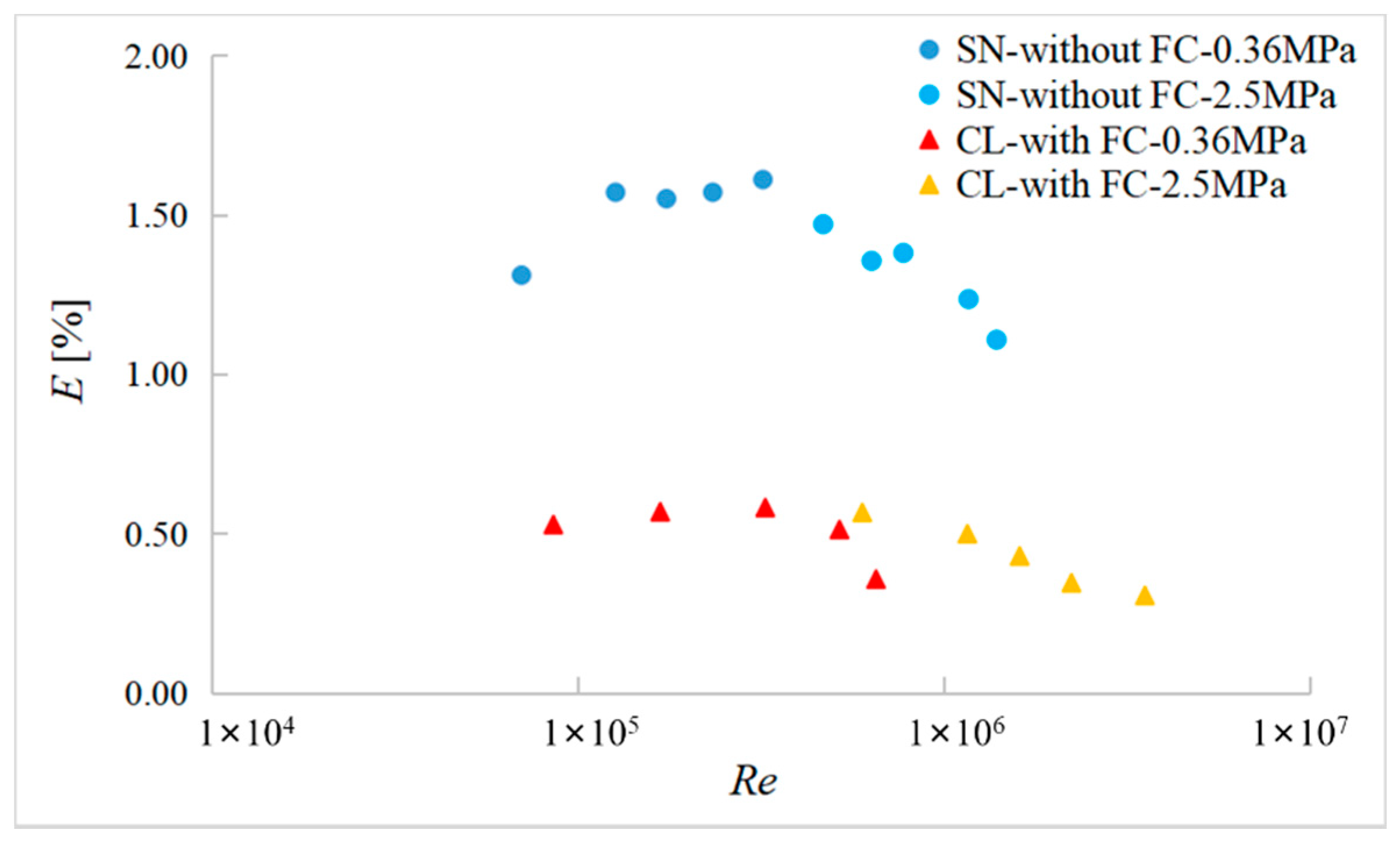
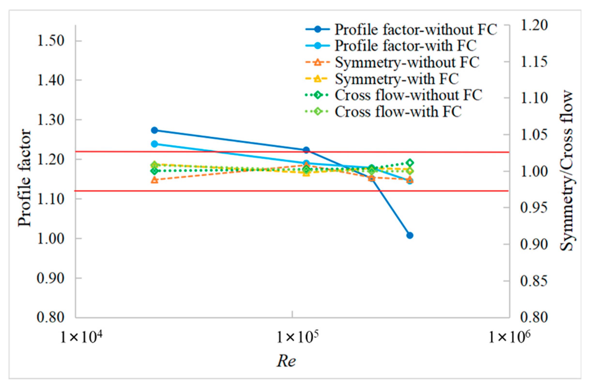
3.1. The Measurement Errors

Here, E, the measurement error of USM, was used to express the deviation between the indication flow rate Q_ind of USM and the reference flow Q_ref of the standard device [39,40].

$$E=\frac{Q_{\mathrm{ind}}-Q_{\mathrm{ref}}}{Q_{\mathrm{ref}}}\times 100\%$$

(5)

Figure 6 showed that the measurement results of USM under conditions 1 and 2 were about 0.5%. It showed the consistency between the SN device and the CL device, while it had already been verified with a turbine meter [38]. However, for the SN device, the measurement errors without FC were about 1.5%, which were obviously higher than those with FC at the same Reynolds number. The difference could be 1% at 0.36 MPa, and the measurement results without FC were relatively scattered.

It could be seen from Figure 7 that the differences between two devices under different installation conditions were decreased with the increasing of Reynolds number, but they were still much higher than the uncertainty of the best measurement capabilities 0.15% (k = 2).

The header was the only disturbing component in the experiments. Without the FC, the serious flow distortion would occur downstream from the header, resulting in additional measurement errors. With the FC, the measurement accuracy could be greatly improved.

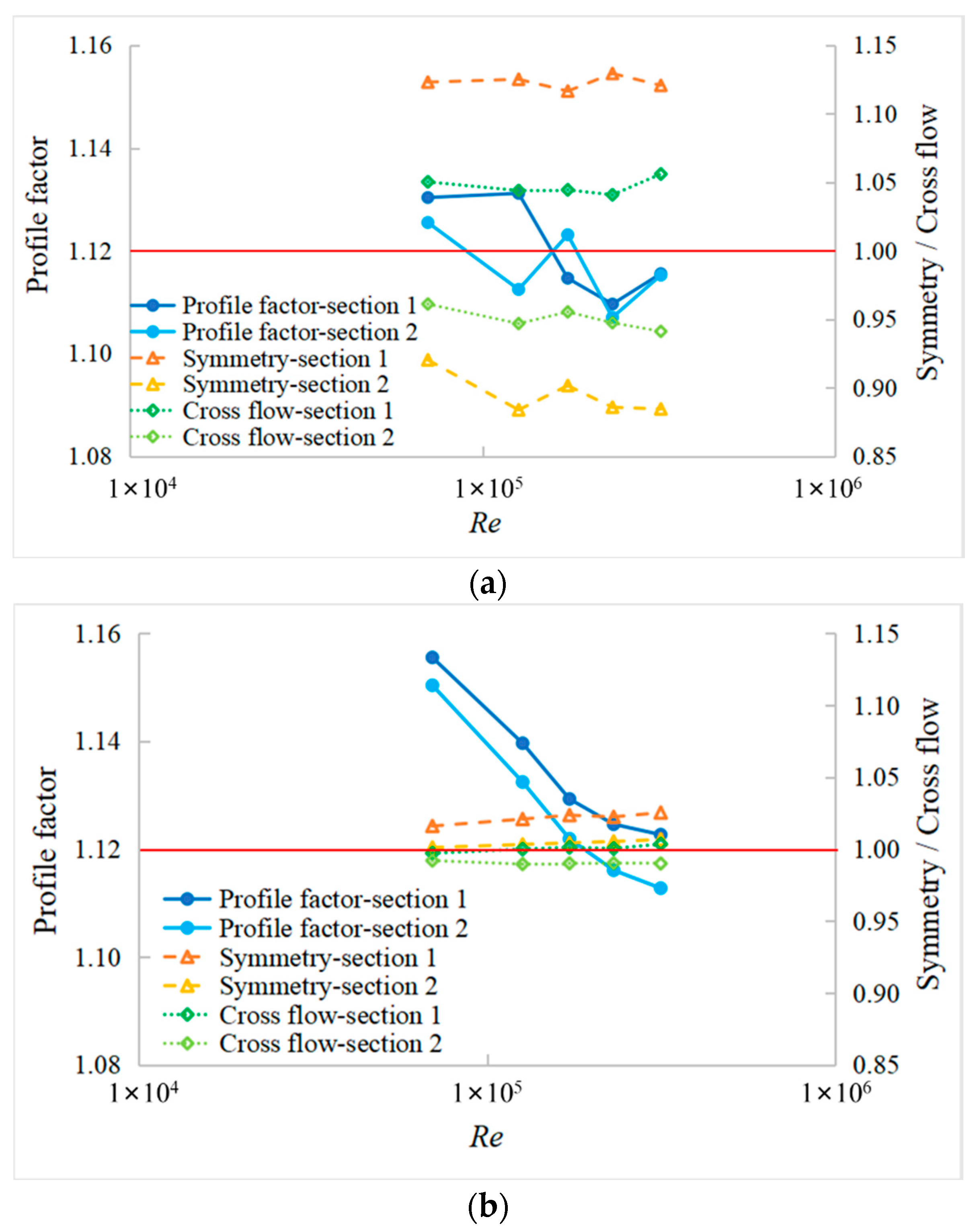
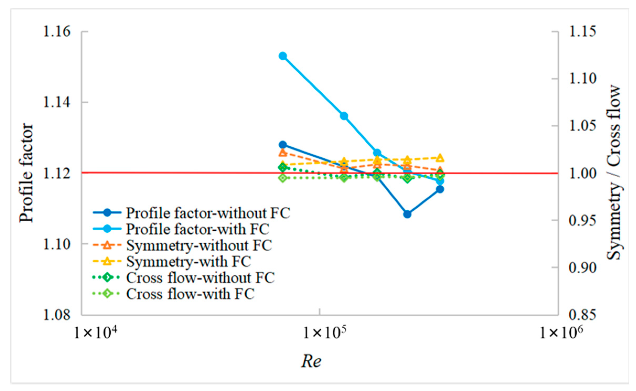
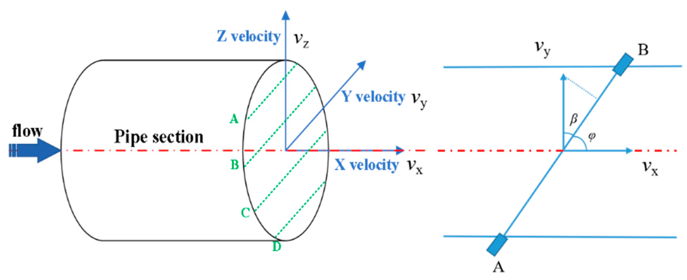
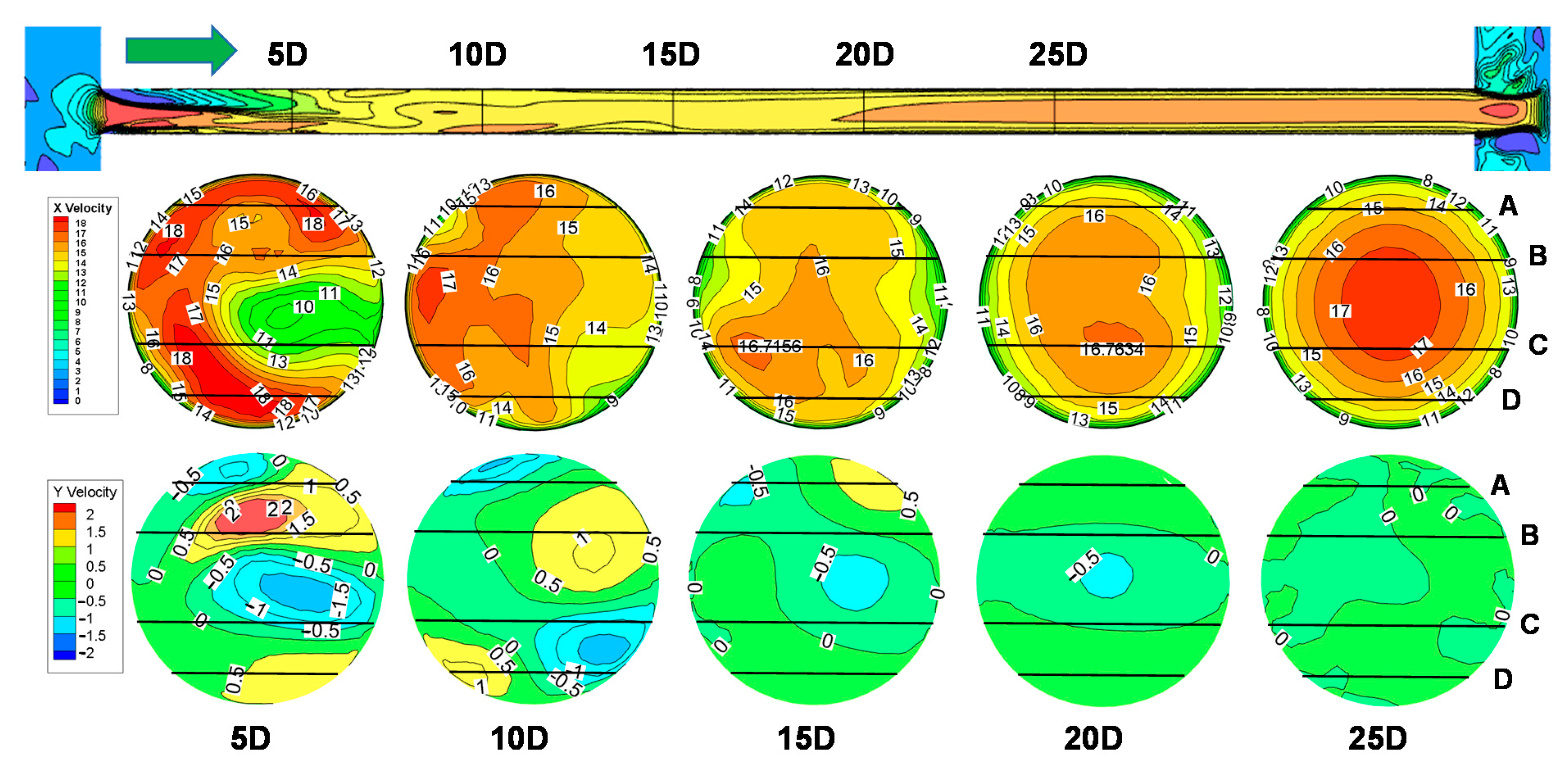
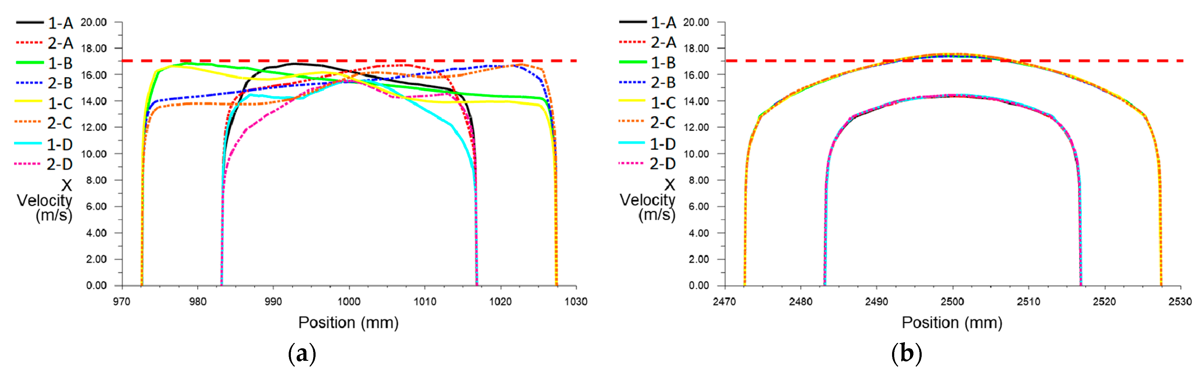
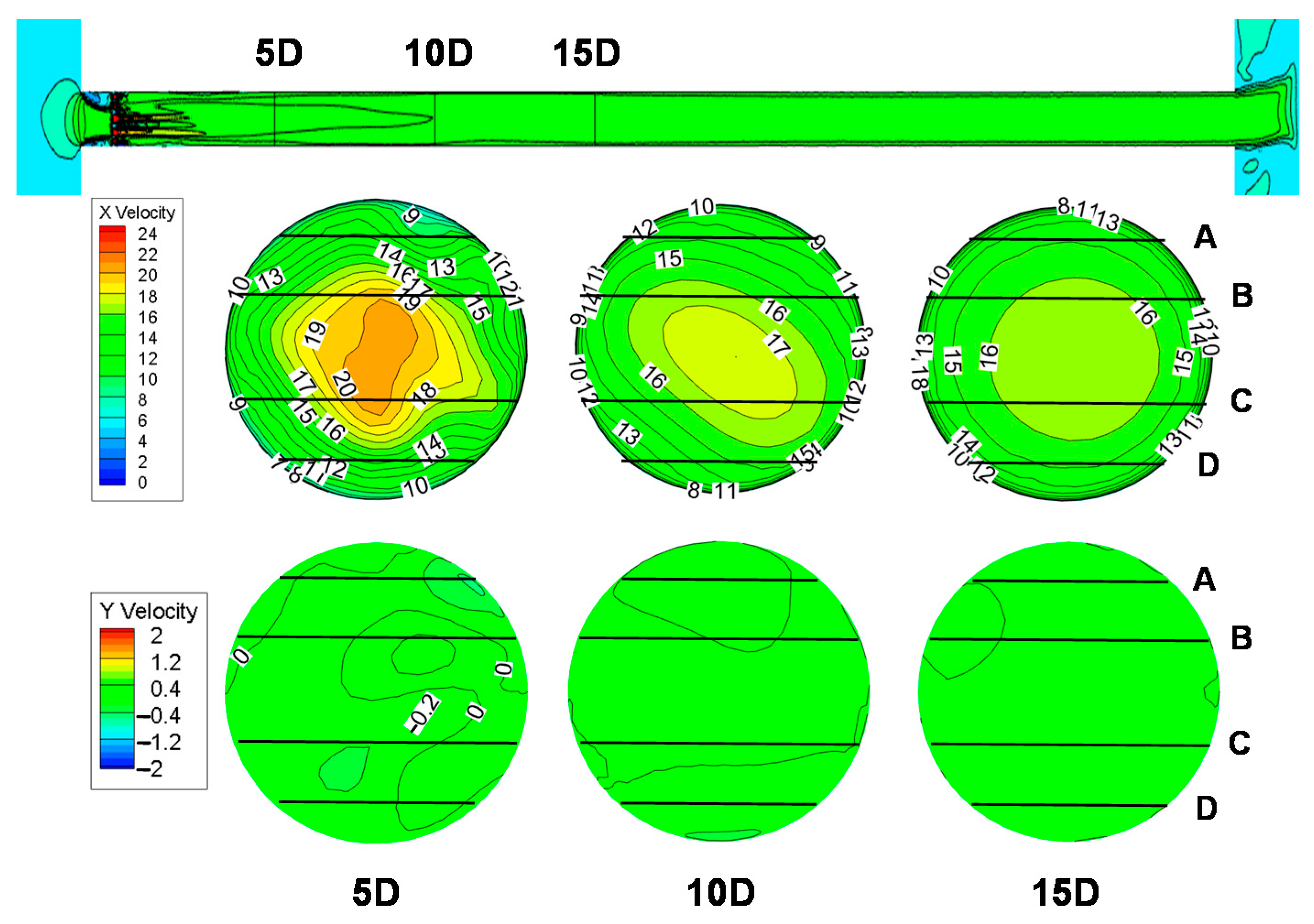
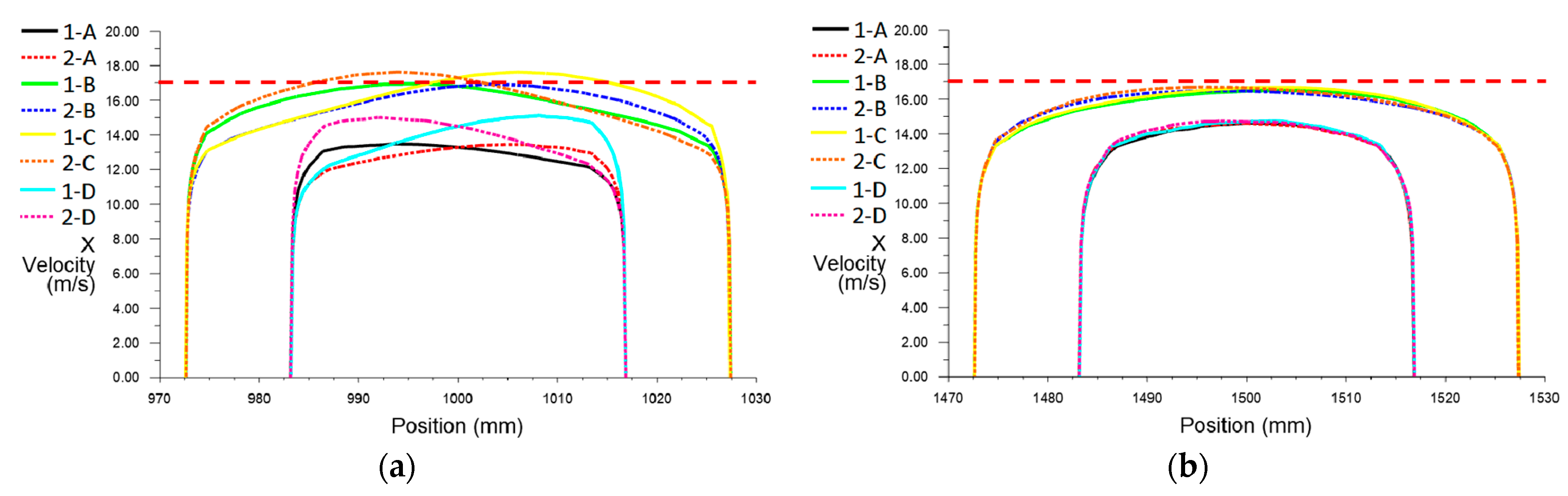
3.2. The Flow Distribution in Different Sections

In addition to the volume flow rate and average velocity, the velocity along each path also provided information about the flow distribution. Here, the definition and quantification of flow characteristic parameters expressing the types of perturbations developed were as follows, which were also used by most manufacturers to qualify the flow state [41,42]:

➢

Profile factor: described the distribution of axial flow in the pipe, and it was therefore a quantification as to how parabolic the flow profile was. Profile factor = (v_B + v_C)/(v_A + v_D), when it was within (1.17 ± 0.05) meaning a fully developed flow profile [42,43];

➢

Symmetry: how symmetric the flow velocity was with the respect to the center of the pipe, Symmetry = (v_A + v_B)/(v_C + v_D), when it was 1 meaning a symmetric flow profile, the further away from 1 the Symmetry was, the greater the asymmetry;

➢

Cross-flow: described the transversal flow or rotation, Cross-flow = (v_A + v_C)/(v_B + v_D), when it was 1 meaning no cross-flow or rotation.

The characteristic parameters of flow distribution in both sections for the tests at the SN device at 0.36 MPa are shown in Figure 8. The results showed that when the FC was not installed, the velocity distribution of all paths was disorderly and irregular, and most of the characteristic parameters do not meet the requirements (Figure 8a). There were obvious differences between two sections, indicating that there were significant swirl or cross-flow in the pipe. When the FC was installed, the situation was greatly improved: the flow distribution became symmetric and uniform, and the difference between the two sections was greatly reduced (Figure 8b). On the other hand, the value of the Symmetry and Cross-flow was stable, while the value of Profile factor was decreased with the Reynolds number increasing.

It should be noted that the final velocity was the average of the two sections. The average results with and without FC are shown in Figure 9. It was clear that the values of the Symmetry and Cross-flow were all close to 1 and almost equal under different conditions, and the difference was within ±0.01, while the parts of the Profile factor were smaller than the minimum value of 1.12 and the maximum difference could be 0.025. However, the characteristic parameters under different installation conditions were significantly different, which might be the main reason leading to the 1% difference in the final results. Thus, it clearly showed that characteristic parameters could be used as a diagnostic indicator of whether or not the measured flow profile was within an acceptable range.

4. Numerical Simulation Method

In order to investigate the flow distortion effect of the header, the CFD was used to simulate the flow field distribution based on the simplified structure of the SN device.

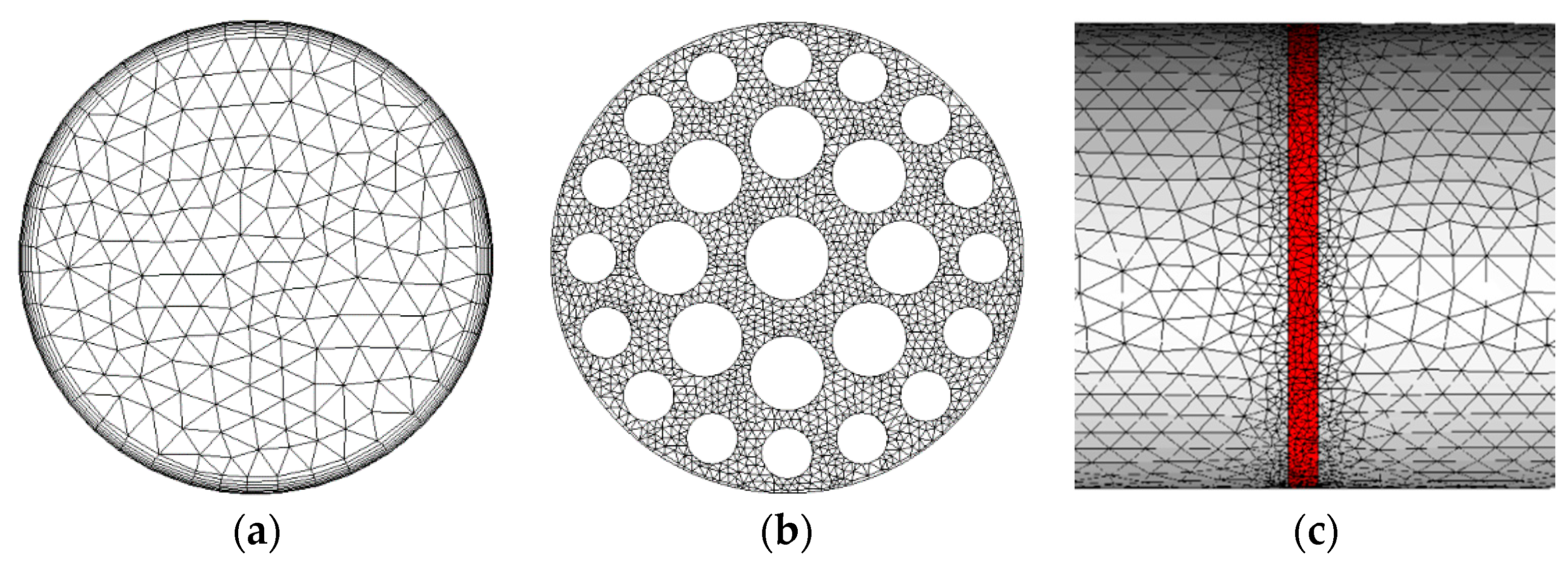
4.1. Geometric Modeling and Mesh Scheme

The geometric model used in the simulation was shown in Figure 10. The diameters of upstream and downstream header were both 200 mm, and the lengths were 2000 mm. There was a 90° elbow at the entrance of the upstream header. The diameter of the experimental pipe was 100 mm, while the length was 3500 mm.

The structure of FC was shown in Figure 11. It was installed at 100 mm downstream the header.

ANSYS-ICEM was employed to perform all geometry generation and meshing. Unstructured tetrahedron meshes were used to ensure the quality of the grid. The maximum size of the global grid was set as 15 mm, and the maximum size of all the surface grid was set as 8 mm. An exponential growth row on the surface to guarantee the sufficient near-wall mesh resolution was implemented to improve the prediction accuracy: the initial height was 0.05 mm, the height ratio was 1.3, and the number of layers was 10, as shown in Figure 12a. The grid density at the FC had been greatly increased, and the maximum grid size was 1, which was much smaller than the size of holes of the FC, as shown in Figure 12b. Moreover, the grid at the connection region near the FC was transitioned through gradual refinement (Figure 12c). A suitable grid density was reached by repeating computations until a satisfactory independent grid was found. The total number of grids for the entire model was about 5.7 million.

4.2. The Mathematical Method

The simulation parameters were based on actual experimental values of the gas flow standard device: the medium was air with the pressure 360 kPa, while the air was treated as the incompressible flow [25,31]. The air density was 4.2 kg/m³, and viscosity was 1.81 × 10⁻⁵ kg/(m·s). The five flow rate points selected in experiments of SN device were 2.9, 5.6, 7.6, 10.7, and 15.1 m/s, while they were 1, 5, 10, and 15 m/s, respectively with the Reynolds numbers 2.3 × 10⁴, 1.1 × 10⁵, 2.3 × 10⁵, and 3.5 × 10⁵ corresponding to the four flow points in simulation. So, all the conditions of flow were within the turbulence region.

The governing equations were represented by the conservation of mass and momentum, which were averaged using the well-known procedure introduced by Reynolds [44]. The Reynolds averaged Navier–Stokes k-ε turbulence model was one of the most widely used models in the turbulence simulation due to its high stability, economy, and accuracy. Compared with the standard k-ε model, the Renormalization-group (RNG) k-ε model could better respond to the influence of transient flow and streamline bending, and the model had better performance for a low Reynolds number and near-wall flow. So, the RNG k-ε turbulence model was adopted. Since steady-state incompressible flow was considered in this work, the RANS equations could be written as:

➢

mass conservation

$$\nabla \cdot \mathrm{U}=0$$

(6)

➢

momentum conservation

$$\nabla \cdot (\mathrm{U}\otimes \mathrm{U})=-\frac{1}{\rho }\nabla p+\nabla \cdot 2\mu \mathrm{D}-\nabla \cdot \mathrm{R}$$

(7)

where $\mathrm{U}=\left[\mathrm{U},\mathrm{V},\mathrm{W}\right]$ was the average velocity vector, $\mathrm{D}=\frac{1}{2}\left(\nabla \mathrm{U}+\nabla {\mathrm{U}}^T\right)$, and $\mathrm{R}=\left(\overline{\mathrm{u}\prime \otimes \mathrm{u}\prime }\right)$ represented the well-known turbulent or Reynolds stress tensor, due to fluctuating velocities $\mathrm{u}\prime =\left[u\prime ,v\prime ,w\prime \right]$.

The RANS k-ε model was found to give satisfactory results for the simulation of low-level disturbance and some flow conditioners [31,45,46].

4.3. Boundary Conditions

For all the problems studied, the following boundary conditions were assumed: the inlet boundary condition was “velocity-inlet”, the outlet boundary condition was “outflow”, and the wall boundary condition was default.

➢

walls

$$U=0,W=0,V=0$$

(8)

➢

inlet

$$U=U_0\frac{(n+1)\cdot (2n+1)}{2n^2}{\left(1-\frac{\sqrt{{(x+y)}^2}}{D}\right)}^{\frac{1}{n}},V=0,W=0$$

(9)

$$k=\frac{3}{2}{\left[U_m\cdot 0.16{\left(\mathrm{Re}\right)}^{-\frac{1}{8}}\right]}^2,\epsilon =0.164\frac{k^{\frac{3}{2}}}{0.07D}$$

(10)

➢

outlet

$$\frac{\partial }{\partial z}\left(U,V,W\right)=0$$

(11)

where n was the well-known function of Reynolds number, while k and ε could be evaluated from the turbulent intensity and length scale. For the simulation of a viscous layer near the walls, simplified models were used as well as the standard wall functions, in which a velocity profile was assumed on the basis of well-known empirical relations. The equations for the turbulent flow were solved outside this layer [46].

The code adopted for the numerical solution of the problem described above was based on the finite volumes technique. Finite volumes allowed, respectively to traditional finite difference schemes, modeling of complex geometry by using unstructured grids [46].

The discretized algebraic equations obtained from the finite volume procedure were solved using a semi-implicit algorithm, SIMPLEC, which was derived from that originally devised by Patankar [47]. The second-order up-winding scheme was used for all velocity terms in the momentum equation, and second-order interpolation was also used for pressure.

5. Analysis of Simulation Results

Based on the above CFD simulation, the detailed velocity information for each path could be obtained, which was used to analyze the flow distribution with different installation conditions.

For path i, the mean axial velocity components were given by Equation (12):

$${\overline{V}}_{xi}=\frac{1}{L_i}{\displaystyle {\int }_a^b{v}_{xi}\mathrm{d}L}\hspace{1em}{\overline{V}}_{yi}=\frac{1}{L_i}{\displaystyle {\int }_a^b{v}_{yi}\mathrm{d}L}\hspace{1em}{\overline{V}}_{zi}=\frac{1}{L_i}{\displaystyle {\int }_a^b{v}_{zi}\mathrm{d}L}$$

(12)

where L_i was the length of path i, v_xi, v_yi, and v_zi were instantaneous velocity components along the path, and V_xi, V_yi, and V_zi were the corresponding mean axial velocity components. Since the paths were arranged in parallel and perpendicular to the z-axis, the V_z did not contribute to the detected velocity along each path. Therefore, the average velocity along path i could be obtained by Equation (13) [22]:

$$V_i={\overline{V}}_{xi}+{\overline{V}}_{yi}\frac{\cos \beta }{\cos \phi }.$$

(13)

Here, based on the Cartesian coordinate system, the X-velocity component v_x and Y-velocity component v_y were selected to report the velocity profiles, as shown in Figure 13.

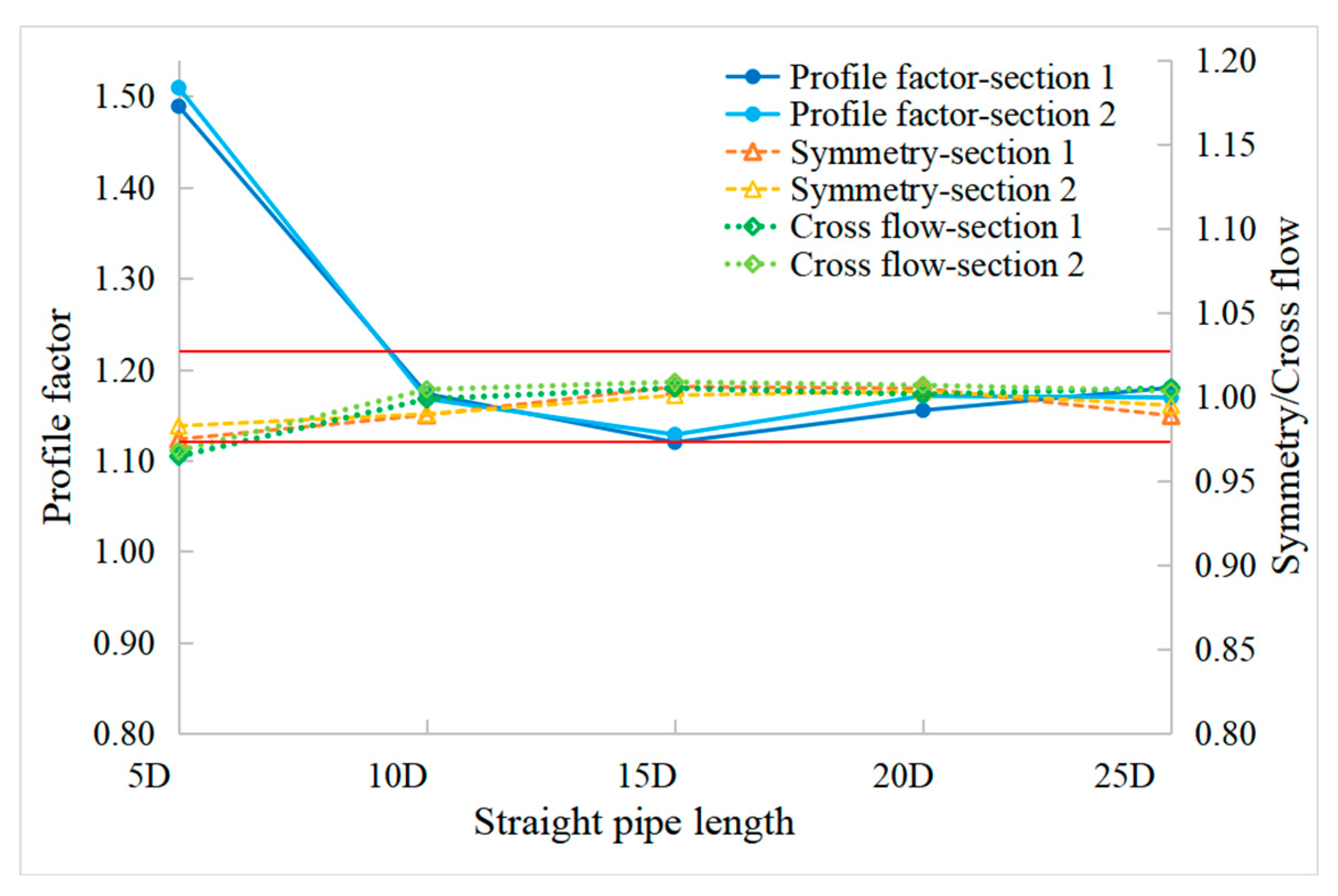
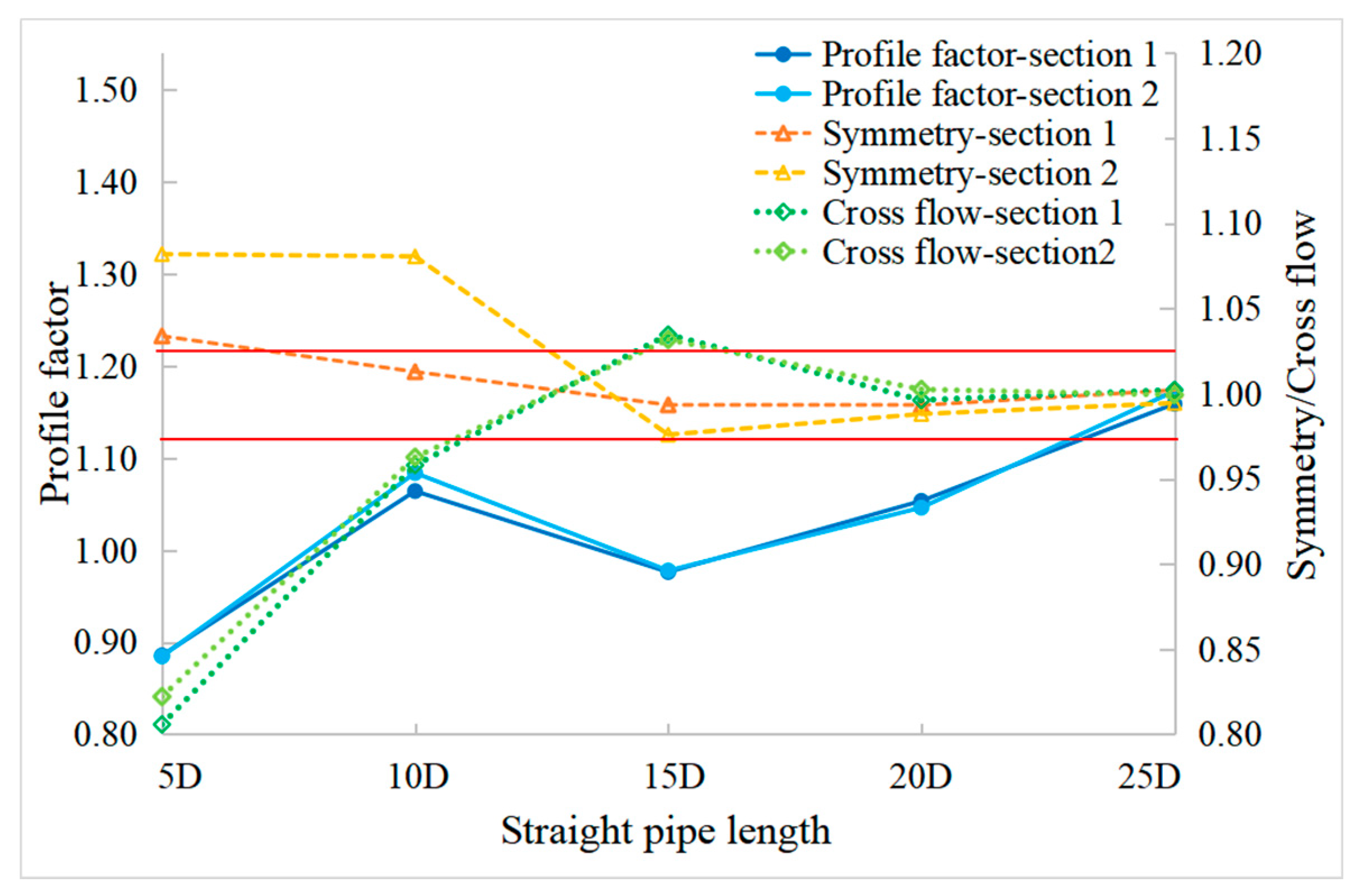
5.1. Velocity Distribution at Different Cross Sections

In order to visualize the flow field distribution, the velocity profile with the maximum velocity 15 m/s was analyzed.

By comparing the velocity distribution located at different cross-sections of the pipe from 5D to 25D downstream the header without FC, it showed that the velocity profile at 25D was nearly fully developed (Figure 14). Compared with it, the velocity profile changes obviously from 5D to 20D, and it gradually stabilized as the length of the straight pipe section increased. The larger the v_y was, the greater the distortion effect on measurement accuracy. It also showed the range of change in v_y.

One can see from Figure 15 that the velocity distributions on individual paths were of significant differences on different paths in the two sections at 10D without FC. Affected by the vortex, the velocity profile was obviously deformed, the velocities of v_B and v_C were decreased, and the velocities of v_A and v_D were increased. It reached a completely symmetrical distribution state at 25D.

From Figure 16, it can be seen that after the FC was installed, the high velocity began to converge toward the pipeline axis, the fluctuation of the velocity profile had been improved, and the maximum v_y did not exceed ±0.5 m/s even at 5D with FC.

Figure 17 showed that the velocity profile at 10D had been improved to some extent, and the flow distribution reached a fully developed state at about 15D. Thus, it could be found that the installation of FC could significantly improve the velocity profile and effectively eliminate swirls.

5.2. Analysis of Characteristic Parameters

The change of characteristic parameters with the increase of the straight pipe length under different installation conditions is shown in Figure 18 and Figure 19.

The Profile factor decreased with the straight pipe length increasing and met the requirements at about 10D with FC. The Symmetry and Cross-flow were close to 1 and kept relatively stable at about 10D, and there was no obvious difference between the two sections (Figure 18). Combined with Figure 16, the v_x of path B and C increased, and v_x of path A and D decreased, resulting in a Profile factor that was as high as 1.5 at 5D.

However, without FC, the Profile factor increased with the straight pipe length and met the requirements at about 25D. The Symmetry and Cross-flow varied dramatically at different positions, and the value could be acceptable at about 20D. In addition, the Symmetry were obvious different in the two sections (Figure 19). Combining Figure 14 with Figure 17, it was clear that the swirl occurred in the experimental pipe section (as shown in Figure 10) due to the header effect. The characteristic parameters were significantly affected by the swirl. When the FC was installed, all the values of the above three characteristic parameters could be acceptable at about 10D.

The variation of characteristic parameters at 19D corresponding to the experimental condition with the increase of Reynolds number or velocity is shown Figure 20. The Profile factor at 1 m/s was above the maximum allowable value both with or without FC. This was because the boundary layer effect was significant during the simulation process, which resulted in a lower velocity near the pipe wall, leading to the higher Profile factor. With FC, all the characteristic parameters met the requirements from 5 to 15 m/s. Nevertheless, the Symmetry and Cross-flow changed a little with the increasing of Reynolds number without FC, while the Profile factor dropped sharply, indicating that the effect of flow distortion was more significant with the increase of Reynolds number.

When the FC was not installed, the values of the Symmetry and Cross-flow were acceptable, while the value of the Profile factor was not. So, the difference occurred with different installation condition, which was consistent very well with the experimental results. It was proved again that Profile factor was an important indicator to characterize the velocity distribution.

6. Conclusions

In summary, by comparing the different results of the CL device and SN device under three different installation conditions, the influence of the flow field distortion generated by the header on the USM measurement results was studied. Based on the experimental results, the flow field distribution was further investigated by CFD simulation. The main conclusions were as follows:

➢

The accurate experimental results showed that the measurement results of SN device were consistent very well with the CL device, while the measurement error of the SN device without FC was about 1% higher than the reference. The flow field distortion effect generated by the header had a significant influence on the measurement results of USM due to the nonconforming Profile factor, while the difference of Symmetry and Cross-flow could be obviously eliminated by the double-cross-section designing;

➢

The simulation results showed that it was at about 25D without FC in the SN device that the velocity profile restored to a fully developed state and all characteristic parameters could meet the requirements, while it was at 10D with FC. The installation of FC could improve the accuracy of measurement results, because the FC could improve the velocity profile, and it also could effectively eliminate vortices and cross-flow.

The characteristic parameter of USM could be determined when the meter was calibrated in the laboratory. When the USM was used in the field with header, these values should be checked to ensure that the field installation was satisfactory in terms of flow field distribution. Once installed, they can be checked again periodically. Any significant change in these parameters that does not correlate with a change in Re or upstream pipework should be investigated further.

References

1. Brown, G.J.; Augenstein, D.R.; Cousins, T. An 8-Path Ultrasonic Master Meter for Oil Custody Transfers. In Proceedings of the XVIII IMEKO World Congress, Rio de Janeiro, Brazil, 17–22 September 2006. [Google Scholar]
2. Lynnworth, L.C.; Liu, Y. Ultrasonic flowmeters: Half-century progress report, 1955–2005. Ultrasonics 2006, 44, e1371–e1378. [Google Scholar] [CrossRef] [PubMed]
3. Drenthen, J.G.; Boer, G.D. The manufacturing of ultrasonic gas flow meters. Flow Meas. Instrum. 2002, 12, 89–99. [Google Scholar]
4. Nabavi, M.; Siddiqui, K. A critical review on advanced velocity measurement techniques in pulsating flows. Meas. Sci. Technol. 2010, 21, 042002. [Google Scholar] [CrossRef]
5. Zhou, A.G.; Ruan, J.Y.; Liu, K.; Lu, M.X. Analysis and strategy for impacts on ultrasonic flowmeters. Chin. J. Construct. Mach. 2009, 7, 469–473. [Google Scholar]
6. Lin, Q.; Chen, Z.X.; Zhang, Y.Y.; Xiao, Q.; Yang, Z.Y.; Bai, X.F. Overview of ultrasonic flowmeter and numerical simulation of flow field. Tech. Superv. Petro Ind. 2018, 34, 43–47. [Google Scholar]
7. Rundle, J.B. Viscoelastic crustal deformation by finite quasi-static sources. J. Geophys. Res. Solid Earth Planets 1978, 83, 5937–5945. [Google Scholar] [CrossRef]
8. Mousavi, S.F.; Hashemabadi, S.H.; Jamali, J. Calculation of Geometric Flow Profile Correction Factor for Ultrasonic Flow Meter Using Semi-3D Simulation Technique. Ultrasonics 2020, 106, 106165. [Google Scholar] [CrossRef] [PubMed]
9. Zhou, H.L.; Ji, T.; Wang, R.C.; Ge, X.; Tang, X.; Tang, S. Multipath ultrasonic gas flow-meter based on multiple reference waves. Ultrasonics 2017, 82, 145–152. [Google Scholar] [CrossRef] [Green Version]
10. Lansing, J.; Herrmann, V.; Dietz, T. Investigations on an 8 path ultrasonic meter-What sensitivity ro upstream disturbance remain? In Proceedings of the 24th International North Sea Flow Measurment Workshop, St. Andrews, UK, 24–27 October 2006. [Google Scholar]
11. Zhao, H.C.; Peng, L.H.; Tsuyoshi, T.; Hayashi, T.; Shimizu, K.; Yamamoto, T. ANN Based Data Integration for Multi-Path Ultrasonic Flowmeter. IEEE Sens. J. 2013, 14, 362–370. [Google Scholar] [CrossRef]
12. Zheng, D.D.; Zhao, D.; Mei, J.Q. Improved numerical integration method for flowrate of ultrasonic flowmeter based on Gauss quadrature for non-ideal flow fields. Flow Meas. Instrum. 2015, 41, 28–35. [Google Scholar] [CrossRef]
13. Wang, B.; Cui, Y.; Liu, W.; Luo, X. Study of Transducer Installation Effects on Ultrasonic Flow Metering Using Computational Fluid Dynamics. Adv. Mater. Res. 2013, 629, 676–681. [Google Scholar] [CrossRef]
14. Chen, W.G. Analysis and Compensation Method of Non-Ideal Flow Field for Ultrasonic Gas Flowmeter. Ph.D. Thesis, Zhejiang University, Hangzhou, China, 2015. [Google Scholar]
15. Heinig, D.; Wenzel, J.; Nerowski, D.A.; Dietz, T. An Innovative Approach to Increase Diagnostic Sensitivity in Ultrasonic Flow Meters. In Proceedings of the 36th North Sea Flow Measurement Workshop, Tønsberg, Norway, 22–25 October 2018. [Google Scholar]
16. Hallanger, A.; Saetre, C.; Frøysa, K.E. Flow profile effects due to pipe geometry in an export gas metering station—Analysis by CFD simulations. Flow Meas. Instrum. 2018, 61, 56–65. [Google Scholar] [CrossRef]
17. American Gas Association. Measurement of Gas by Multipath Ultrasonic Meters; Report No. 9; AGA: Washington, DC, USA, 1998. [Google Scholar]
18. Qin, L.H.; Hu, L.; Mao, K.; Chen, W.; Fu, X. Flow profile identification with multipath transducers. Flow Meas. Instrum. 2016, 52, 148–156. [Google Scholar] [CrossRef]
19. Measurement of Natural Gas Flow by Gas Ultrasonic Flow Meters; GB/T 18604-2014, ICS 75.180.30; China Standards Press: Beijing, China, 2014.
20. Matiko, F.; Roman, V.; Baitsar, R. Methodology for Improving Mathematical Model of Ultrasonic Flowmeter to Study Its Error at Distorted Flow Structure. Energy Eng. Control Syst. 2015, 1, 63–70. [Google Scholar]
21. Mickan, B.; Wendt, G.; Kramer, R.; Dopheide, D. Systematic investigation of flow profiles in pipes and their effects on gas meter behaviour. Measurement 1997, 22, 1–14. [Google Scholar] [CrossRef]
22. Zheng, D.D.; Zhang, P.Y.; Xu, T.S. Study of acoustic transducer protrusion and recess effects on ultrasonic flowmeter measurement by numerical simulation. Flow Meas. Instrum. 2011, 22, 488–493. [Google Scholar] [CrossRef]
23. Ruppel, C.; Peters, F. Effects of upstream installations on the reading of an ultrasonic flowmeter. Flow Meas. Instrum. 2004, 15, 167–177. [Google Scholar] [CrossRef]
24. Leontidis, V.; Cuvier, C.; Caignaert, G.; Dupont, P.; Roussette, O.; Fammery, S.; Nivet, P.; Dazin, A. Experimental validation of an ultrasonic flowmeter for unsteady flows application. Meas. Sci. Technol. 2018, 29, 1–17. [Google Scholar] [CrossRef] [Green Version]
25. Sætre, C.; Frøysa, K.-E.; Hallanger, A.; Chan, P. Installation effects and flow instabilities in gas metering station with multipath ultrasonic flow meters. In Proceedings of the 33rd International North Sea Flow Measurement Workshop, Tonsberg, Norwey, 20–23 October 2015. [Google Scholar]
26. Zhu, W.J.; Xu, K.J.; Fang, M.; Wang, W.; She, Z.-W. Mathematical Modeling of Ultrasonic Gas Flow Meter Based on Experimental Data in Three Steps. IEEE Trans. Instrum. Meas. 2016, 65, 1726–1738. [Google Scholar] [CrossRef]
27. Liu, E.B.; Tan, H.; Peng, S.B. A CFD simulation for the ultrasonic flow meter with a header. Teh. Vjesn. Tech. Gaz. 2017, 24, 1797–1801. [Google Scholar]
28. Zheng, D.D.; Lv, S.H.; Mao, Y. Effect mechanism of non-ideal flow field on acoustic field in gas ultrasonic flowmeter. IET Sci. Meas. Technol. 2019, 13, 469–477. [Google Scholar] [CrossRef]
29. Johnson, A.N.; Boyd, J.T.; Harman, E.; Khail, M.; Ricker, J.R.; Crowley, C.J.; Wright, J.D.; Bryant, R.; Shinder, I. Design and Capabilities of NISTs Scale-Model Smokestack Simulator (SMSS). In Proceedings of the 9th International Symposium on Fluid Flow Measurement, Arlington, VA, USA, 14–17 April 2015. [Google Scholar]
30. Zhang, H.; Guo, C.W.; Lin, J. Effects of Velocity Profiles on Measuring Accuracy of Transit-Time Ultrasonic Flowmete. Appl. Sci. 2019, 9, 1648. [Google Scholar] [CrossRef] [Green Version]
31. Zhao, H.C.; Peng, L.H.; Stephane, S.A.; Ishikawa, H. CFD Aided Investigation of Multipath Ultrasonic Gas Flow Meter Performance under Complex Flow Profile. IEEE Sens. J. 2014, 14, 897–907. [Google Scholar] [CrossRef]
32. Hallanger, A.; Frøysa, K.E.; Lunde, P. CFD-simulation and installation effects for ultrasonic flow meters in pipes with bends. Int. J. Appl. Mech. Eng. 2002, 7, 33–64. [Google Scholar]
33. Yao, P. Measurement Accuracy Improvement Method of Gas Ultrasonic Flowmeter in Complex Flow Field. Master’s Thesis, Zhejiang University, Hangzhou, China, 2018. [Google Scholar]
34. Zhu, W.J.; Xu, K.J.; Fang, M.; Shen, Z.-W.; Tian, L. Variable ratio threshold and zero-crossing detection based signal processing method for ultrasonic gas flow meter. Measurement 2017, 103, 343–352. [Google Scholar] [CrossRef]
35. ASME PTC18-2011_Hydraulic Turbines and Pump-Turbines Performance Test Codes; The American Society of Mechanical Engineers: New York, NY, USA, 2011.
36. Grunert, F.; Kabra, Z. Effect of symmetric distortion of the field of fluid velocity on the readings of an ultrasonic flowmeter. Meas. Tech. 1997, 40, 445–451. [Google Scholar] [CrossRef]
37. Li, C.H.; Mickan, B.; Cui, L.S. The high pressure sonic nozzle gas flow standard facility in NIM. In Proceedings of the Flomeko 2019, Lisbon, Portugal, 26–28 June 2019. [Google Scholar]
38. Wang, C.; Li, C.H.; Xu, M.; Yan, W. The high pressure close loop gas flow standard facility in NIM. In Proceedings of the Flomeko 2019, Lisbon, Portugal, 26–28 June 2019. [Google Scholar]
39. Hoffmann, B.H. Path Following and Collision Avoidance for an Underwater Swimming Manipulator. Master’s Thesis, Norwegian University of Science and Technology, Trondheim, Norway, 2018. [Google Scholar]
40. Chun, S.; Yoon, B.R.; Lee, D.K.; Choi, H.-M. Correction of flow metering coefficients by using multi-dimensional non-linear curve fitting. J. Mech. Sci. Tech. 2012, 26, 3479–3489. [Google Scholar] [CrossRef]
41. Lindsay, G. Review of NEL’s Ingernal Knowledge in the Field of Flow Meter Diagnostics; National Engineering Laboratory: East Kilbride, UK, 2019. [Google Scholar]
42. Emerson Process Management; Daniel Measurement and Control, Inc. How Today’s Ultrasonic Meter Diagnostics Solve Metering Problems Technical White Paper; Daniel Measurement and Control, Inc.: Houston, TX, USA, 2010. [Google Scholar]
43. Gallagher, J.E. Natural Gas Measurement Handbook; Elsevier: Amsterdam, The Netherlands, 2007; Chapter 4; pp. 79–110. [Google Scholar]
44. Schlichting, H.; Gersten, K. Boundary-Layer Theory; Springer: Berlin/Heidelberg, Germany, 1979; ISBN 978-3540662709. [Google Scholar]
45. Erdal, A. A numerical investigation of different parameters that affect the performance of a flow conditioner. Flow Meas. Instrum. 1998, 8, 93–102. [Google Scholar] [CrossRef]
46. Frattolillo, A.; Massarotti, N. Flow conditioners efficiency a comparison based on numerical approach. Flow Meas. Instrum. 2002, 13, 1–11. [Google Scholar] [CrossRef]
47. Patankar, S.V. Numerical Heat Transfer and Fluid Flow; CRC Press: Boca Raton, FL, USA, 1 January 1980; 214p, ISBN 9780891165224. [Google Scholar]
Figure 1. Working principle of transit-time multipath ultrasonic flowmeter (TM-USM).
Applsci 11 03656 g001
Figure 2. Schematic of a 2-section/8-path TM-USM (a) top view, (b) side view, (c) stereo schematic.
Applsci 11 03656 g002
Figure 3. Schematic diagram of the sonic nozzle secondary standard device.
Applsci 11 03656 g003
Figure 4. Schematic diagram of the close loop working standard device.
Applsci 11 03656 g004
Figure 5. The flow conditioner.
Applsci 11 03656 g005
Figure 6. Results with different installation conditions at 0.36 MPa.
Applsci 11 03656 g006
Figure 7. The difference between two devices at different pressures.
Applsci 11 03656 g007
Figure 8. The characteristic parameters of flow distribution in different sections. (a) Without flow conditioner (FC), (b) With FC.
Applsci 11 03656 g008
Figure 9. The difference between the parameters with different installation conditions.
Applsci 11 03656 g009
Figure 10. Schematic diagram of computational fluid dynamics (CFD) model.
Applsci 11 03656 g010
Figure 11. Diagram of plate flow conditioner.
Applsci 11 03656 g011
Figure 12. The grid in the vicinity of the FC and boundary layer. (a) The boundary layer grid; (b) The greatly increased grid of FC; (c) Grid at the connection region near FC.
Applsci 11 03656 g012
Figure 13. The orientation of the velocity components in the pipe.
Applsci 11 03656 g013
Figure 14. Contours of velocity profiles on the different cross-sections downstream of the header without FC.
Applsci 11 03656 g014
Figure 15. Velocity distribution on individual paths without FC. (a) 10D; (b) 25D.
Applsci 11 03656 g015
Figure 16. Contours of velocity profiles on the different cross-sections downstream of the header with FC.
Applsci 11 03656 g016
Figure 17. Velocity distributions on individual paths with FC. (a) 10D; (b) 15D.
Applsci 11 03656 g017
Figure 18. Characteristic parameters with FC.
Applsci 11 03656 g018
Figure 19. Characteristic parameters without FC.
Applsci 11 03656 g019
Figure 20. Characteristic parameters at 19D corresponding to the experimental condition.
Applsci 11 03656 g020