Abstract
This work investigates the possibility of applying Fourier Transform (FT) analysis of the force signal to follow fatigue behavior of metals under oscillatory displacement-controlled tests in uniaxial tension/tension. As a first step, three different materials were selected (cold rolled steel, aluminium and brass). The FT analysis revealed a low level of nonlinearities in the force response, which was possible to measure and quantify as higher harmonics of the imposed sinusoidal deformation. Due to geometric reasons, the odd higher harmonics represent the symmetric nonlinearity while even ones are related to asymmetry, so both odd and even harmonics need to be analyzed separately. The time evolution of the higher harmonics showed that the odd higher harmonics continuously increase during the test. Criteria to better predict the mechanical fatigue and failure (life time) are then proposed based on the integral and derivative based on the time evolution the odd higher harmonics. In contrast, for tests in the high cycle fatigue regime, the even higher harmonics are mainly noise at the beginning of the test (undamaged state), but start to rise after the occurrence of a crack due to internal crack friction. Based on the analysis performed, FT analysis of the force during mechanical fatigue testing of metals is a sensitive tool used to predict failure and to improve our understanding of the dynamics involved in mechanical fatigue.
1. Introduction
1.1. Mechanical Fatigue of Metals
Failure of a part under a repetitive load is called mechanical fatigue break-up. Even today, the most common and straightforward way to investigate mechanical fatigue is to identify a correlation between the number of cycles to failure (Nf) with the average applied stress (σ0) or the strain amplitude (ε0) for stress or strain controlled tests respectively; i.e., the so-called S-N or strain-life curves [1]. In the stress or strain controlled mode, a power-law relation between Nf and the global average stress/strain amplitude is typically observed. In the high cycle fatigue regime, the equation is:
where AStrain-life and a are the prefactor and the exponent of the strain-life curve, respectively.
Strain-life curves report the average value of the number of cycles necessary for part failure under specific loading conditions over a certain amount of fatigue tests for the same testing conditions. Consequently, they only provide information about the most probable number of cycles to failure [2], but no information about the failure process (onset of cracks). In general, reproducibility of the fatigue lifetime under the same measurement conditions is poor, so a wide span of lifetimes is typically measured resulting in high standard deviations [3]. Typically, two orders of magnitude are commonly reported for notched as well as smooth specimens [4]. A more precise prediction is difficult due to the probabilistic nature of mechanical fatigue [5].
The combination of long testing times and high experimental uncertainties make fatigue testing time and resources intensive. Consequently, the predictive power of a measured fatigue lifetime for a single sample or application is very limited. This is why a deeper understanding of the fatigue process is needed, not only to predict and avoid failure (accidents), but also to save resources by not stopping the test/application too early due to high safety factors.
For metallic materials, different techniques and concepts have been developed to better describe and understand the fatigue process, as well as to predict failure more precisely. Experimental concepts are based on heat dissipation due to plastic deformation [6,7], via metal magnetic memory (MMM) [8], or by following the electrical conductivity [9].
Experimental techniques to quantify nonlinear material behavior have been used, such as ultrasonic techniques to detect nonlinear material behavior. These techniques successfully showed that the nonlinear material properties change due to fatigue [10,11]. So the objective of this work was to expand these techniques by analyzing the stress response via Fourier transform of metallic specimens in displacement-controlled fatigue tests. From the results obtained, better fatigue life times are predicted, as well as the possibility to easily detect crack initiation and propagation with high sensitivity.
1.2. Nonlinear Material Behavior during Fatigue
When a sample is deformed in cyclic strain controlled tension/tension (T/T), the constant static deformation is larger than the strain amplitude (ε0) of the dynamic deformation, to avoid compression at the strain minimum of each cycle. The ratio between the minimum (εmin) and maximum (εmax) deformation is described by the deformation ratio (R) and correlates with ε0 as [1]:
The oscillatory time dependent elongational strain ε(t) can be described by a simplified complex notation as:
which can be decomposed into a static (εs) and a dynamic (εd*) part.
In our previous works, a framework was established to quantify the mechanical nonlinear material behavior of polymers via Fourier transform of the stress response in strain controlled testing. The developed concepts are explained as follows. Under strain controlled sinusoidal testing, the stress response of polymers becomes nonlinear under sufficiently large amplitude oscillatory elongation (LAOE) [12]. Nonlinearity means in this context, that the stress response and the applied strain are not directly proportional to each other, so the linear material parameters such as storage (E′) and loss (E″) moduli loose their physical meaning as material parameters. Fourier transform is a very powerful tool to detect nonlinear contributions, as well as to analyze and quantify the resulting (nonlinear) stress waveform with very high sensitivity [12,13]. This is done by analyzing the higher harmonics of the Fourier spectra in the frequency domain of the time dependent stress. For a sufficiently high number of data points in the time domain, the stress can be quantified in the frequency domain using a limited number of frequency at multiples of the fundamental frequency as I(), I(2), I(3), etc., while the remaining points of the spectra are considered as non-periodic and are assumed as noise as a first approximation [14,15]. In this case, the harmonics analysis acts as a very efficient filter of the time data using σ(t) = σ(t + T) where T is the period time.
For a periodic nonlinear asymmetric stress response, either caused by the loading conditions [16] or specimen anisotropy [17], the stress and the moduli depend on the deformation direction so σ*(t)(ε+) − σmean ≠ −(σ*(t)(ε−) − σmean) or E′(t)(ε+) ≠ E′(t)(ε−) and E″(t)(ε+) ≠ E″(t)(ε−). Consequently, the modulus becomes a function of the applied deformation as E* = E(ε*) and a Taylor series expansion of the strain dependent modulus can be developed containing both even and odd powers of the strain as [18]:
The stress response of the simplest nonlinear 1D scalar model for an elastic solid body (spring) can be described by Hooke’s law as:
Inserting Equation (3) into Equation (5) and simplifying the notation gives:
In general, for viscoelastic materials, Equation (6) can be rewritten including phase angles to show that an asymmetric nonlinear stress response includes a constant value and a fundamental harmonic, as well as even and odd higher harmonics as [12,18,19]:
A nonlinear, but symmetric, stress response occurs if the stress response is independent of the deformation direction; i.e., it is similar during loading and unloading: σ*(t)(ε+) − σmean = −(σ*(t)(ε−) − σmean). In this case, the Taylor series of the stress only contains odd higher harmonics due to geometrical symmetry arguments, underlining the different geometric meanings of the even and odd higher harmonics [12]. This is why both contributions need to be analyzed separately to understand the physical origin of mechanical nonlinearity.
The magnitude of the generated higher harmonics (In, n > 1) are typically normalized by the fundamental (I1) as In/I1 = In/1. For example, the relative third harmonic intensity is presented as I3/1. Equation (6) shows that the normalized intensities of the higher harmonics should scale as power-law functions of ε0 with exponents of n − 1 [20]. For example, I2/1 and I3/1 should scale linearly and quadratically with respect to ε0. This was experimentally observed and mathematically derived for several materials [20,21,22,23].
To quantify the materials nonlinearity while being independent of the measurement conditions, and to obtain a nonlinear material parameter, the proportionality factor between I3/1 and ε0 is defined as the Q parameter [20,22]:
In a strain controlled fatigue test, the applied strain amplitude (ε0), as well as the angular frequency (ω1), are constant, while the stress response changes due to ongoing fatigue [24]. On the one hand, the stress amplitude decreases and its nonlinearity (deviation from a sinusoidal waveform with the fundamental frequency ω1) increases [25]. Both phenomena result in decreasing E′ and E″ combined with increasing mechanical nonlinearity quantified via the I3/1 intensity.
Recently, a framework was developed to analyze, quantify and predict the fatigue behavior via Fourier transform of the stress response by individually analyzing each higher harmonic for brittle polymers under T/T. Three concepts based on the higher harmonics were introduced: (I) the detection of macroscopic cracks via the I2/1 intensity [19], (II) the prediction of fatigue failure via the rate of change of the I3/1 intensity [26], and (III) the cumulative nonlinearity Qf as a fatigue criterion [27]. With ongoing fatigue, the nonlinear mechanical parameter (I3/1 and Q) were found to monotonously increase for rectangular notched and unnotched samples [26,27].
Based on previous results, it was found that during testing I3/1 goes through three different regimes until failure. At the beginning of the test (regime I), a transient period was found with a fast increase (dI3/1/dN ≠ const.), followed by a linear increase with the cycle number in regime II (dI3/1/dN = const.) leading to failure onset in regime III when I3/1 increases rapidly. The fatigue lifetime (Nf) was found to be inversely proportional to the rate of change of I3/1 (dI3/1/dN) in regime II as:
Equation (9) was shown to have a much lower deviation (±30%) compared to standard strain-life curves (span of Nf of a factor of 3–4), with the proportionality factor AI3/1 being polymer specific [26].
Furthermore, a nonlinear fatigue criterion was developed based on the cumulative nonlinearity (Qf) which represents the integral of the nonlinearity (Q) from the beginning of the test until failure [27]:
Similar fatigue criteria exist for lifetime prediction like the cumulative strain energy density [28], or the cumulative dissipated energy density [29]. Above the very low cycle fatigue regime a power-law correlation between Qf and Nf was found as:
where AQ is the proportionality constant.
Due to the poor reproducibility of mechanical fatigue, the developed concepts are widely applicable from a high-sensitive support tool for material testing in fundamental research to the development of smart surveillance systems (sensors) for mechanical fatigue in construction and transportation applications. Additionally, the detection via I2/1 is not limited to viscoelastic materials, as it changes after the occurrence of a macroscopic crack due to an asymmetry in the stress response [19]. Therefore, its value/trend can be used not only for the detection of cracks in materials or applications, which cannot be detected from the outside, but also represents a non-destructive parameter for the detection of voids or defects from the manufacturing process.
From our previous work on polymers, it was concluded that FT analysis of the stress is a powerful tool as the I2/1 intensity can be used to detect the onset of cracks and I3/1 to predict the fatigue lifetime. So, the main objective of this work was to apply the technique of Fourier transform analysis of the stress response under fatigue testing on metallic specimens. By doing so, the idea is to determine if: (I) nonlinear material behavior occurs, (II) the nonlinear material behavior changes due to fatigue and (III) fatigue can be quantified by Fourier transform analysis.
2. Materials and Test Setup
Three type of metallic samples were selected for the experimental investigation: aluminum (AL 6061-T6, 97.2% Al, 1% Mg, 0.6% Si, 0.3% Cu, 0.3% Fe, 0.2% Cr, 0.2% Zn, 0.1% Mn, 0.1% Ti), cold rolled steel (CRS, 1018, 99% Fe, 0.8% Mn, 0.2% C) and brass (C36000, 61.5% Cu, 35.4% Zn, 2.7% Pb).
The dynamic tensile fatigue tests were performed with a sinusoidal deformation at a frequency of 5 Hz with R = 0.1 and a distance between grips of 24 mm on an Acumen 3 (MTS, Eden Prairie, MN, USA) mechanical tester in the strain controlled mode. The time signals for the force and deformation under dynamic testing were recorded via a custom written LabView program with a sampling rate of 200 points/cycle using oversampling [30]. Using a custom written MATLAB script, the nonlinear parameters (I2/1 and I3/1) were calculated via Fourier transform. The tests were performed at room temperature (RT ≈ 23 °C) and followed by a thermal camera (FLIR ThermoVision A320). More information on the experimental set-up and data analysis can be found in our previous works [19,21,26,31,32].
The fracture surface was investigated via microscopy (Olympus SZ-PT).
3. Tensile Tests
Firstly, tensile tests were performed on the materials at a strain rate of 3 mm/min. As it can be seen in Figure 1, CRS has the highest modulus and elongation at break, followed by brass and AL. Furthermore, only at very low strain (ε < 0.5%) are the stress and strain directly proportional to each other; i.e., the linear regime following Hooke’s law. At larger strains, the material response becomes nonlinear: the materials yield and break.
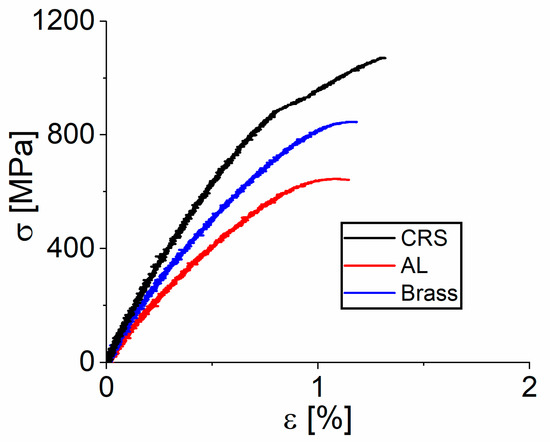
Figure 1.
Tensile stress-strain curve (3 mm/min) for CRS, AL and brass showing a nonlinear material behavior (deviation from Hooke’s law) above ε = 0.5%.
4. Fourier Spectrum
To investigate the mechanical nonlinear behavior of metallic specimens, cyclic tests were performed at a given strain amplitude and the force response was analyzed via FT. Figure 2 presents the FT spectra of the materials at ε0 = 0.4% (R = 0.1, εmax = 0.89%) and ω1/2π = 5 Hz. The spectra show a good signal to noise ratio in the range of 104:1, so that the measured higher harmonics can be seen as quantification of a nonlinear material response. Beside the fundamental harmonic at 5 Hz, the FT spectra show also higher harmonics at 10 Hz, 15 Hz, etc., clearly indicating nonlinear material behavior. It is interesting to note that the even higher harmonics, such as I2/1, I4/1, etc. (at 10 Hz, 20 Hz, etc.), have lower intensities as the odd ones I3/1, I5/1, etc. (15 Hz, 25 Hz, etc.), so the nonlinear symmetric contribution in the material response exceeds the nonlinear asymmetric one.
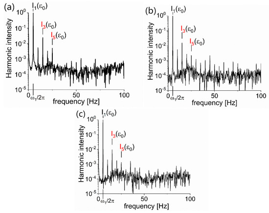
Figure 2.
Fourier spectrum of the force response for (a) AL, (b) CRS and (c) brass at a frequency of 5 Hz and a strain amplitude of ε0 = 0.16%.
5. Strain Sweep Behavior
To follow the dependence of the linear and nonlinear mechanical parameters on the applied strain, strain sweep tests were performed (the strain amplitude was changed, but R was kept constant). As shown in Figure 3, the three materials investigated show a |E*| decrease at strain amplitudes larger than ε0 = 0.04%. For ε0 < 0.04%, the intensities of the higher harmonics decrease with an exponent of around −1, as expected for experimental noise (motor and/or force transducer) and can be neglected, while the I3/1 intensity scales quadratically with ε0 above ε0 = 0.04% before leveling off. Additionally, the I2/1 intensity is always much lower than the I3/1 value.
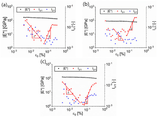
Figure 3.
Strain sweep tests for: (a) CRS, (b) AL and (c) brass. The plots report on the complex modulus |E*| and the nonlinear parameters (I2/1 and I3/1) as a function of the applied strain amplitude. While there is no trend for I2/1 (only noise), the I3/1 intensity scales quadratically with ε0 above ε0 = 0.7%.
6. Strain-Life Curves
In Figure 4 the strain-life curves of the materials investigated are presented. For the three materials, strain amplitude and fatigue lifetime follow a power-law correlation with exponents around −0.27 via:
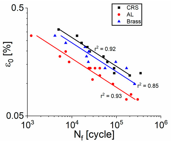
Figure 4.
Strain-life curves for CRS (black square), AL (red circle) and brass (blue triangle) revealing the poor reproducibility and prediction precision of this type of representation.
But a high scattering of the data points around the best fit is observed; i.e., the reproducibility under the same measurement conditions is low and may vary under the same measurement conditions by up to a factor of four. So, following the linear and nonlinear mechanical parameters as a function of the cycle number should give better prediction of the fatigue lifetime and better insights into the fatigue process.
7. Behavior of the Nonlinear Parameters during Fatigue
Figure 5 shows the evolution of the mechanical parameters |E*|, I2/1 and I3/1 as a function of the cycle number for a fatigue test using AL at ε0 = 0.08%. It can be seen that |E*| is strain hardening in the first few cycles of the test, then decreases until failure. But more importantly, the changes are less than 2% of the initial value for over 90% of the complete fatigue lifetime, before a sudden decrease occurs very close to failure. This lack of sensitivity (below the experimental uncertainty) indicates that |E*| is a poor criterion to predict a part’s failure needing high safety factors. On the contrary, the higher harmonics substantially change over the duration of the test. The first odd higher harmonic (I3/1) slightly decreases at first or stays constant which is associated to regime I. For the test presented in Figure 5 this is valid up to N = 30,000 cycles which represents 15% of its complete fatigue lifetime. Between N = 30,000 and N = 160,000 cycles, the I3/1 intensity increases with a constant slope (dI3/1/dN = const.) which is associated to regime II. Beyond N = 160,000 cycles, a rapid growth is observed leading to failure onset as regime III. This last part of the curve implies a 50% increase from the minimum value in regime I to failure in regime III. For the first even higher harmonic (I2/1), which represents the level of asymmetry in the force response, its value also changes with ongoing fatigue, but with lower intensity than for I3/1. At the beginning of the test, I2/1 is constant (noise level), but around N = 75,000 cycles, the value starts to slowly increase before a faster variation is observed, especially getting closer to failure. In this case, the change is by a factor of 20 compared to the initial constant value. In both cases (I2/1 and I3/1), the variation are much higher than |E*|, which does not change by more than 5% before failure. These sensitivity differences will be investigated in more details in the next section. In fact, the fast I2/1 increase can be associated to the onset of a macroscopic crack generating internal friction between the fractured surfaces.
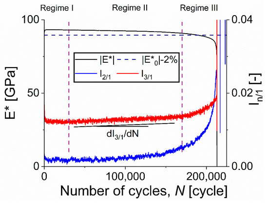
Figure 5.
The mechanical parameters (|E*|, I2/1 and I3/1) as a function of the cycle number (N) for an aluminum sample at ε0 = 0.08%, ω1/2π = 5 Hz and R = 0.1.
7.1. Crack Detection
As described before, the complex modulus is not a very sensitive parameter for the detection of a crack. After crack initiation, the newly created surfaces touch/compress each other as crack friction, resulting in an additional force, superposing with the material force response, so the force response of the material becomes asymmetric. If the stress signal is decomposed via FT, this leads to even higher harmonics, so the I2/1 intensity increases above the noise level (initial value). A similar behavior was observed for polymers in T/T [23,31].
As reported using logarithmic axes for the In/1, Figure 6, Figure 7 and Figure 8 show that the I2/1 intensity is constant (noise level) at the beginning of a test. Then, the I2/1 intensity increases at a specific time (crack initiation) until failure, after N = 75,000 and 90,000 in Figure 6, after N = 90,000 and 280,000 cycles in Figure 7 and after N = 220,000 and 45,000 cycles in Figure 8 respectively, as a larger crack will result in higher crack friction, i.e., an asymmetric force from the newly created crack surfaces. As a consequence, the force response between the strain maximum and strain minimum becomes asymmetric, which can be quantified by the even higher harmonics, in particular the I2/1 intensity. This can be observed for lower strain amplitudes and longer lifetimes, when crack growth is a significant part of the fatigue lifetime, thus crack propagation occurs before the sudden and complete brittle fracture when the material can no longer sustain the stress concentration at the crack tip.
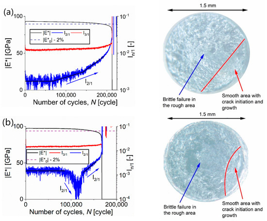
Figure 6.
Mechanical parameters (|E*|, I3/1 and I2/1) for a fatigue test of AL at ε0 = 0.08% (a) and ε0 = 0.072% (b) at 5 Hz, revealing a change of the I2/1 intensity from the noise level after N = 75,000 and 90,000 cycles, respectively. On the right side the fracture surface is presented, using 40× magnification, revealing a smooth and a rough surface area, correlating with crack initiation and brittle failure, respectively. Compared with the rough area, the smooth area is small matching with the very small |E*| change before failure.
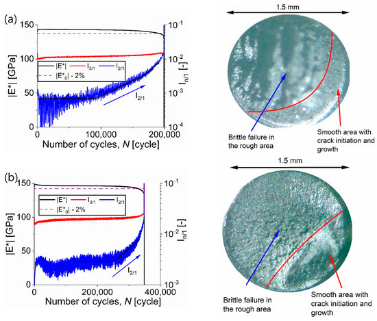
Figure 7.
Mechanical parameters (|E*|, I3/1 and I2/1) for a fatigue test of cold rolled steel at ε0 = 0.12% (a) and ε0 = 0.125% (b) at 5 Hz, revealing the increase of the I2/1 intensity above the noise level after N = 90,000 and 280,000 cycles, respectively. On the right side the fracture surface is presented, using 40× magnification, revealing a smooth and a rough surface area, correlating with crack initiation and brittle failure, respectively.
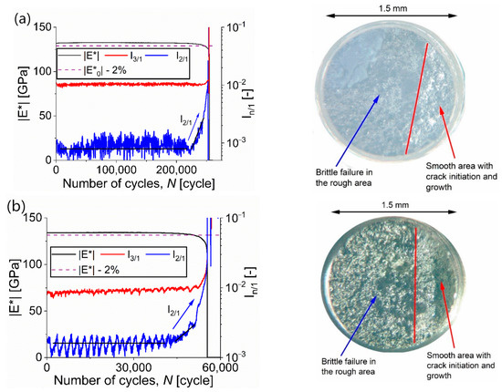
Figure 8.
Mechanical parameters (|E*|, I3/1 and I2/1) for a fatigue test of brass at ε0 = 0.1% (a) and ε0 = 0.14% (b) at 5 Hz, revealing the increase of the I2/1 intensity above the noise level after N = 220,000 and 45,000 cycles, respectively. On the right side the fracture surface is presented, using 40× magnification, revealing a smooth and a rough surface area, correlating with crack initiation and brittle failure, respectively.
The visual analysis of the fracture surface (fractography) shows for the six tests presented in Figure 6, Figure 7 and Figure 8 a smooth and a rough surface, which are separated by red lines as a guide for the eye. Cracks are generated and grow slowly in the smooth surface area [33], before fast crack growth occurs when the remaining cross-section area can no longer withstand the applied deformation. Therefore, it can be concluded that crack growth occurs, which can be followed in the mechanical stress response by the I2/1 intensity.
The decrease in the I2/1 intensity in Figure 6b, instead of the typical I2/1 increase with crack onset, can be explained by a vector compensation in a complex plane of the I2 contribution caused by the noise of the machine and the asymmetry in the force response caused by the crack initiation. When vectors of the noise of the machine and of the material response have a phase shift of 180°, they compensate each other resulting in an I2/1 decrease to a value close to zero (<10−4) followed by an intensity increase when the asymmetry of the material response, and consequently its vector in a complex plane, exceeds the noise level. Consequently, FT of the stress can detect cracks as soon as the I2/1 intensity significantly decreases or increases from the noise level.
7.2. The Rate of Change of I3/1 (dI3/1/dN) and the Cumulative Nonlinearity (Qf)
As seen in Figure 3, the I3/1 intensity quantifies the mechanical nonlinearity and increases linearly in regime II with ongoing fatigue with the cycle number as shown in Figure 4, so a constant slope can be determined. This slope (dI3/1/dN) was found to be correlated with the fatigue life time (Nf) for polymers [26]. The same analysis was performed for the metallic specimens and the results are presented in Figure 9a. It can be seen that a strong correlation exists between both parameters for all three materials.
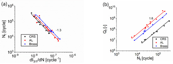
Figure 9.
(a) The number of cycles to failure (Nf) as a function of the rate of change of I3/1 (dI3/1/dN) in regime II for CRS (black square), AL (red circle) and brass (blue triangle), as well as their regression showing the same slope for all materials. (b) The correlation between the fatigue lifetime and the cumulative nonlinearity (Qf) also showing a high correlation with similar slope for the materials investigated.
The results of Figure 9a can be used to extract a power-law relation as:
with the proportionality factor AI3/1. Here, the exponents are the same (−1.3) for the three materials and the values of AI3/1 are reported in Table 1.

Table 1.
The proportionality factors (Astrain-life, AI3/1 and AQ) for the materials investigated, as well as their standard deviations as absolute and relative values for easier comparison. The lowest standard deviations are marked in bold.
The second nonlinear fatigue criterion investigated is the cumulative nonlinearity (Equations (10) and (11)) as reported in Figure 9b. A strong correlation between Nf and Qf is again observed as:
with a proportionality factor of AQ. Interestingly, the same exponent is obtained for all the materials investigated. CRS has the lowest Qf for a given fatigue lifetime compared with AL and brass, which also has shorter fatigue lifetimes under the same measurement conditions; i.e., shorter fatigue lifetime corresponds to a higher mechanical nonlinearity, which is quantified by AQ as reported in Table 1.
7.3. Comparison between the Nonlinear Parameters (dI3/1/dN and Qf) with the Strain-Life Curves—Standard Deviations Analysis
The prefactor Astrain-life, AI3/1 and AQ, as well as their standard deviations are listed and compared in Table 1. The lowest standard deviation (the best prediction) is marked in bold. While the standard deviation of the strain-life curve is in the range of 30–50%, the ones of the nonlinear criteria are only around 20%, revealing the lowest standard deviation for the two nonlinear criteria dI3/1/dN and Qf, with an even lower value for the Qf vs. Nf correlation. Similar results were observed for polymers in our recent studies [31].
7.4. Reproducibility under the Same Conditions
Using AL specimens, several tests were repeated under the same conditions (ε0 = 0.14%, ω1/2π = 5 Hz and R = 0.1) to investigate the reproducibility of the fatigue measurements. The strain-life (statistical) prediction is 31208 ± 8448 cycles, which represents a relative deviation of 27%. In contrast, the nonlinear predictions are more precise and predict Nf for each case individually better than the statistical prediction which gives in total a span of 22,760 cycles to 39,656 cycles, while the Nf via dI3/1/dN and Qf are typically within a 20% window of the measured fatigue lifetime. The results are compiled in Table 2 for simple analysis where the deviations are indicated.
Table 2.
The experimental results for four tests of AL at ε0 = 0.14%, ω1/2π = 5 Hz and R = 0.1, as well as the fatigue life predictions via the nonlinear parameters with their respective deviation in parenthesis.
8. Conclusions
The fatigue behavior of three metallic materials: cold rolled steel (CRS), aluminum (AL) and brass, was investigated via Fourier transform (FT) analysis of the force (stress) in displacement-controlled tests. Besides the fundamental harmonic at the frequency of the deformation input, higher harmonics at even and odd multiples of the fundamental harmonic were observed.
- For the undamaged specimen under large strain amplitudes, beyond the linear regime in a tensile test, the even higher harmonics were found to be within the noise of the machine, while the odd ones quantified the material nonlinearities.
- The intensity of the odd higher harmonics, in particular the first odd higher harmonic (I3/1), was found to scale quadratically with deformation (ε0), with intensities between 10−3 to 10−2.
- During a fatigue test, the I3/1 intensity was found to linearly increase with the cycle number (regime II) after a transient regime at the beginning of the test (regime I), before increasing rapidly at failure (regime III).
- Using the trend of the I3/1 intensity, the fatigue lifetime can be calculated from the constant I3/1 slope (dI3/1/dN) and the cumulative nonlinearity (Qf). The comparison between the power-law correlations for Nf (strain-life curves) revealed lower standard deviations, thus better fatigue predictions using I3/1.
- The I2/1 intensity is within the noise level at the beginning, but increased when crack initiation and propagation occurred as cracks create an asymmetry in the stress response due to a force reduction at the strain maximum and crack friction at the minimum.
- The I2/1 behavior was shown to be a powerful tool to detect and follow crack initiation and growth as it can quantify any asymmetry in the stress response, while I3/1 allowed to quantify the mechanical nonlinearity and its evolution due to fatigue, which can be used to predict failure.
Finally, the concept of FT analysis of the stress during fatigue testing was shown to be a powerful tool offering insights into the fatigue process from the time evolution of the mechanical stress response itself (before failure) and allowed better prediction (sensitivity and precision) than standard strain-life curves, while being able to detect cracks with high sensitivity.
For future work, the concepts developed here for other materials will be done, in particular for concrete due its wide use. Also, other testing conditions such as load controlled testing or random amplitude/frequency testing would be of high interest.
Author Contributions
Conceptualization, V.H. and D.R.; methodology, V.H.; software, V.H.; validation, V.H. and D.R.; formal analysis, V.H.; investigation, V.H.; resources, D.R.; data curation, V.H.; writing—original draft preparation, V.H.; writing—review and editing, D.R.; visualization, V.H.; supervision, D.R.; project administration, D.R.; funding acquisition, D.R. All authors have read and agreed to the published version of the manuscript.
Funding
This research was funded by the Natural Science and Engineering Research Council of Canada, grant number RGPIN-2016-05958.
Institutional Review Board Statement
Not applicable.
Informed Consent Statement
Not applicable.
Data Availability Statement
The data are available upon request.
Acknowledgments
The authors acknowledge the financial support of the Natural Sciences and Engineering Research Council of Canada (NSERC) and the technical support Yann Giroux.
Conflicts of Interest
The authors declare no conflict of interest.
References
- Bathias, C.; Pineau, A. Fatigue of Materials and Structures: Application to Design and Damage; John & Wiley & Sons: Hoboken, NJ, USA, 2013. [Google Scholar]
- Parvez, M.M.; Pan, T.; Chen, Y.; Karnati, S.; Newkirk, J.W.; Liou, F. High Cycle Fatigue Performance of LPBF 304L Stainless Steel at Nominal and Optimized Parameters. Materials 2020, 13, 1591. [Google Scholar] [CrossRef]
- Cui, W. A state-of-the-art review on fatigue life prediction methods for metal structures. J. Mar. Sci. Technol. 2002, 7, 43–56. [Google Scholar] [CrossRef]
- Liao, D.; Zhu, S.; Correia, J.A.; De Jesus, A.M.; Berto, F. Recent advances on notch effects in metal fatigue: A review. Fatigue Fract. Eng. Mater. Struct. 2020, 43, 637–659. [Google Scholar] [CrossRef]
- Qian, G.; Lei, W.-S. A statistical model of fatigue failure incorporating effects of specimen size and load amplitude on fatigue life. Philos. Mag. 2019, 99, 2089–2125. [Google Scholar] [CrossRef]
- Teng, Z.; Wu, H.; Boller, C.; Starke, P. A unified fatigue life calculation based on intrinsic thermal dissipation and microplasticity evolution. Int. J. Fatigue 2020, 131, 105370. [Google Scholar] [CrossRef]
- La Rosa, G.; Risitano, A. Thermographic methodology for rapid determination of the fatigue limit of materials and mechanical components. Int. J. Fatigue 2000, 22, 65–73. [Google Scholar] [CrossRef]
- Zhao, X.; Su, S.; Wang, W.; Zhang, X. Metal magnetic memory inspection of Q345B steel beam in four point bending fatigue test. J. Magn. Magn. Mater. 2020, 514, 167155. [Google Scholar] [CrossRef]
- Koch, A.; Wittke, P.; Walther, F. Computed Tomography-Based Characterization of the Fatigue Behavior and Damage Development of Extruded Profiles Made from Recycled AW6060 Aluminum Chips. Materials 2019, 12, 2372. [Google Scholar] [CrossRef] [PubMed]
- Zhu, B.; Lee, J. A Study on Fatigue State Evaluation of Rail by the Use of Ultrasonic Nonlinearity. Materials 2019, 12, 2698. [Google Scholar] [CrossRef]
- Santecchia, E.; Hamouda, A.M.S.; Musharavati, F.; Zalnezhad, E.; Cabibbo, M.; El Mehtedi, M.; Spigarelli, S. A Review on Fatigue Life Prediction Methods for Metals. Adv. Mater. Sci. Eng. 2016, 2016, 1–26. [Google Scholar] [CrossRef]
- Hyun, K.; Wilhelm, M.; Klein, C.O.; Cho, K.S.; Nam, J.G.; Ahn, K.H.; Lee, S.J.; Ewoldt, R.H.; McKinley, G.H. A review of nonlinear oscillatory shear tests: Analysis and application of large amplitude oscillatory shear (LAOS). Prog. Polym. Sci. 2011, 36, 1697–1753. [Google Scholar] [CrossRef]
- Wilhelm, M. Fourier-Transform Rheology. Macromol. Mater. Eng. 2002, 287, 83–105. [Google Scholar] [CrossRef]
- Bracewell, R. The Fourier Transform and Its Applications. Am. J. Phys. 1966, 34, 712. [Google Scholar] [CrossRef]
- Folland, G.B. Fourier Analysis and Its Applications; American Mathematical Society: Providence, RI, USA, 2009; Volume 4. [Google Scholar]
- Dessi, C.; Vlassopoulos, D.; Giacomin, A.J.; Saengow, C. Elastomers in oscillatory uniaxial extension. Rheol. Acta 2016, 56, 955–970. [Google Scholar] [CrossRef]
- Sagis, L.M.C.; Ramaekers, M.; Van Der Linden, E. Constitutive equations for an elastic material with anisotropic rigid particles. Phys. Rev. E 2001, 63, 051504. [Google Scholar] [CrossRef]
- Tsch, T.D.; Pollard, M.; Wilhelm, M. Kinetics of isothermal crystallization in isotactic polypropylene monitored with rheology and Fourier-transform rheology. J. Phys. Condens. Matter 2003, 15, S923–S931. [Google Scholar] [CrossRef]
- Hirschberg, V.; Wilhelm, M.; Rodrigue, D. Fatigue behavior of polystyrene (PS) analyzed from the Fourier transform (FT) of stress response: First evidence of I2/1(N) and I3/1(N) as new fingerprints. Polym. Test. 2017, 60, 343–350. [Google Scholar] [CrossRef]
- Cziep, M.A.; Abbasi, M.; Heck, M.; Arens, L.; Wilhelm, M. Effect of Molecular Weight, Polydispersity, and Monomer of Linear Homopolymer Melts on the Intrinsic Mechanical Nonlinearity 3Q0(ω) in MAOS. Macromolecules 2016, 49, 3566–3579. [Google Scholar] [CrossRef]
- Hirschberg, V.; Schwab, L.; Cziep, M.; Wilhelm, M.; Rodrigue, D. Influence of molecular properties on the mechanical fatigue of polystyrene (PS) analyzed via Wöhler curves and Fourier Transform rheology. Polymer 2018, 138, 1–7. [Google Scholar] [CrossRef]
- Hyun, K.; Wilhelm, M. Establishing a new mechanical nonlinear coefficient Q from FT-rheology: First investigation of entangled linear and comb polymer model systems. Macromolecules 2009, 42, 411–422. [Google Scholar] [CrossRef]
- Hirschberg, V.; Wilhelm, M.; Rodrigue, D. Fourier transform fatigue analysis of the stress in tension/tension of HDPE and PA6. Polym. Eng. Sci. 2020. [Google Scholar] [CrossRef]
- Campbell, F.C. Elements of Metallurgy and Engineering Alloys; ASM International: Novelty, OH, USA, 2008. [Google Scholar]
- Mortazavian, S.; Fatemi, A. Fatigue behavior and modeling of short fiber reinforced polymer composites: A literature review. Int. J. Fatigue 2015, 70, 297–321. [Google Scholar] [CrossRef]
- Hirschberg, V.; Wilhelm, M.; Rodrigue, D. Fatigue life prediction via the time-dependent evolution of linear and nonlinear mechanical parameters determined via Fourier transform of the stress. J. Appl. Polym. Sci. 2018, 135, 46634. [Google Scholar] [CrossRef]
- Hirschberg, V.; Wilhelm, M.; Rodrigue, D. Cumulative nonlinearity as a parameter to quantify mechanical fatigue. Fatigue Fract. Eng. Mater. Struct. 2019, 43, 265–276. [Google Scholar] [CrossRef]
- Ellyin, F. Fatigue Damage, Crack Growth and Life Prediction; Metzler, J.B., Ed.; Springer Science & Business Media: Berlin/Heidelberg, Germany, 1996. [Google Scholar]
- Halford, G. The energy required for fatigue (Plastic strain hysteresis energy required for fatigue in ferrous and nonferrous metals). J. Mater. 1966, 1, 3–18. [Google Scholar]
- van Dusschoten, D.; Wilhelm, M. Increased torque transducer sensitivity via oversampling. Rheol. Acta 2001, 40, 395–399. [Google Scholar] [CrossRef]
- Hirschberg, V.; Lacroix, F.; Wilhelm, M.; Rodrigue, D. Fatigue analysis of brittle polymers via Fourier transform of the stress. Mech. Mater. 2019, 137, 103100. [Google Scholar] [CrossRef]
- Hirschberg, V.; Wilhelm, M.; Rodrigue, D. Combining mechanical and thermal surface Fourier transform analysis to follow the dynamic fatigue behavior of polymers. Polym. Test. 2021, 96, 107070. [Google Scholar] [CrossRef]
- Song, Z.; Gao, W.; Wang, D.; Wu, Z.; Yan, M.; Huang, L.; Zhang, X. Very-High-Cycle Fatigue Behavior of Inconel 718 Alloy Fabricated by Selective Laser Melting at Elevated Temperature. Materials 2021, 14, 1001. [Google Scholar] [CrossRef]
Publisher’s Note: MDPI stays neutral with regard to jurisdictional claims in published maps and institutional affiliations. |
© 2021 by the authors. Licensee MDPI, Basel, Switzerland. This article is an open access article distributed under the terms and conditions of the Creative Commons Attribution (CC BY) license (https://creativecommons.org/licenses/by/4.0/).