Kriging Method-Based Return Prediction of Waste Electrical and Electronic Equipment in Reverse Logistics

Abstract

In reverse logistics, the accurate prediction of waste electrical and electronic equipment (WEEE) return amount is of great significance to guide electronic enterprises to formulate a reasonable recycling plan, remanufacturing production plan and inventory plan. However, due to the uncertainty of WEEE return, it is a challenge to accurately predict the WEEE return amount of recycling sites. Differently from the existing research methods aiming at the spatial correlation of the recycling amount of recycling sites, a spatial mathematical model based on Kriging method is proposed by this paper to predict the return amount of WEEE in reverse logistics. Based on the second-order randomness of the return amount, the spatial structure of the return amount of the recycling network is analyzed. According to the principle of unbiased prediction and minimum variance, the Kriging space mathematical model of WEEE return amount is derived, and the calculation process of three variograms is given. The results of Monte Carlo simulation and the case study on J company in Shanghai show that it is effective to utilize the Kriging method-based spatial mathematical model to predict the WEEE return of reverse logistics and analyze the spatial correlation structure of each recycling site. The proposed model can accurately predict the WEEE return amounts of unknown sites as well as those of the whole area through the known site data, which provides a novel analysis method and theoretical basis for the prediction of reverse logistics return amount.

1. Introduction

Humans are facing problems regarding the sustainability of the environment, such as increasing waste [1,2,3] and lack of resources [4,5,6]. The peak season of waste electrical and electronic equipment (WEEE) has come [7]. Not only is the amount of WEEE huge [8,9,10], the types of WEEE are continuously increasing and changing [11,12]. The closed-loop supply chain is critical [13,14,15]. The return and re-manufacturing of WEEE is key for recycling economy. In reverse logistics, it is very important to precisely predict the return of WEEE in order to make reasonable recycling plans [16,17], remanufacturing production plans [18,19,20], and inventory plans [21]. However, it is difficult for both academia and industry to predict WEEE return due to the uncertainty of the return amount.

Many achievements have been made by researchers in the field of return prediction for reverse logistics. These include prediction models based on the stochastic network: regarding the insufficient consideration of uncertainty and the randomness of recycling process in product recycling prediction research, Nelson et al. constructed a graphical evaluation and review technique (GERT) network prediction model for waste recycling treatment by using the random network method [22]. According to the time series data, the probability parameters and operation time participation of nodes in the GERT network are set and the product recycling amount is predicted through the network node transfer function.

There are also prediction models based on the regression equation: Kelle et al. studied the prediction of reverse logistics return volume [23]. They assumed that the product return volume was a function of product sales volume and return volume in the past, and built a return prediction model based on sales and recycling historical data. Colosimo et al. used a spatial autoregressive regression (SARX) model to characterize the roundness of a manufactured product [24]. Yang and Williams established a logistic regression model to predict the trend of waste computers [25]. The polynomial regression analysis is good at fitting the trend of polynomials in a data series but the highest idempotent of polynomials mainly depends on human choice, especially the power of polynomial items is assumed to be integers, which will lead to model errors.

In terms of prediction models based on neural network, based on the back propagation (BP) neural network prediction method, Li and Tee constructed a combined forecasting model of return neural network to predict the product return [26]. Gómez et al. proposed a reverse logistics forecasting model based on the neural network method after analyzing the disadvantages of common prediction methods such as moving average method, exponential smoothing method and causal analysis method [27]. The modeling process is mainly reflected in two aspects: one is the representation structure of the prediction network, and the other one is the number of nodes in the input/output layer, hidden layer and output layer of the network. The input layer is the factor affecting the return amount, the intermediate layer is the neuron set by the user according to the actual problem, and the output layer is the return amount on the time series to be predicted.

Neural network is a modeling tool which has developed rapidly in the past 20 years [28,29,30]. It can be used for regression modeling and autoregressive modeling when it is used to predict the return amount based on time series. However, the main problem with this method is that the network structure and the number of nodes need to be determined by users’ experience, and there is no clear mathematical analysis guidance. For example, the number of nodes in the input layer and output layer requires users’ experience. If the number of nodes is too small, it will affect the effectiveness of the prediction, and too many nodes will affect the training time and efficiency. In addition, there are some problems such as over fitting, especially the poor generalization ability of extrapolation.

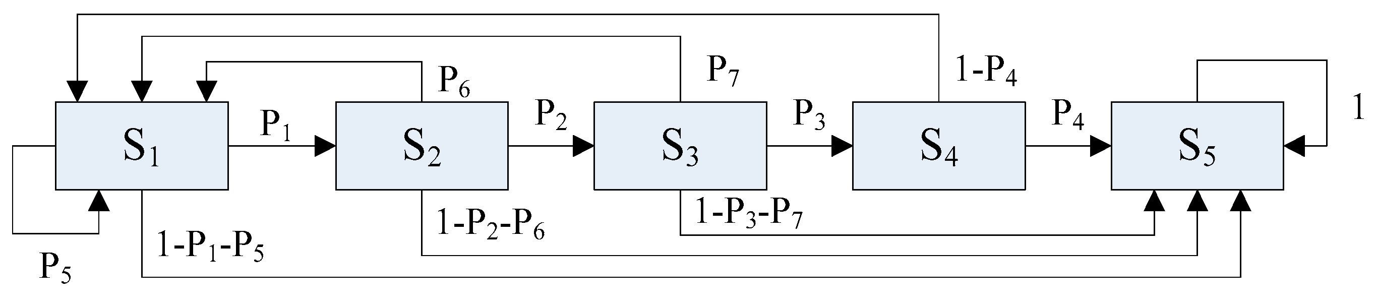
Based on the Markov prediction model: Lakshmanan et al. established the Markov model to predict the quantity of recovered products in different states at the end of a certain period [31]. The Markov chain organically combines the prediction of product state quantity and time, which proves the validity of the Markov model in theory. Peng and Dong (2011) established a Markov prediction model considering the two states of recycled products after treatment [32]. The prediction model of reverse logistics return based on the Markov process can be expressed in Figure 1, where $S$ is the different state of the product, and $P$ is the probability.

The Markov process in Figure 1 is described by the probability matrix of product state transition, and the return amount of waste products is predicted. The Markov method makes full use of the correlation between product states, and the example results show that the Markov method has advantages in predicting the return amount based on the correlation of time series.

Prediction model based on Grey Theory: Wu et al. established grey theory prediction of plastic product return of enterprises [33]. The grey model method is a dynamic model of difference equation of discrete time series. Wang and Hsu proposed an improved grey transfer function noise two-stage prediction model [34]. Prediction model based on fuzzy intelligence: Bhola et al. put forward a method to establish the prediction model of recycling quantity by using a fuzzy model reasoning system based on analyzing the main factors affecting the reverse logistics [35]. The fuzzy intelligence model uses fuzzy theory to express fuzzy information and fuzzy knowledge in digital way, which realizes the organic combination of symbolic intelligence and computational intelligence. The Mamdani fuzzy inference system is used to predict the recycling of waste machine tools, and good prediction results are obtained. However, the model makes important assumptions about business return and incentive mechanism, which needs to be modified according to the actual situation, otherwise it has certain limitations.

Prediction model based on Bayes method: Rivoirard assumes that in the reverse logistics volume of products follows binomial probability distribution, and Bayesian inference and expectation maximization algorithm are used to solve the total probability and backward logistics lag probability parameters of a product, so as to determine the quantity and time of product return [36].

In the above study, the amount of waste products recovered from each recycling site in the reverse logistics network is predicted as the time series data, mainly considering the time correlation of the data. These methods have achieved good prediction results under certain applicable conditions. However, in WEEE reverse logistics, the return amount of each recycling network is not only related in the time sequence, but also has spatial correlation between different recycling sites.

Assuming that an electronic company owns$q$ recycling sites in a limited two-dimensional area $\mathit{D}$ (see Figure 2), the recycling sites can be denoted by $s_i\left(x,y\right)$ ($i=1,2,\dots ,q$), where $x$ and $y$ represent the abscissa and ordinate of the geographical location of the recycling site in $\mathit{D}$ respectively. The distance between any two recycling sites is denoted by $h$. The recycling sites denoted by $s_i\left(x,y\right)$ ($i=1,2,\dots ,q$) can be rewritten in vector form as $\mathit{S}\left(s_1,s_2,\cdots ,s_q\right)$. The return amount of each site, denoted by $\left(s_i\right)$ $\left(i=1,2,\dots ,q\right)$, can be rewritten in vector form as $\mathit{Z}\left(Z\left(s_1\right),\hspace{0.17em}Z\left(s_2\right),\hspace{0.17em}\cdots ,Z\left(s_q\right)\right)$ and considered as a random variable.

Considering random disturbance, in a certain period, the return amounts of arbitrary $n (n<q)$ recycling sites can be obtained by detection and denoted by $Z\left(s_1\right),\hspace{0.17em}Z\left(s_2\right),\hspace{0.17em}\cdots ,Z\left(s_n\right)$ respectively. There are two challenges for researchers to deal with.

Challenge 1: It is difficult to obtain a quantitative description for the spatial structure correlation between the given $Z\left(s_i\right) \left(i=1,2,\dots ,n\right)$ and the unknown $\widehat{Z}\left(s_i\right), \left(i=n+1,n+2,\dots ,q\right)$.

Challenge 2: Even though the quantitative description of the spatial structure correlation is obtained, it is hard to predict the unknown $\widehat{Z}\left(s_i\right) \left(i=n+1,n+2,\dots ,q\right)$ based on the given return amounts of $n$ recycling sites, which will result in an accurate prediction of the return amounts of all the recycling sites in area $\mathit{D}$.

In order to solve the above two challenges, it is necessary to analyze the spatial structure of the return amounts between recycling sites under the conditions of spatial correlation and randomness and establish a spatial correlation random model.

Firstly, correlation arises frequently in data observed within certain intervals of space, and the data indeed exhibit a significant amount of positive autocorrelation. The waste electrical and electronic equipment (WEEE) return amounts in every recycling sites are often spatially correlated because they are obtained in similar conditions during the recycling process and related to similar properties. Spatial correlation is different from temporal correlation, which is usually represented via time series models. In fact, spatial correlation models allow one to represent contiguity in space rather than in time.

Therefore, it is vital for us to develop a quantitative mathematical description model of the spatial structure correlation between the given return amounts and the unknown return amounts. In the practical application of the space modeling method for spatial correlation, an important assumption is the second-order randomness, which means that the variables can be arbitrary values in a certain period. The second-order randomness means that the properties of the random function satisfied by the variables remain unchanged. The mean value of the random function is a constant. And the covariance between the random recoveries of any two nodes, only depends on the distance between them. The first scientific issue we need to handle is to prove that the spatial structure of the return amount of the recycling network follows the second-order randomness property. If the property is proved to be true, the quantitative mathematical description model of the spatial structure correlation could be developed.

Secondly, the second scientific issue is to develop a mathematical prediction model to predict the unknown return amounts based on the given return amounts of n recycling sites. It is difficult for both academia and industry to predict the WEEE return due to the uncertainty of the return amount. The return estimation amounts are not exactly equal to the real amounts. There is a deviation between the estimation and the real amount, which leads to the inaccuracy prediction. The reason for this phenomenon is that predicting the return values only uses known value information on measured recycling sites considering the spatial correlation. Therefore, developing a mathematical prediction model and decrease this deviation to improve the precision of WEEE return amount prediction is another crucial scientific issue.

The kriging method is one of most important meta-modeling methods to predict the responses at unknown points from some observed data [37], and the prediction is based on the spatial structure correlation, which makes it quite suitable for challenge 2. In addition, the closed-form formula of the predictor can be derived, which makes the method easy to implement. The kriging method can also be extended to consider random noise at the same point, such as stochastic kriging [38], which meets the demand of the studied problem.

One of the main factors that affect the performance of the kriging predictor is the choices of the correlation function, which is usually application-dependent. Thus, several spatial structure correlation functions, i.e., the variogram functions, are developed based on the features of the problem and compared to solve challenge 1. This is one of the main contribution in this paper.

The kriging method is one of the most important meta-models for the spatial structure correlation analysis in a random field [39,40]. Detailed descriptions of existing research on Kriging meta-modeling are provided in review [41].

Little research on WEEE return prediction considering spatial correlation has been conducted, and the literature on this topic is sparse. In contrast to the current methods, in this paper, a new mathematical spatial model for predicting WEEE return in reverse logistics based on Kriging method [42] is developed, considering the spatial correlation of the WEEE return amounts of different recycling sites. The spatial statistics based on Kriging method has been widely applied in many scientific fields such as geography, agrology, and meteorology. This study analyzes the spatial variogram structure considering the spatial correlation based on the Kriging method.

Firstly, the WEEE recycling system is described. The second order randomness and the spatial structure of the WEEE return are analyzed. Secondly, the Kriging spatial model of WEEE return prediction is explored, and three variograms including spherical, exponential, and Gaussian variogram for prediction of WEEE return are calculated by the Monte Carlo simulation. Thirdly, a case study based on actual data is presented. The developed spatial prediction model can be used as a novel method and theory analysis tool for the prediction of WEEE return in reverse logistics.

The rest of this paper is organized as follows. The spatial model based on Kriging method for WEEE return prediction is developed in Section 2, which considers both the randomness of the return amount and the spatial correlation between two different recycling sites. In Section 3, the simulation experiment and performance analysis are conducted based on the Monte Carlo method. In Section 4, a case study is presented to validate the proposed model based on the actual data. Finally, conclusions are given in Section 5.

2. The Proposed Approach

The main contribution of this paper is to develop a spatial mathematical model based on Kriging method to predict the return amount of WEEE in reverse logistics. To obtain the prediction model, the fact that the spatial structure of the return amount of the recycling network follows the second-order randomness property is firstly demonstrated, and the variogram functions to describe the spatial variation structure among the random variables of return amount are explored.

2.1. Second-Order Randomness Hypothesis of the Kriging Method

In the practical application of the Kriging space modeling method, an important assumption is second-order randomness [38], which means that the variables can be arbitrary values in a certain period. Second-order randomness means that the properties of the random function satisfied by the variables remain unchanged. The mean value of the random function is a constant. Moreover, the covariance between the random recoveries of any two nodes, denoted by $\mathrm{cov}\left[s_i\left(x,y\right),s_j\left(x,y\right)\right]$, only depends on the distance between them, where $x$ and $y$ represent the abscissa and ordinate of the geographical location of the recycling site.

Denoting the total amount of return within the area $\mathit{D}$ in a certain period by $m$, the second order randomness can be expressed as

$$E\left[Z\left(s\right)\right]=m,\left(s\in \mathit{D}\right)$$

(1)

$$Cov\left[Z\left(s+h\right),Z\left(s\right)\right]=C\left(h\right),\left(s,s+h\in \mathit{D}\right)$$

(2)

where $s$ presents a certain recycling site in the area $D$ and $\left(s+h\right)$ presents a recycling site that has distance $h$ from the site $s$. E, $Cov$ and $Z\left(s+h\right)$ represent the expected value of a random variable, the covariance of two random variables, and the return amount of the recycling site which is h away from the site s respectively.

2.2. Demonstration of Hypothesis Rationality

In this paper, it is assumed that the return of WEEE reverse logistics sites conforms to the second-order randomness, and the demonstration is given as follows.

(1) From the perspective of the research object: the Kriging method traditionally studies the storage capacity of ore in different mines in a certain area, and different mines are represented by geographical coordinates. The research object of this paper is the WEEE return amount of different recycling sites in a certain area, and each recycling site is also represented by geographical coordinates. Both studies are aimed at the spatial relationship between variables with a correlation under different geographical coordinates in a certain area, and the situation is similar.

(2) From the perspective of randomness: traditionally, the Kriging method predicts the ore quantity of unknown mines by the ore quantity of several known mines, and the ore quantity of each mine is uncertain and random. In this paper, the Kriging method is used to predict the WEEE return amounts of the unknown recycling site based on the return amounts of several known sites. The return amount of each site is also uncertain and random.

(3) From the perspective of the constant overall mean value: due to the formation of geological structure, the total amount of ore storage in a certain area is determined, and the overall mean value is unchanged. Nevertheless, the distribution of ore storage amounts among different mines are different. For WEEE recycling, as long as the environmental protection related laws, regulations, policies and the environmental awareness of the residents remain stable in a certain area, the overall return amount of WEEE will not change much. Meanwhile, the return amounts of different recycling sites will be distributed randomly and differently, which is the same as the ore storage distribution.

(4) From the perspective of the covariance analysis: whether it is in case of ore volume prediction or WEEE return prediction, the covariance of ore storage/return amount of any two mines/recycling sites is only dependent on the distance between these two mines/recycling sites. The farther the distance is, the weaker the correlation will be, and vice versa. From this perspective, the properties of covariance in these two cases are similar.

The results of category demonstration are shown by

Table 1. Demonstration of WEEE return in accordance with the second-order randomness hypothesis.

Scenarios		Ore Quantity Prediction	WEEE Return Amount Prediction
Objective		The storage capacity of ore in different mines in a certain area.	Return amount of WEEE in each recycling site in a certain area.
Randomness		The storage capacity of a certain ore in different mines is uncertain and random.	The return amount of WEEE in each recycling site is uncertain and random.
Second order randomness	Mean value is constant.	The total amount of ore is stable.	The return amount is stable in a certain period.
	Covariance only depends on the variable distance.	There is a correlation among the ore quantity in different mines, which is weaker as the distance gets greater.	The WEEE return amounts of different sites are correlated, which is weaker as the distance gets greater.

.

Therefore, compared with the traditional ore storage, the WEEE return in this paper conforms to the second-order randomness hypothesis of Kriging method.

2.3. Spatial Structure Analysis of WEEE Recycling Sites

In this paper, the variogram, first proposed in spatial statistics, is used to describe the spatial variation structure among the random variables of return amount. Denoting the variogram by γ($h$), the limited variance of [Z(s + $h$) − Z(s)] can be formulated as

$$\begin{array}{l}Var\left[Z\left(s+h\right)-Z\left(s\right)\right]=E\{\left\{\left[Z\left(s+h\right)-Z\left(s\right)\right]-E\left[Z\left(s+h\right)-Z\left(s\right)\right]{\}}^2\right\}\\ =E\left\{{[Z\left(s+h\right)-Z\left(s\right)]}^2\right\}=2\gamma \left(h\right)\end{array}$$

(3)

Under the assumption of second-order randomness, the properties of the spatial structure of recycling sites in WEEE reverse logistics are summarized as follows.

Property 1: In the whole area $\mathit{D}$, the mathematical relationship between the spatial variogram and return amounts of different recycling sites is given by

$$\gamma \left(h\right)={\sigma }^2-C\left(h\right)$$

(4)

where ${\sigma }^2$ and $C\left(h\right)$ denote the variance and covariance, formulated by Equations (5) and (6) respectively.

$${\sigma }^2=Var\left[Z\left(s\right)\right]=E\left\{{[Z\left(s\right)-m]}^2\right\}$$

(5)

$$C\left(h\right)=Cov\left[Z\left(s+h\right),Z\left(s\right)\right]=E\left[Z\left(s+h\right)-m\right]\left[Z\left(s\right)-m\right]=E\left[Z\left(s+h\right)Z\left(s\right)\right]-m^2$$

(6)

The proof of Property 1 is given as follows.

$$\begin{array}{ll}2\gamma \left(h\right)& =E\left\{{[Z\left(s\right)-m]}^2\right\}=E\{\left\{\left[Z\left(s+h\right)-m\right]-\left[Z\left(s\right)-m\right]{\}}^2\right\}\\ & =E\left\{\left[Z\left(s+h\right)-m{]}^2-2\left[Z\left(s\right)-m\right]\left[Z\left(s+h\right)-m\right]+\right[Z\left(s\right)-m{]}^2\right\}\\ & =E\left\{{[Z\left(s+h\right)-m]}^2\right\}-2E\left\{\left[Z\left(s\right)-m\right]\left[Z\left(s+h\right)-m\right]\right\}+E\left\{{[Z\left(s\right)-m]}^2\right\}\\ & ={\sigma }^2-2C\left(h\right)+{\sigma }^2=2{\sigma }^2-2C\left(h\right)\end{array}$$

(7)

Property 2: In the whole area $\mathit{D}$, the mathematical relationship between the spatial variogram and return amount of a single recycling site is given by

$$\gamma \left(h\right)={\sigma }^2\left[1-\rho \left(h\right)\right]$$

(8)

where $\rho \left(h\right)$ is the spatial correlation coefficient, defined by $\rho \left(h\right)=0.5C\left(h\right)/{\sigma }^2$.

The proof of Property 2 is given as follows.

According to Equation (3) and the definition of $\rho \left(h\right)$, it can be derived that

$$\begin{array}{ll}\gamma \left(h\right)& ={\sigma }^2-C\left(h\right)={\sigma }^2\left[1-0.5C\left(h\right)/{\sigma }^2\right]\\ & ={\sigma }^2\left[1-\rho \left(h\right)\right]\end{array}$$

(9)

2.4. Variogram of WEEE Return Amount

The return variogram reveals the spatial variation degree and correlation structure of the WEEE return amount in different spatial locations of the recycling network in the whole area D, indicating the randomness as well as the structure characteristics at the same time. Taking the variogram value as the Y-axis and the distance between two different recycling sites h as the x-axis, the spatial variogram of WEEE return amount in recycling sites is shown as Figure 3.

There are several concepts that need to be illustrated in Figure 3. Firstly, when the distance $h=0$, the variogram value $\gamma \left(0\right)$ is termed as the nugget and denoted by $C_0$, reflecting the variation caused by sampling scale and other factors. Secondly, the return variogram $\gamma \left(h\right)$ continuously increases from non-zero value and finally reaches a relatively stable constant as the distance between two different recycling sites $h$ grows. Moreover, this constant value is termed as sill and denoted by $C_0+C_1$, indicating the maximum variation range or total variation degree of the WEEE return amount of each recycling site. Thirdly, when the return variogram value reaches sill, the distance is termed as the correlation length and denoted by $a$, which means $\gamma \left(a\right)=C_0+C_1$. If and only if the distance between two recycling sites is less than the correlation length, i.e., $h<a$, the detected values is deemed as spatially correlated. Otherwise, the spatial correlation is too weak to worth consideration and thus can be negligible in this study.

In spatial statistics, the commonly used spatial variograms include spherical, exponential, and Gaussian variogram, which have been proved to be effective for analysis of spatial variation structure. Three kinds of return variogram employed in this paper are given as follows.

(1) The spherical variogram is formulated as

$$\gamma \left(h\right)=\{\begin{array}{c}{C}_0+C_1[1.5\left(h/a\right)-0.5\left(h/a{)}^3\right],0\le h\le a\\ C_0+C_1,h>\mathrm{a}\end{array}$$

(10)

The corresponding covariance function is given by

$$C\left(h\right)=\{\begin{array}{c}{C}_0+C_1,h=0\\ C_1[1-1.5\left(h/a\right)+0.5\left(h/a{)}^3\right],0<h\le a\\ 0,h>a\end{array}$$

(11)

(2) The exponential variogram is formulated as

$$\gamma \left(h\right)=C_0+C_1\left(1-e^{-3h/a}\right)$$

(12)

And its corresponding covariance function is given by

$$C\left(h\right)=C_0+C_1{e}^{-3h/a}$$

(13)

(3) The Gaussian variogram is formulated as

$$\gamma \left(h\right)=C_0+C_1\left(1-e^{-3{(h/a)}^2}\right)$$

(14)

The corresponding covariance function is given by

$$C\left(h\right)=C_0+C_1{e}^{-3{(h/a)}^2}$$

(15)

Note that the degree of spatial variability can be expressed by dividing the variation range between nodes $C_1$ by the total variation degree of the system $C_0+C_1$, that is, the structural variance ratio $\frac{C_1}{C_0+C_1}$. This ratio indicates the proportion of the spatial variation caused by the autocorrelation part of the return amount in the total variation of the system, and can reflect the spatial correlation degree of the return variable. In reverse logistics, if the structural variance ratio is less than 25%, it means that there is a weak spatial correlation between the return variables of different recycling sites; when this ratio is within the range of 25–75%, the return variables have a moderate spatial correlation; when this ratio is more than 75%, the spatial correlation between return variables is deemed to be strong.

2.5. Kriging Spatial Model for Prediction of WEEE Return

The Kriging method is the most important spatial prediction method of random variables in spatial statistics. According to the review, this method has not been applied to the prediction of the WEEE return in reverse logistics network. In this paper, based on the second-order randomness and the spatial properties of the return amount in the recycling network, the WEEE return Kriging spatial prediction model is derived.

The prediction value of WEEE return amount of an arbitrary recycling site $\widehat{Z}\left(s_0\right)$ can be transformed into the linear combination of the known return amounts of $n$ recycling sites, given as

$$\widehat{Z}\left(s_0\right)=m+{\displaystyle \sum }_{i=1}^n{\lambda }_i\left[Z\left(s_i\right)-m\right]$$

(16)

where $Z\left(s_i\right)$ refers to the known return amount of recycling site $s_i$, and ${\lambda }_i$ is the corresponding weight.

The key to accurately predict the unknown network return is to calculate the reasonable weight ${\lambda }_i$. It is important for WEEE return prediction to satisfy the unbiased prediction condition and to minimize the prediction variance. The calculation of ${\lambda }_i$ is discussed from these two aspects.

In order to construct the unbiased prediction, the average prediction error should be 0, which can be expressed by

$$E\left[\widehat{Z}\left(s_0\right)-Z\left(s_0\right)\right]=0$$

(17)

Substituting Equation (15) into Equation (16), yields

$$E\left[\widehat{Z}\left(s_0\right)-Z\left(s_0\right)\right]=m+{\displaystyle \sum }_{i=1}^n{\lambda }_i\left\{m-m\right\}-m=0$$

(18)

Equation (18) can be further derived as

$$E\left[\widehat{Z}\left(s_0\right)-Z\left(s_0\right)\right]=m+{\displaystyle \sum }_{i=1}^n{\lambda }_i\left\{m-m\right\}-m=0$$

(19)

According to Equation (18), no matter how the weight ${\lambda }_i$ is set, the prediction of return amount is unbiased, which means that the return prediction based on Kriging method is effective.

The prediction variance minimization, the variance between the predicted value and the true value can be expressed as

$$Var\left[\widehat{Z}\left(s_0\right)-Z\left(s_0\right)\right]={\sigma }^2-2{\displaystyle \sum }_{i=1}^n{\lambda }_{i}C\left(s_0-s_i\right)+{\displaystyle \sum }_{i=1}^n{\displaystyle \sum }_{j=1}^n{\lambda }_i{\lambda }_{j}C\left(s_i-s_j\right)=\Sigma$$

(20)

where ${\sigma }^2$ denotes the variance of the randomness $Z\left({\mathrm{s}}_0\right)$ defined in Equation (5), and $\Sigma$ denotes the variance between the predicted value and the true value. To minimize $\Sigma$, the weight ${\lambda }_i$ could be calculated by

$$\left[\begin{array}{c}{\lambda }_1\\ ⋮\\ {\lambda }_n\end{array}\right]={\left[\begin{array}{ccc}{C}_{11}& \cdots & C_{1n}\\ ⋮& \ddots & ⋮\\ C_{n1}& \cdots & C_{nn}\end{array}\right]}^{-1}\left[\begin{array}{c}{C}_{01}\\ ⋮\\ C_{0n}\end{array}\right]$$

(21)

where $C_{ij}$ is the covariance of $s_i$ and $s_j$, given by $C_{ij}=Cov(s_i-s_j)$.

The proof of Equation (20) is shown as follows. If the prediction variance of the Kriging method is minimized, the Kriging linear calculation equation of weight ${\lambda }_i$ can be formulated as

$$\begin{array}{l}\Sigma ={\sigma }^2-2{\lambda }_{1}C(s_0-s_1)+{\lambda }_{2}C(s_0-s_2)+\dots +{\lambda }_{n}C(s_0-s_n)]\\ \begin{array}{cc}& \end{array}+{\lambda }_1[{\lambda }_{1}C(s_1-s_1)+{\lambda }_{2}C(s_1-s_2)+\dots +{\lambda }_{n}C(s_1-s_n)]\\ \begin{array}{cc}& \end{array}+{\lambda }_2[{\lambda }_{1}C(s_2-s_1)+{\lambda }_{2}C(s_2-s_2)+\dots +{\lambda }_{n}C(s_2-s_n)]\\ \begin{array}{cc}& \end{array}+\cdots \\ \begin{array}{cc}& \end{array}+{\lambda }_n[{\lambda }_{1}C(s_n-s_1)+{\lambda }_{2}C(s_n-s_2)+\dots +{\lambda }_{n}C(s_n-s_n)]\end{array}$$

(22)

where ${\sigma }^2$ denotes the variance of the randomness $Z\left({\mathrm{s}}_0\right)$ defined in Equation (5).

In case of $i=1$, taking the first partial derivative of the right side of Equation (21), and setting it to 0, yields

$$\begin{array}{l}\frac{\partial S}{\partial {\lambda }_1}=-2C(s_0-s_1)+[2{\lambda }_{1}C(s_1-s_1)+{\lambda }_{2}C(s_1-s_2)+\dots +{\lambda }_{n}C(s_1-s_n)]+{\lambda }_{2}C(s_2-s_1)+\dots +{\lambda }_{n}C(s_n-s_1)\\ \begin{array}{cc}& \end{array}=-2C(s_0-s_1)+2[{\lambda }_{1}C(s_1-s_1)+{\lambda }_{2}C(s_1-s_2)+\dots +{\lambda }_{n}C(s_1-s_n)]\\ \begin{array}{cc}& \end{array}=0\end{array}$$

(23)

And Equation (23) can be further derived as

$${\lambda }_{1}C(s_1-s_1)+{\lambda }_{2}C(s_1-s_2)+\dots +{\lambda }_{n}C(s_1-s_n)=C(s_0-s_1)$$

(24)

Moreover, Equation (23) can be simplified as

$${\lambda }_1{C}_{11}+{\lambda }_2{C}_{12}+\cdots +{\lambda }_n{C}_{1n}=C_{01}$$

(25)

According to the mathematical induction, for each weight ${\lambda }_i \left(i=1,2,\dots ,n\right)$ in Equation (21), it can be obtained that

$${\lambda }_1{C}_{n1}+{\lambda }_2{C}_{n2}+\cdots +{\lambda }_n{C}_{nn}=C_{0n}$$

(26)

The linear equations are expressed by

$${\displaystyle \sum _{i=1}^n{\lambda }_{i}C(s_i-s_j)}=C(s_0-s_j),j=1,\dots ,n$$

(27)

Converting Equation (27) into matrix form yields

$$\left[\begin{array}{ccc}{C}_{11}& \cdots & C_{1n}\\ ⋮& \ddots & ⋮\\ C_{n1}& \cdots & C_{nn}\end{array}\right]\left[\begin{array}{c}{\lambda }_1\\ ⋮\\ {\lambda }_n\end{array}\right]=\left[\begin{array}{c}{C}_{01}\\ ⋮\\ C_{0n}\end{array}\right]$$

(28)

By substituting Equation (20) into Equation (15), the unbiased prediction value of WEEE return with minimum variance $\widehat{Z}\left(s_0\right)$ can be obtained. The variance between predicted and true values is formulated as

$${\sigma }_{SK}{}^2=Var[\widehat{Z}(s_0)-Z(s_0)]={\sigma }^2-{\displaystyle \sum _{i=1}^n{\lambda }_{i}C(s_0-s_i)}$$

(29)

Therefore, the WEEE return of an arbitrary recycling site in the whole area $\mathit{D}$ can be predicted through Equations (15)–(20).

3. Monte Carlo simulation

3.1. Monte Carlo Simulation Data Generation

The Monte Carlo method is an important method for stochastic process simulation, which is widely used in various scientific simulation calculations. In this paper, the Monte Carlo random variable simulation method is used to generate a large amount of data with a spatial correlation structure for simulation experiments. The simulation data is generated in MATLAB software environment. The simulation purposes are as follows: (1) to verify the correctness of the proposed spatial model of WEEE return; (2) to analyze which variogram is more suitable for the variation structure analysis of WEEE return network.

Considering a company recycles printers in Shanghai, the Monte Carlo method is utilized to randomly generate four samples with spatial correlation (as shown in

Table 2. Sample data of Monte Carlo simulation.

No. of Samples	No. of Sites	Repetitions	Min.	Max.	Median	Standard Deviation
1	100	25	0	9543	5421	0.0026
2	50	50	0	8945	4580	0.0027
3	20	50	0	10000	5110	0.0025
4	10	50	0	7849	3459	0.0026

).

The numbers of recycling sites in Shanghai for each sample are 100, 50, 20 and 10 respectively, which can basically cover the actual range of possible number of recycling sites. For samples 2, 3 and 4, the simulation is repeated for 50 times. For sample 1, because there are 100 sites, the computation load is too large. Thus, the simulation for sample 1 is repeated 25 times. The number of repetitions is set to achieve a good standard deviation, as shown in Table 2. The detailed statistical description is given in Table 2. For samples 1, 2, 3 and 4, the return amounts of 80, 40, 16 and eight sites are known respectively. The remaining 20% return of each sample is used as the test. The prediction value calculated by the proposed method is compared with these test samples to verify the correctness of the method.

3.2. Spatial Structure Analysis and Variogram Calculation Results

The variogram functions provide an effective solution for the spatial correlation data analysis of printer return. Three commonly used variograms, namely spherical, exponential, and Gaussian variogram, can be used in the Kriging spatial model for return prediction. As shown in Figure 4, three variogram functions are finally fitted after repeated simulation.

Note that the abscissa unit in Figure 4 is 0.5 km, which does not mean that the interval between two recycling sites must be set to 0.5 km in practice. In order to find out the variation law as well as the spatial structure of return amount, the sampling points should be set as densely as possible, within the limit of computing capability. It can be seen from Figure 4 that the variation structure analysis covers the range from 0.5 km to 100 km. The corresponding variation value can be found as long as the distance between recycling sites is within this range (for example, two recycling sites with a distance of 20 km).

Simulation conclusion 1: As can be seen from Figure 4, the correlation length of these three variogram functions is about 90 km, that is, if the distance between two recycling sites exceeds 90 km, the correlation will decrease quickly.

Figure 4 shows the results of quantitative comparative analysis of structural variance of different site numbers. The larger the structural variance ratio $\frac{C_1}{C_0+C_1}$, the stronger the spatial correlation will be.

Simulation conclusion 2: The prediction value given by the Kriging method using exponential variogram is the best and its prediction error is the least. It can be found from

Table 3. Quantitative analysis results of three different variograms.

No. of Sites	Variogram	$\mathbf{Sill}({\mathit{C}}_0+{\mathit{C}}_1)$	$\mathbf{Nugget}\left({\mathit{C}}_0\right)$	Structural Variance Ratio
100	Spherical	0.80778	0.14828	81.64%
	Exponential	0.80664	0.10263	87.28%
	Gaussian	0.81273	0.24242	70.17%
50	Spherical	0.82451	0.14717	82.15%
	Exponential	0.84158	0.08912	89.41%
	Gaussian	0.82170	0.18225	77.82%
20	Spherical	0.90012	0.14104	84.33%
	Exponential	0.92157	0.09086	90.14%
	Gaussian	0.92108	0.16422	82.17%
10	Spherical	0.94212	0.11194	88.12%
	Exponential	0.94852	0.55578	94.15%
	Gaussian	0.92349	0.21733	76.47%

that the structural variance ratio fitted by exponential variogram is the largest, indicating the WEEE return of each recycling site has the strongest spatial correlation, which is most consistent with the Monte Carlo simulation test data.

3.3. Prediction Results of WEEE Return Kriging Model

The prediction accuracy of the Kriging method is evaluated by prediction error percentage (PEP) and standard deviation of prediction error (SDPE). The prediction error percentage is the difference between the real value and the predicted value divided by the real value, and the standard deviation of prediction error is the standard deviation of Kriging prediction error of multiple samples. The prediction results of the WEEE return Kriging spatial model proposed in this paper are shown in

Table 4. Evaluation of prediction results of WEEE Kriging model for simulation.

No. of Sites	Variogram	PEP	SDPE
100	Spherical	1.08%	0.015657
	Exponential	0.87%	0.016062
	Gaussian	1.71%	0.012183
50	Spherical	1.04%	0.014249
	Exponential	0.84%	0.012343
	Gaussian	1.76%	0.014894
20	Spherical	0.84%	0.014158
	Exponential	0.48%	0.018421
	Gaussian	1.42%	0.019510
10	Spherical	1.07%	0.016518
	Exponential	0.87%	0.014328
	Gaussian	2.49%	0.015571
Total		1.21%	0.001532

.

Simulation conclusion 3: The total prediction error percentage is 1.21%, and the standard deviation is 0.001532 which demonstrates that the proposed model can accurately predict the return of WEEE in reverse logistics. Moreover, the correctness of the method is also verified. The calculation result here refers to the average value of each sample repeated several times in all recycling sites in the whole area.

Simulation conclusion 4: From the perspective of variogram, the prediction error percentage of exponential variogram is 0.77%, which is lower than that of spherical variogram (1.01%) and Gaussian variogram (1.85%). The main reason for the low accuracy of Gaussian variogram is that the slope of Gaussian variogram at the origin is 0, which leads to the instability and abnormal phenomenon of Kriging prediction.

Simulation conclusion 5: According to the influence of the number of recycling sites on the performance of the prediction model, the prediction error percentages of 100, 50, 20 and 10 are 1.22%, 1.21%, 0.91% and 1.48%, respectively. There is no significant fluctuation of prediction error. This also shows that the return Kriging model is applicable to a WEEE reverse logistics return system with different number of recycling sites, and the proposed model is universal.

4. Case Study

In order to further verify the correctness of the spatial mathematical model of WEEE return prediction of reverse logistics based on the Kriging method, the WEEE return prediction of J company is taken as an example for case study in this paper. J company is one of the key national eco city demonstration enterprises in Shanghai, China. With the goal of promoting the rational utilization of resources, J company is committed to becoming a comprehensive service provider of renewable resources industrial chain. Taking the recycling of electronic waste as the business starting point, it has established an e-waste recycling system with the Internet of Things technology as the core.

The reverse logistics network is shown in Figure 5. There are 1416 secondary recycling sites, 51 primary recycling sites, seven recycling centers, one waste treatment center and five remanufacturing product suppliers, which are distributed in various administrative districts of Shanghai. This paper is focused on these 51 primary recycling sites, which have a large amount of return and spatial correlation.

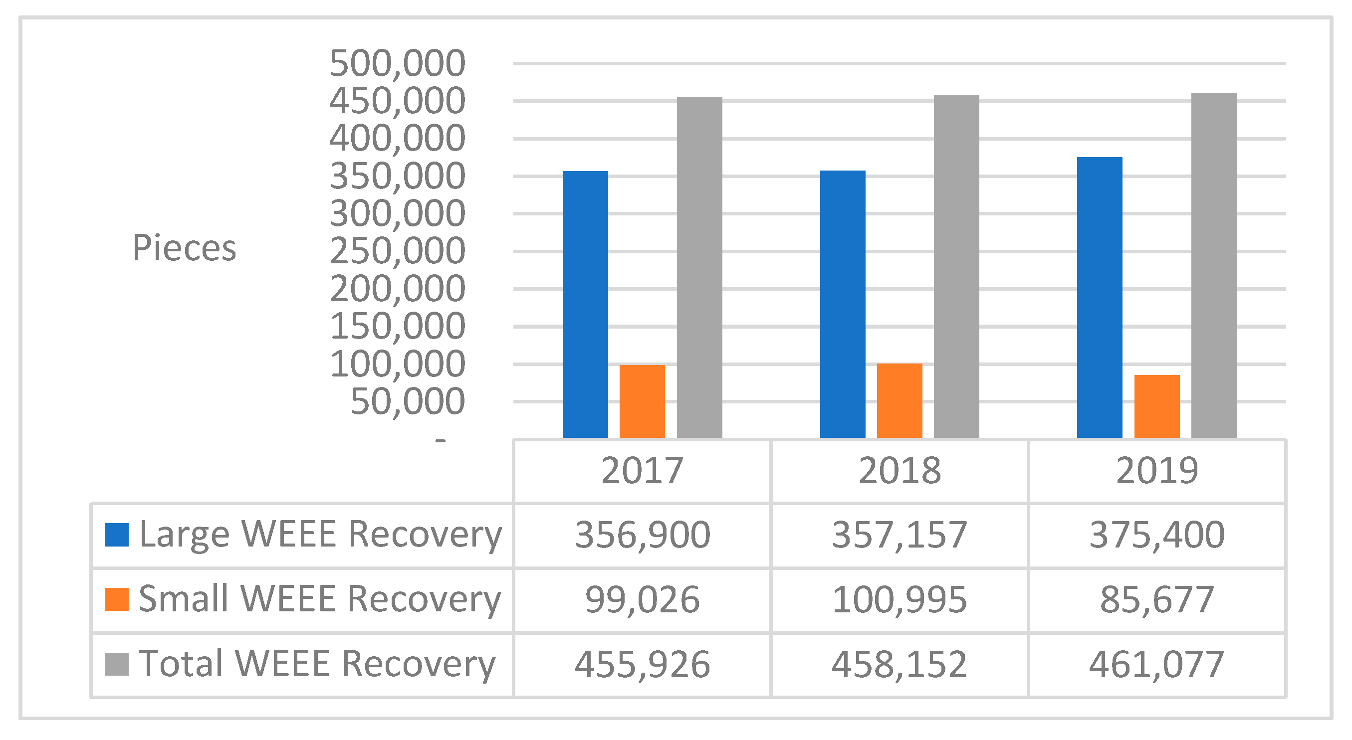
From 2017 to 2019, the statistics of return amount of large and small waste electronic products of J company are shown in Figure 6 and the total number in three years has reached 1,375,155. Large and small pieces are divided by product volume. For example, large waste electronic products include refrigerators and televisions, while small waste electronic products refer to mobile phones and batteries. All these waste electronic products are recycled through 51 primary recycling sites.

As depicted in Figure 6, it is found that WEEE product return from 2017 to 2019 tends to be stable, in line with the second-order random hypothesis. Therefore, in this case study, the model proposed in this paper is mainly based on the measured data of return from 2017 to 2019 (36 months in total).

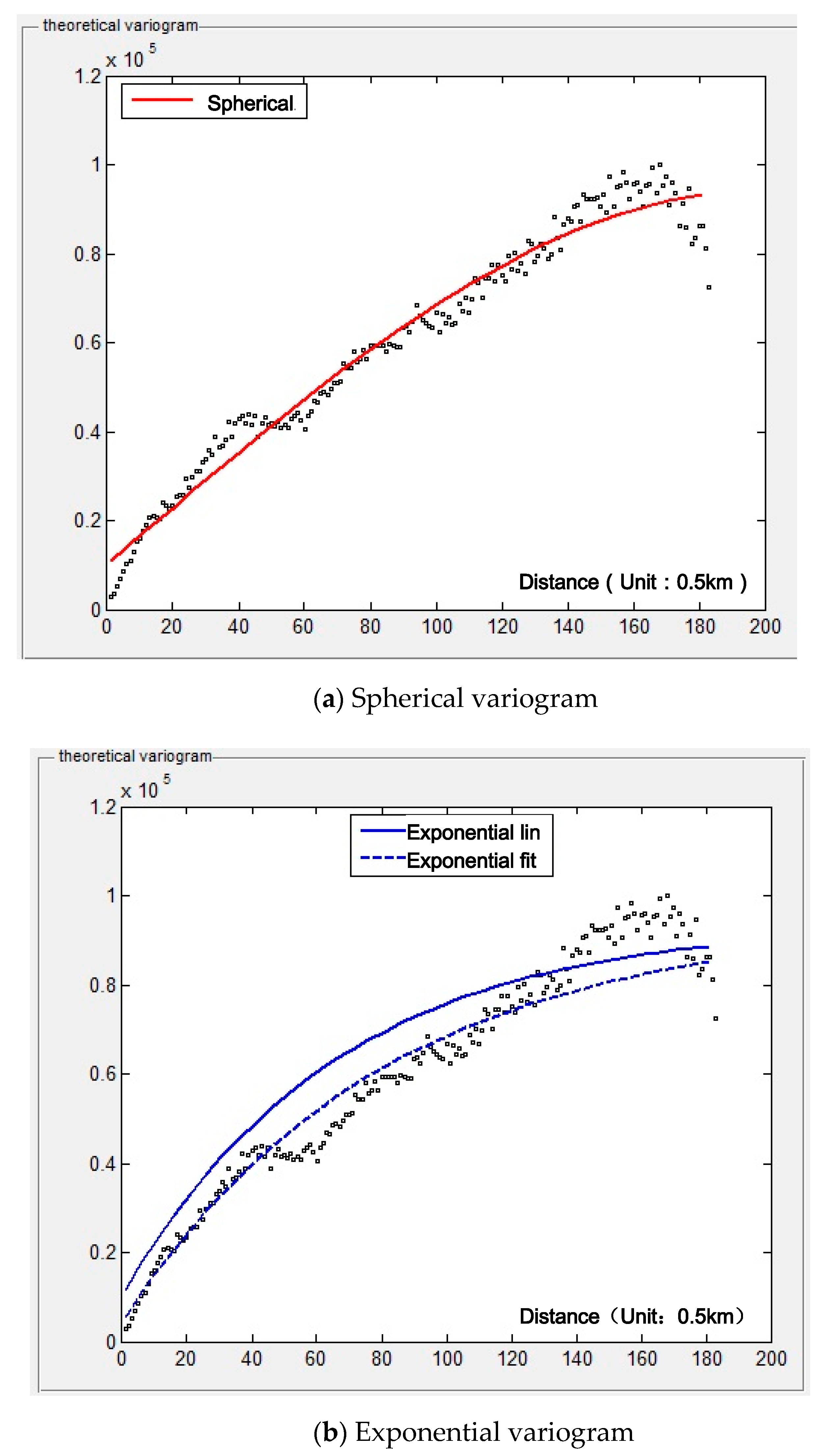
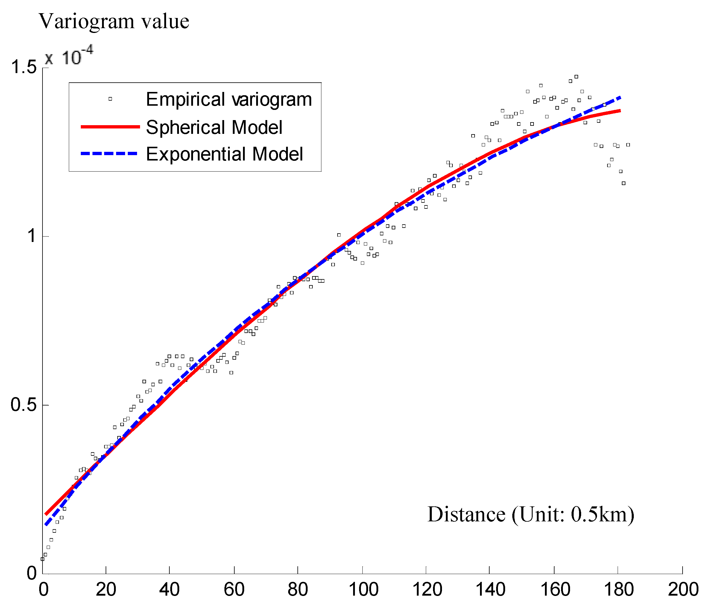
According to Simulation conclusion 2, for the recycling of WEEE with spatial correlation, the prediction value of Kriging method based on exponential variogram is theoretically optimal and the error is minimum. Therefore, in this case study, exponential variogram is mainly used to analyze the spatial structure of return amount. The fitting results of the exponential variogram of return amount are shown in Figure 7, and the quantitative calculation results are shown in

Table 5. Quantitative analysis results of exponential variogram of WEEE return for J company.

No. of Sites	Variogram	$\mathbf{Sill}({\mathit{C}}_0+{\mathit{C}}_1)$	$\mathbf{Nugget}\left({\mathit{C}}_0\right)$	Structural Variance Ratio
51	Exponential	1.4141 × 10−4	0.148 × 10−4	90.39%

.

Case conclusion 1: As can be seen from Figure 7, the correlation length of WEEE return amount of J company from 2017 to 2019 is about 90 km, that is, if the distance exceeds 90 km, the correlation will decrease quickly. This phenomenon is consistent with the actual situation. The distance from Baoshan District in the north of Shanghai to Hangzhou Bay in the southernmost Jinshan District of Shanghai is about 90 km. If this distance is exceeded, the two recycling sites will be located in two different administrative areas (such as Shanghai and Kunshan City of Jiangsu Province). Due to the great differences in regional policies, the spatial correlation of the two recycling sites will decrease rapidly.

Case conclusion 2: It can be seen from Figure 8 that for company J with 51 primary recycling sites, the structural variance ratio is 90.39% when using exponential variogram. Meanwhile, the structural variance ratio of the sample with 50 recycling sites using exponential variogram in the simulation example is 89.41%. The simulation results are basically consistent with the measured data.

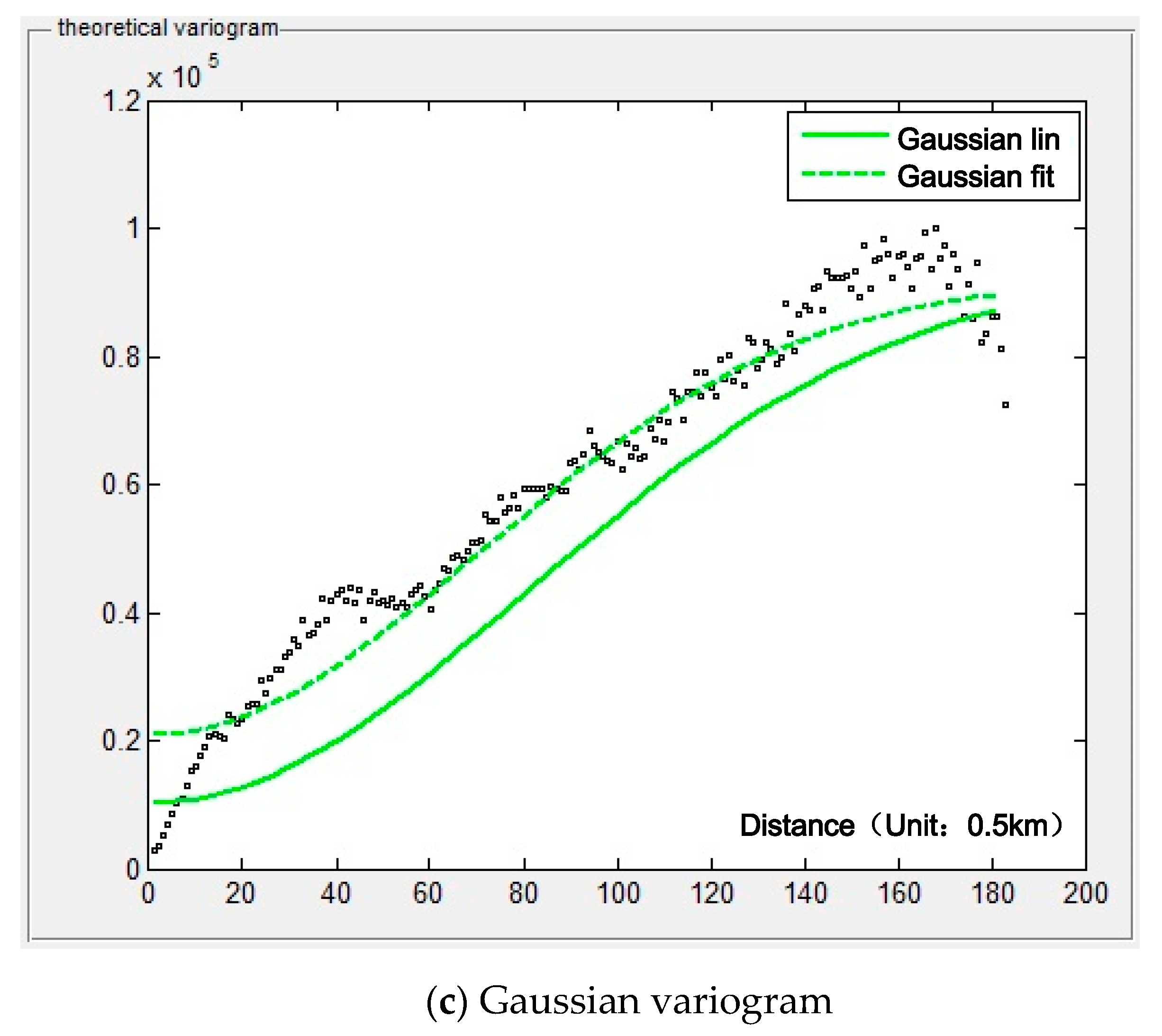
In order to further analyze and compare the fitting performance of the different variograms, the measured data are used for comparative analysis, and the results are shown in Figure 8.

Case conclusion 3: According to the fitting results of the measured data, both exponential variogram and spherical variogram are better than the Gaussian variogram, which verifies the simulation results.

The actual WEEE return of J company in 36 months is divided into two parts. The data of first 24 months are used as training samples, and the data of last 12 months are used as test samples. The Kriging model of exponential variogram is used to predict the return in the next 12 months. The final evaluation of the prediction results is shown in

Table 6. Quantitative analysis results of exponential variogram of WEEE return for J company.

No. of Sites	Variogram	PEP	SDPE
51	Exponential	1.43%	0.04578

.

Case conclusion 4: The prediction error percentage of the Kriging model using exponential variogram is 1.43%, and the standard deviation is 0.04578. The prediction error is close to the total error (1.21%) in the simulation example. Generally speaking, the prediction performance of this paper based on the Kriging model is acceptable.

5. Conclusions

In order to deal with environmental legislation and ease the pressure of resources, logistics management has evolved from a linear model to a higher level closed-loop mode including reverse logistics. Due to the uncertainty of WEEE return, the prediction of waste product return in WEEE reverse logistics has always been a difficult problem for industry and academia. From a new perspective, considering the spatial correlation of WEEE recycling sites, this paper introduces the spatial statistical Kriging method to establish the spatial model of reverse logistics return prediction, which provides a new method and theoretical basis for the return prediction of WEEE of reverse logistics.

According to the results of Monte Carlo simulation and J company’s case, the spatial model based on the Kriging method can accurately predict the WEEE return amount, and the total prediction error percentage is 1.21% and 1.43%, respectively, which indicates good accuracy of the proposed model.

Three variograms commonly used in simulation examples are utilized to analyze the spatial correlation structure of WEEE return. The prediction error percentage of exponential variogram is 0.77%, less than those of spherical variogram (1.01%) and Gaussian variogram (1.85%). Among the three types of variograms, the exponential variogram achieves better prediction results. Therefore, the exponential variogram is recommended when considering the spatial correlation of WEEE return. The case study of J company also proves that the exponential variogram has achieved better results.

For the WEEE return system with different number of recycling sites, the number of recycling sites in the simulation example ranges from 10 to 100. For a practical reverse logistics WEEE return system, the number of return sites is basically covered. There is no significant prediction error fluctuation when using this model, which proves the universal applicability of the proposed method.

In the case of J company and the simulation example, there is a correlation length a for the WEEE return system. When the distance between any two sites is less than a, there is a correlation between the return amounts of different sites. With the increase of the distance, the spatial correlation weakens, and when the distance is greater than a, the spatial correlation disappears. The simulation results show that the variation distance is about 90 km by using three commonly used variograms, which provides a useful reference for the spatial correlation analysis of WEEE reverse logistics recycling system.

For future work, there are two main aspects worthy of further study. On the one hand, due to the technical innovation and policy incentives, the return amount might increase greatly and sharply. Once the return amount does not meet the second-order randomness assumed in this paper, a new theoretical method needs to be deduced and verified. On the other hand, it is worth establishing a mathematical model which considers both temporal and spatial correlation of the return amount. It might be difficult in theoretical derivation, but it is of great significance for the actual return prediction of WEEE reverse logistics.