Article

Franken-CT: Head and Neck MR-Based Pseudo-CT Synthesis Using Diverse Anatomical Overlapping MR-CT Scans

by
Pedro Miguel Martinez-Girones
1,
Javier Vera-Olmos
1,
Mario Gil-Correa
1,
Ana Ramos
2,
Lina Garcia-Cañamaque
3,
David Izquierdo-Garcia
4,
Norberto Malpica
1 and
Angel Torrado-Carvajal
1,4,*
1
Medical Image Analysis and Biometry Laboratory, Universidad Rey Juan Carlos, 28933 Madrid, Spain
2
Department of Radiology, Hospital Universitario HM Puerta del Sur, HM Hospitales, 28938 Madrid, Spain
3
Department of Nuclear Medicine, Hospital Universitario HM Puerta del Sur, HM Hospitales, 28938 Madrid, Spain
4
Athinoula A. Martinos Center for Biomedical Imaging, Massachusetts General Hospital and Harvard Medical School, Boston, MA 02129, USA
*
Author to whom correspondence should be addressed.
Appl. Sci. 2021, 11(8), 3508; https://doi.org/10.3390/app11083508
Submission received: 31 December 2020 / Revised: 30 March 2021 / Accepted: 8 April 2021 / Published: 14 April 2021
(This article belongs to the Special Issue PET Imaging with Deep Learning)

Abstract

:

Featured Application

The Franken-CT approach allows synthesizing pseudo-CT images from using diverse anatomical overlapping MR-CT datasets as a potential application in PET/MR attenuation correction.

Abstract

Typically, pseudo-Computerized Tomography (CT) synthesis schemes proposed in the literature rely on complete atlases acquired with the same field of view (FOV) as the input volume. However, clinical CTs are usually acquired in a reduced FOV to decrease patient ionization. In this work, we present the Franken-CT approach, showing how the use of a non-parametric atlas composed of diverse anatomical overlapping Magnetic Resonance (MR)-CT scans and deep learning methods based on the U-net architecture enable synthesizing extended head and neck pseudo-CTs. Visual inspection of the results shows the high quality of the pseudo-CT and the robustness of the method, which is able to capture the details of the bone contours despite synthesizing the resulting image from knowledge obtained from images acquired with a completely different FOV. The experimental Zero-Normalized Cross-Correlation (ZNCC) reports 0.9367 ± 0.0138 (mean ± SD) and 95% confidence interval (0.9221, 0.9512); the experimental Mean Absolute Error (MAE) reports 73.9149 ± 9.2101 HU and 95% confidence interval (66.3383, 81.4915); the Structural Similarity Index Measure (SSIM) reports 0.9943 ± 0.0009 and 95% confidence interval (0.9935, 0.9951); and the experimental Dice coefficient for bone tissue reports 0.7051 ± 0.1126 and 95% confidence interval (0.6125, 0.7977). The voxel-by-voxel correlation plot shows an excellent correlation between pseudo-CT and ground-truth CT Hounsfield Units (m = 0.87; adjusted R2 = 0.91; p < 0.001). The Bland–Altman plot shows that the average of the differences is low (−38.6471 ± 199.6100; 95% CI (−429.8827, 352.5884)). This work serves as a proof of concept to demonstrate the great potential of deep learning methods for pseudo-CT synthesis and their great potential using real clinical datasets.

1. Introduction

In the last 20 years, the interest on synthetizing pseudo-Computerized Tomography (pseudo-CT) images from Magnetic Resonance (MR) images using computer vision and machine learning techniques has been increasing consistently alongside the adoption of hybrid Positron Emission Tomography/Magnetic Resonance (PET/MR) scanners and the improvement in external radiation therapies [1,2,3]. The first approaches used traditional image processing and machine learning strategies, such as segmentation-based methods [4,5,6,7], atlas-based methods [8,9,10,11,12,13,14], or learning based methods [15,16,17].
These approaches present several disadvantages, such as the need of an accurate spatial normalization to a template space, the assumption of mostly normal anatomy, or the problem of accommodating a large amount of training data. These problems have been solved in the last few years with the advent of new techniques based on Convolutional Neural Networks (CNNs). The use of CNNs has also improved the quality of the result while reducing the time needed for synthesizing a pseudo-CT. According to our knowledge, the first approach that adopted deep learning to generate a pseudo-CT from an MRI scan was presented by Xiao Han et al. [18]. This work proposed a CNN that used a U-net architecture performing 2D convolutions [19]. The network received axial slices from a T1-weighted volume of the head as input and tried to generate the corresponding slices from a registered CT scan. Their architecture incorporated unpooling layers in the up-sampling steps of the U-net and Mean Absolute Error (MAE) as loss function. Their results were compared to an atlas-based method [20], obtaining favorable results in accuracy and computational time (close to real-time). Later, the work of Fang Liu et al. [21] explored a similar architecture to generate a segmentation of air, bone, and soft tissue instead of generating the continuous pseudo-CT, also using a set of 3D T1-weighted head volumes. In this case, they incorporated a nearest-neighborhood interpolation in the up-sampling steps of the U-net. Additionally, as they were classifying instead of regressing, they employed a multi-class cross-entropy loss metric, which is usually easier to optimize than the L1 or L2 error. Their results were compared with the capability of their segmentation to reconstruct PET images against the reconstruction using Dixon base Attenuation Correction (AC) images. The deep learning approach performed better and took less than 0.5 min to generate the pseudo-CT segmentation.
In contrast, our work by A. Torrado-Carvajal et al. [22] proposed a 2D U-net architecture with transposed convolutions as up-sampling layer based only on Dixon images. In this case, we utilized the Dixon-VIBE images from the Pelvis as input to the network to generate their corresponding pseudo-CT. Therefore, the input to the network was composed by four channels corresponding to the four values of the Dixon image. This proposal generated a whole pseudo-CT volume in around 1 min.
Other works made use of more sophisticated networks architectures and pipelines for training. The work by D. Nie [23] proposed a 3D neural network with dilated convolutions to avoid the use of pooling operations. They also explored the advantages of residual connections [24] and auto-context refinement [25]. For training, they employed an adversarial network that tried to differentiate between real CTs and pseudo-CTs [26]. They used 3D patches from T1 volumes of head and pelvis as input and compared their results against traditional methods such as atlas registration, sparse representation, and random forest with auto-context. Their approach outperformed all these methods. On the other hand, a similar approach was proposed by H. Emami et al. [27] which trained a 2D CNN that incorporated residuals and an adversarial strategy for training.
All these recent strategies, including both atlas-based methods and neural networks, relay on databases to generate a dictionary or to train a model. These databases are composed by complete MR volumes and their corresponding CT volumes acquired for a certain field of view (FOV) of interest. However, finding MR-CT pairs that match those requirements—and including spatial resolution and contrast constrains required to generate those training datasets—in retrospective clinical studies is usually difficult, limiting the flexibility and generalizability of these databases. On the other hand, whole-body acquisition strategies are gaining importance in early diagnosis, staging, and assessment of therapeutic response in oncology [28].
In this scenario, while MR whole-body acquisition has accelerated its deployment and acceptance in clinical practice, in the acquisition of CT images, the FOV is generally reduced in order to lower the radiation dose to the patient. Thus, to create highly flexible and generalizable atlases to train our algorithms in a real clinical setting, we should be able to work with datasets containing lower resolution but bigger FOV MR images alongside low dose and reduced FOV CT images.
In this work, we propose a method based on the idea of modality propagation using MR-CT atlases described in preceding developments [11,29] and a deep learning architecture approach inspired on our previous work [22]. However, our database is composed by head and neck MR images and local portions of CT including the brain, paranasal sinuses, facial orbits, and neck studies. Additionally, the deep learning architecture presented here incorporates novel state of the art techniques. With this work we demonstrate that constructing and using incomplete databases still enables accurate results without major limitations, as Deep Learning methods have the potential to be used with this kind of datasets if certain steps and correction are performed on the pipeline.

2. Materials and Methods

Our proposed Franken-CT approach for pseudo-CT synthesis can be divided into two main steps: (1) a non-overlapping and non-parametric atlas generation, (2) the implementation of the modality propagation for pseudo-CT synthesis algorithms. The details about both steps are described below.

2.1. Franken-Computerized Tomography (Franken-CT) Approach

Typically, modality propagation schemes proposed in the literature rely on complete corresponding atlases—volumes acquired with the same FOV—to the input volume. However, CTs are usually acquired in a reduced FOV to decrease patient ionization and acquisition time in the clinical practice. Thus, we base our work on a diverse anatomical overlapping MR-CT atlas. This new atlas may contain complete MRI volumes but only different anatomical overlapping CT scans, as shown in Figure 1.

2.2. Magnetic Resonance-Computerized Tomography (MR-CT) Datasets

2.2.1. Training Dataset

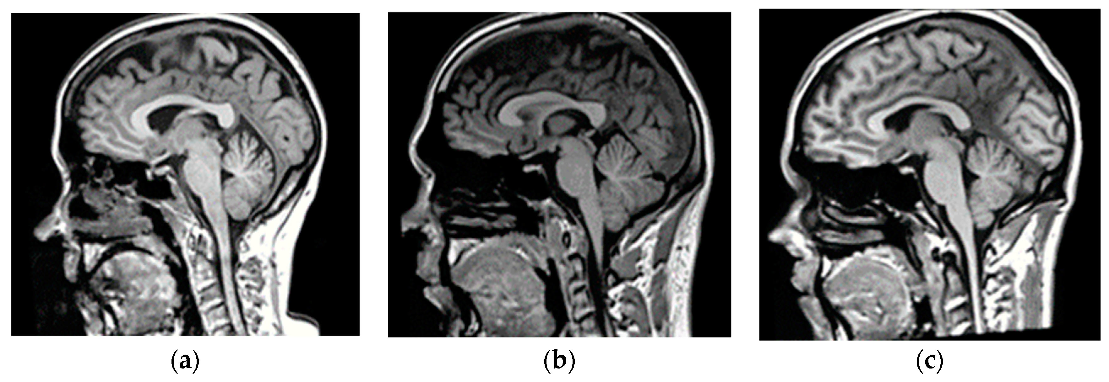
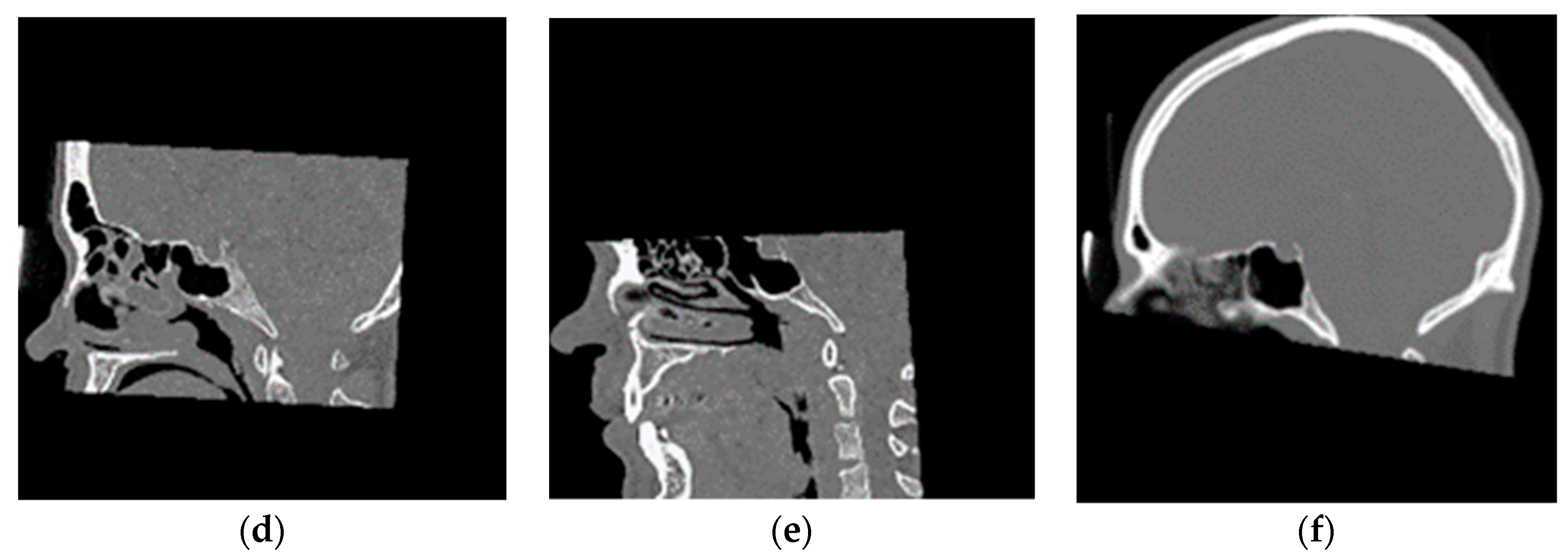
Scans of 15 subjects (mean age, 58.2 ± 18.1 years old; range, 25–80 years old; 9 females/6 males) that underwent both MR and CT imaging were selected. MR images were acquired in the sagittal plane to include head and neck in the FOV while CT images focused on local FOVs including brain, paranasal sinuses, facial orbits, or neck studies. MR T1-weighted sequences differed depending on the MR scanner (images were acquired at different field strengths and in different scanner models). Additionally, images were acquired using different coils with different amount of channels. Regarding CT images, all subjects underwent CT examinations depending on their pathologies on an Aquilion Prime CT scanner (Toshiba). Table 1 summarizes the demographic details for all subjects included in the training dataset as well as their corresponding MR and CT scans vendors and models. Extended details are included in Table A1 in Appendix A. Figure 2 shows representative images from different subjects included in the training dataset.

2.2.2. Validation Dataset

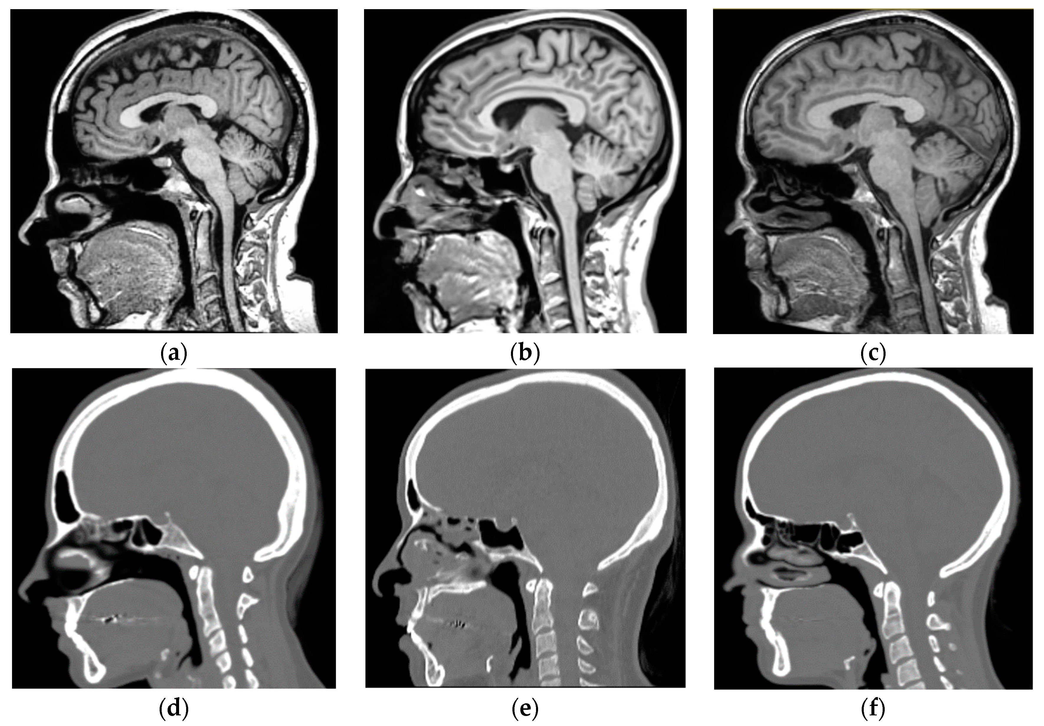
Scans of 6 subjects (mean age, 39.5 ± 23.42 years old; range, 21–83 years old; 4 females/2 males) that underwent both MR and CT head and neck imaging were selected to validate the Franken-CT approach. Figure 3 shows representative images from different subjects included in the validation dataset. Table 2 summarizes the demographics and technical details of the MR and CT imaging protocols for all subjects included in the validation dataset. Extended details are included in Table A2 in Appendix A.

2.2.3. Datasets Preprocessing

Image preprocessing was carried out to normalize all the images in the dataset to the same intensity value range and in the same spatial distribution, including:
  • MRI bias correction on the anatomical T1-weighted images (N4ITK MRI Bias Correction, 3D Slicer) to correct for inhomogeneities caused by subject-dependent load interactions and imperfections in radiofrequency coils.
  • Resampling of MR and CT images to an isotropic 1 mm space was performed (Resample Scalar Volume, 3D Slicer) to set a common resolution space for all images ((271, 271, 221) pixels) and avoid information loss in the following steps.
  • Intra-patient rigid registration to align each MR-CT pair. The method consists of an initial manual registration using characteristic points (Fiducial Registration Wizard, 3D Slicer), an automatic rigid registration step (General Registration Brains, 3D Slicer), and a manual adjustment of the registration (Transforms, 3D Slicer). This is a crucial step and guarantees the correspondence between each anatomical point of both image techniques.
  • Reslicing and crop all MR and CT images to a reference image (Resample Image Brains, 3D Slicer) to ensure the same matrix size prior training our network.
  • MR histogram matching (MATLAB, MathWorks Inc., Natick, MA, USA) to normalize intensity values between images, especially for those images acquired with different scanners.
  • CT intensity normalization from −1024 to 3071 Hounsfield Units (HU) (MATLAB, MathWorks Inc.) to ensure a representation of 4096 gray levels, as defined by HU.
  • MR-CT image information matching (MATLAB, MathWorks Inc.) to ensure there is no MR or CT information in areas where one of the modalities is out of the other, so as to ensure that the same anatomical area is represented in both MR and CT.

2.3. Pseudo-CT Synthesis

In this work, we propose a Deep Learning architecture based on a U-net architecture that has been used in various approaches before [18,21,22]. The U-net architectures have been implemented in different ways, nevertheless it is always based on a progressive down-sampling of the feature maps followed by a step of up-sampling to generate the final output. Generally, during the down-sampling phase, several convolution filters and sub-sampling operations, such as max-pooling or convolutions with stride, are employed. On the other hand, during the up-sampling phase, the feature maps are up-sampled using operations, such as unpooling or transposed convolutions. Additionally, before each sub-sampling operation in the down-sampling phase, the feature maps are usually connected to their counterpart in the up-sampling phase with the same size to improve the quality of the output.
Considering this, we have redesigned the architecture of the U-net to incorporate residual operations and convolutions with dilation. These operations have been successfully employed for image classification [24] and image segmentation [30]. Figure 4 depicts an overview of our proposed U-net architecture incorporating these strategies.
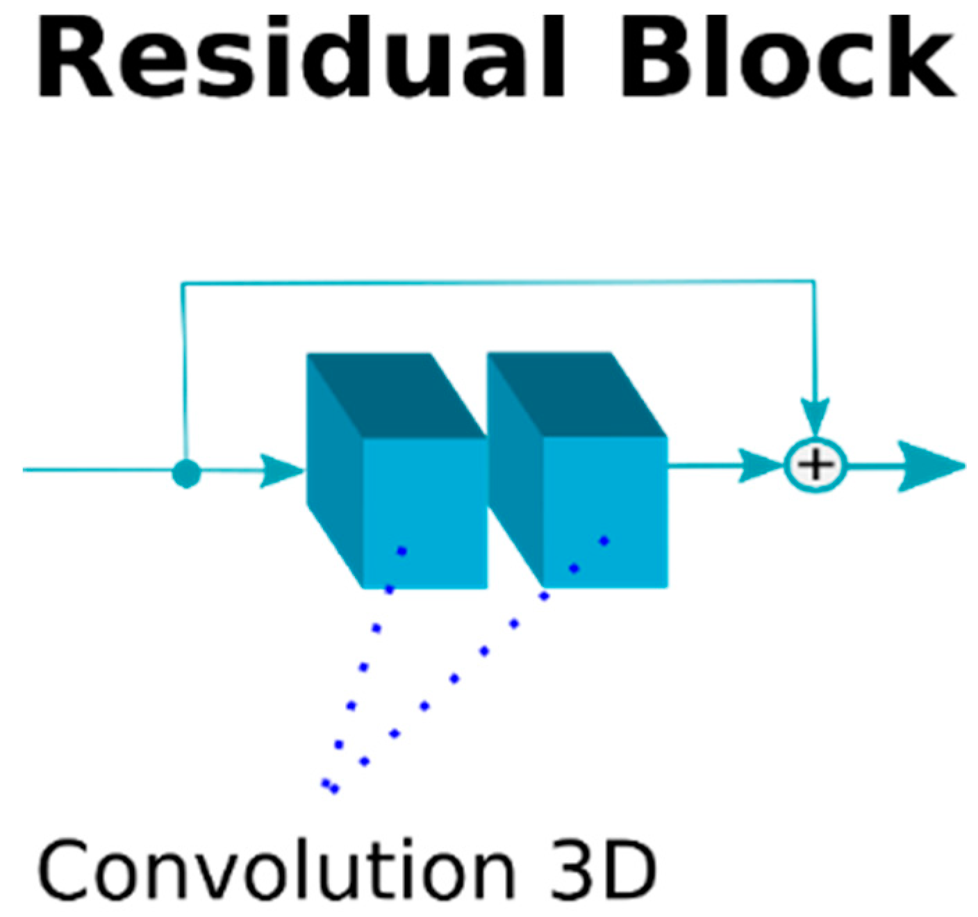
The residual operation consists in a shortcut that adds the feature maps generated by a previous layer to the result of a layer ahead. Figure 5 depicts the residual operation used inside each blue box in our implementation depicted in Figure 4. The residual operation has demonstrated to be very effective to increase the depth of neural networks without a degradation of the results [24]. Therefore, we performed a residual shortcut after every two convolutions during the down-sampling and the up-sampling phase. The convolutions with dilation conform the convolution called “Atrous” [30], which entails the use of kernels that are not applied directly on neighborhoods in the feature maps but on values that are separated by a few neighbors. Figure 6 gives a visual explanation of the Atrous convolution. We started with a filter with dilation 1, which means a regular convolution filter, but after every two convolutions (i.e., after each residual block) we increased the dilatation parameter by 1 and reset it after every sub-sampling or up-sampling operation.
As for our concrete implementation of the sub-sampling and up-sampling operations during the U-net phases, we decided to use convolutions with stride 2 as sub-sampling and transposed convolutions as up-sampling operations. Depending on the stage of the sub-sampling and the up-sampling, a different number of residual blocks are performed, increasing them as the feature maps are down-sampled, and reducing the amount of blocks when the feature maps are up-sampled. Finally, after every convolution a batch normalization is performed and then a ReLU activation function is applied to generate the feature maps.

2.4. Training and Reconstruction

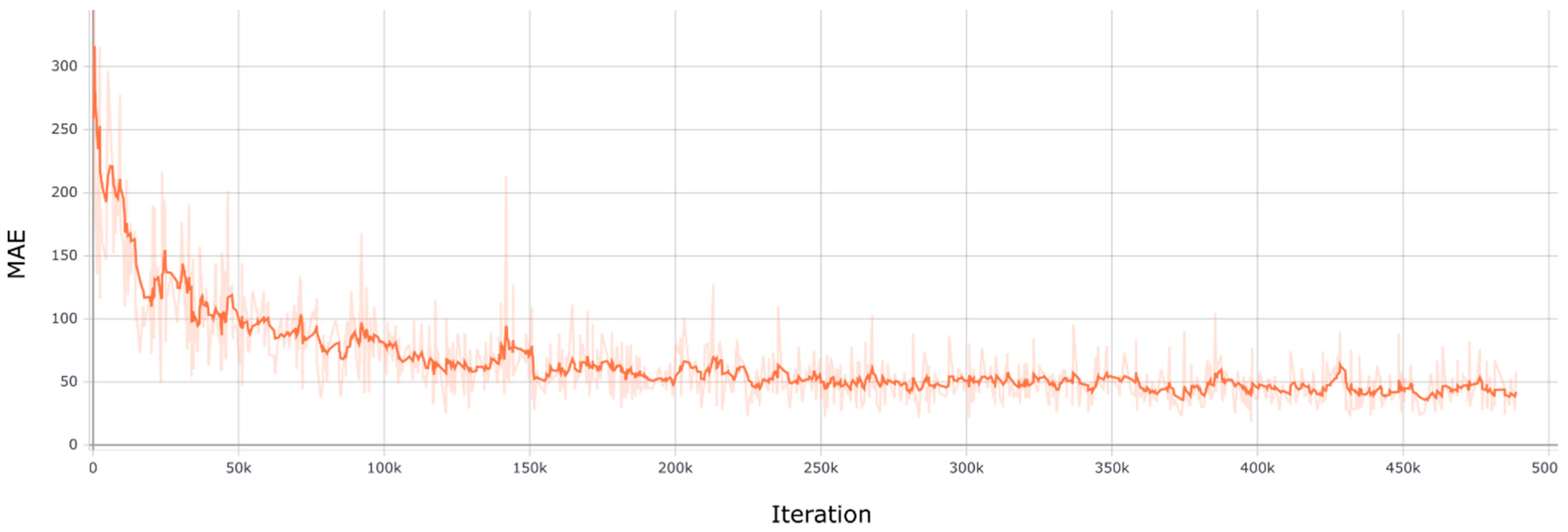
As input for the network, we used 3D patches of shape 32 × 32 × 32 and we performed 3D convolutions with 3 × 3 × 3 kernels. As loss function, we employed Mean Absolute Error and Adam optimization with a learning rate of 10−4. The mini-batch size was set to 8 patches and we performed random rotations to the patches during training for data augmentation. To train the network, we generated a database using all the training volumes to obtain 3D patches with stride 8. We trained the model until convergence, which happened after 25 epochs at ~45 MAE; it took around 90 h using a Nvidia RTX 2080Ti. To reconstruct a whole pseudo-CT volume, we divided every input 3D volume in cubes with shape 32 × 32 × 32 using stride 16 in every direction to use them as input in the trained network. However, to compose the pseudo-CT, we used only the inner 16 × 16 × 16 cube of every 3D patch synthetized to improve the quality of the reconstruction and avoid artifacts in the border of each patch. The whole reconstruction of a pseudo-CT volume takes around one minute in the Nvidia RTX 2080Ti.

2.5. Evaluation

The zero-normalized cross correlation (ZNCC) similarity metric, Mean Absolute Error (MAE), Structural Similarity Index Measure (SSIM), as well as the Dice coefficient for bone class were computed to quantitatively measure the quality of the synthesized pseudo-CT volumes compared with the ground-truth CT volumes and thereby checking if there is an overlap of tissues, following Equations (1)–(4):
ZNCC = 1 N x , y , z pCT x , y , z μ pCT CT x , y , z μ CT σ pCT σ CT
MAE = 1 N x , y , z pCT x , y , z CT x , y , z
SSIM pCT , CT = 2 μ pCT μ CT + c 1 2 σ pCT , CT + c 2 μ pCT 2 + μ CT 2 + c 1 σ pCT 2 + σ CT 2 + c 2
where x, y, and z are the three-dimensional image dimensions; N is the total amount of voxels; pCT x , y , z and CT x , y are the pseudo-CT and ground-truth CT voxel values for a given (x,y,z) position, respectively; μ pCT and μ CT are the mean HU pseudo-CT and ground-truth CT images, respectively; σ pCT and σ CT are the standard deviation for the pseudo-CT and ground-truth CT images, respectively, and σ pCT , CT is the joint standard deviation; and c 1 = k 1 L 2 ,   c 2 = k 2 L 2 are two variables to stabilize the division with weak denominator depending on L= dynamic range of pixel values (typically 2#bits per pixel − 1), k 1 = 0.01 and k 2 = 0.03 by default.
The distance range of ZNCC is the interval (−1, 1) (1 for perfect direct correlation, −1 for perfect inverse correlation, and 0 for non-correlation).
D I C E b o n e = 2   M pCT M CT M pCT + M CT
where M pCT and M CT are the mask segmentations obtained by thresholding Hounsfield Units values for bone tissues in the pseudo-CT and ground-truth CT, respectively.
Mean ± standard deviation (SD), as well as the 95% confidence interval (CI) for ZNCC, MAE, SSIM, and Dice were computed.
Voxel-by-voxel analyses were performed to determine differences in synthesized pseudo-CT compared to the ground truth CT. Voxel-by-voxel correlation plots, Bland–Altman plots, bias, and variability Pearson correlation coefficients were calculated for comparisons. Statistical significance was considered when the p value was lower than 0.01.

3. Experimental Results

3.1. Convolutional Neural Network (CNN) Results

Figure 7 depicts the loss function during training and Figure 8 shows three planes of how a representative resulting pseudo-CT evolves during training.

3.2. Franken-CT Approach Results

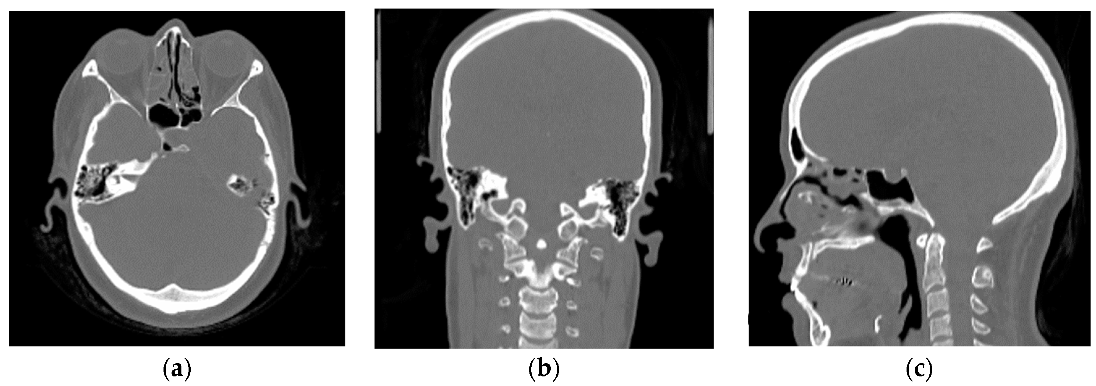
Figure 9 shows the MR and CT images as well as the pseudo-CT obtained using our Franken-CT method, demonstrating quite promising correlation between pseudo-CT and CT, considering the relatively small training dataset. Visual inspection of the results showed the high quality of the resulting pseudo-CT and the robustness of the Franken-CT method, which is able to capture the details of the bone contours and spikes in non-smooth areas such as the sinuses and the cervical vertebrae. The shape of the skull was estimated correctly despite synthesizing the resulting image from knowledge obtained from images acquired with a completely different FOV. Neck areas show limited detail in resolution compared to upper brain areas, probably due to the difference in the number of atlases for those specific areas. Moreover, certain differences can be noticed in nasal sinus cavity, mastoid cells and in air cavity delineation, possibly due to the complexity of these anatomies. Overall, the image texture is a bit smoother in the pseudo-CT compared to ground-truth CT.
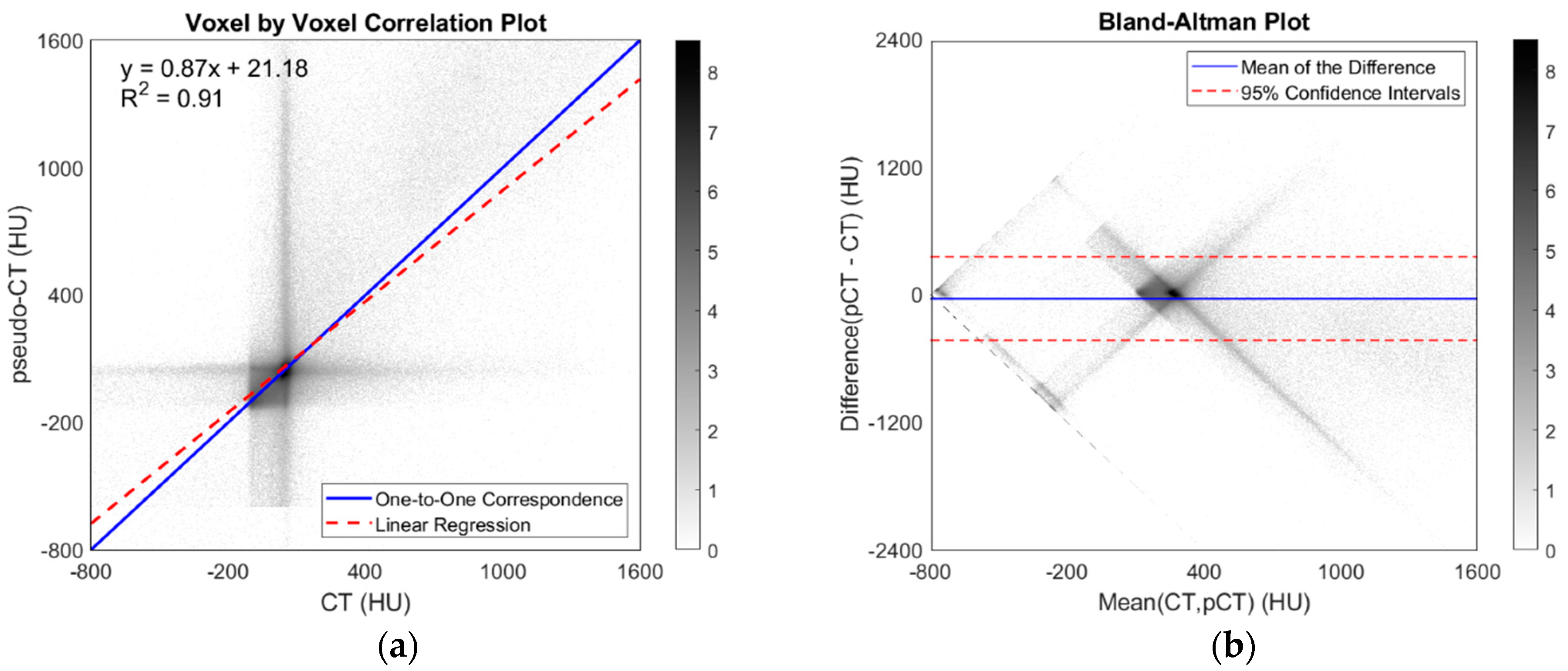
The experimental ZNCC was 0.9220 ± 0.0255 and 95% confidence interval (0.9010, 0.9430); the experimental Mean Absolute Error (MAE) was 73.9149 ± 9.2101 HU and 95% confidence interval (66.3383, 81.4915); the Structural Similarity Index Measure (SSIM) was 0.9943 ± 0.0009 and 95% confidence interval (0.9935, 0.9951); and the experimental Dice coefficient for bone tissue was 0.7051 ± 0.1126 and 95% confidence interval (0.6125, 0.7977). Moreover, the voxel-by-voxel correlation plot as well as the Bland–Altman plot between pseudo-CT and CT were computed for all test participants (Figure 10). The correlation plot showed an excellent correlation between pseudo-CT Hounsfield Units and ground truth CT Hounsfield Units (m = 0.87; adjusted R2 = 0.91; p < 0.001). The Bland–Altman plot showed that the average of the differences was low (−38.6471 ± 199.6100; 95% CI (−429.8827, 352.5884)); the difference between methods tended to decrease as the average increased, accumulating the error in voxels around 0 HU.

4. Discussion

The generation of precise pseudo-CT images, and thus the production of accurate AC maps, is a basic step for PET/MRI quantification. Several approaches have been proposed in the literature providing exciting results, but most of them focus on specific areas of the body or use specific acquisitions in order to try those methods. However, the reality in a clinical setting shows the trend to minimize FOVs in CT acquisitions, making it difficult to create high quality atlas to be used for these applications. Additionally, there is a tendency to extend FOVs to increase the amount of multimodal information and to move to whole-body applications in PET/MR.
In this work, we proposed the use of DL to acquire knowledge from diverse anatomical areas, from an overlapping MR-CT atlas, and use that information to be able to synthesize a pseudo-CT volume corresponding to a bigger FOV image. Thus, we demonstrated how using different images including brain, paranasal sinuses, facial orbits, and neck studies can lead to the successful generation of continuous head and neck pseudo-CTs. For reproducing this achievement through a new dataset with the Franken-CT approach, all the specific preprocessing steps described previously in the Materials and Methods section need to be followed every time.
Our results are in line with those recently described by other authors but using complete and/or dedicated atlases. The qualitative (Figure 9) and quantitative (Figure 10) image quality analyses performed showed that the CT and the pseudo-CT obtained with our Franken-CT method are very similar. On the one hand, the visual inspection shows a good correspondence between both images but a limited detail in the neck region, nasal sinus cavity, mastoid cells, and air cavity delineation. This fact is possibly due to the higher complexity of those regions and the limited amount of neck scans in the train atlas; increasing the number of such MR-CT pairs in the training dataset should improve the resulting pseudo-CTs, as previously demonstrated in state-of-the-art investigations about the effect of training dataset sizes [31]. However, despite these limitations, visual comparison of our synthesized pseudo-CT images with those previously reported in previous works shows our method provides better images than most classical and recently proposed deep-learning methods in the literature [14,32,33]. On the other hand, the high ZNCC values indicate that our method can accurately approximate the patient-specific CT volume, despite using an atlas composed of diverse anatomical overlapping MR-CT scans. Previously described patch-based pseudo-CT synthesis methods reported an experimental ZNCC of 0.9349 ± 0.0049 for a whole head and neck atlas including 18 MR-CT datasets [11,29], which is very similar to the experimental ZNCC of 0.9220 ± 0.0255 achieved in this work. Likewise, other patch-based methods of the state-of-the-art provide average ZNCC of 0.91 ± 0.03 and mean MAE of 125.46 ± 24.45 HU [34], in contrast with the results presented in this work of average ZNCC and the experimental MAE of 73.9149 ± 9.2101 HU. Works based in CNN report average SSIM of 0.92 ± 0.02 and mean MAE of 75.7 ± 14.6 [35] in comparison with average SSIM of 0.9943 ± 0.0009 and mean MAE achieved by our Franken-CT approach. In the evaluation of overlapping in bone tissues other authors reported a Dice coefficient of 0.73 ± 0.08 [36] which is in line with the average Dice coefficient of 0.7051 ± 0.1126for bone overlap reported in this work, quite promising but probably impacted due to the neck region results discussed previously. These facts suggest that (i) the use of an atlas composed of diverse anatomical overlapping MR-CT scans can produce similar results to those reached by complete datasets and, (ii) deep learning methods enable extracting more features and information than classical methods. Recently, works on deep-learning pseudo-CT synthesis reported a Pearson correlation of up to 0.943 ± 0.009 using a similar architecture to the one presented in this work [37]; again, this demonstrates: (i) the great potential of deep learning methods to extract features and information and, (ii) the increased performance of architectures including residual operations to avoid the degradation in the feature maps generated. Additionally, the correlation and the Bland–Altman plots (Figure 10) suggest this method leads to very accurate results, and in line with those previously reported in the literature, despite minor errors mainly accumulated in voxels between 25 and 125 HU (banding artifacts in the correlation and Bland–Altman plots). We further investigated this issue and found that most of these mislabeled voxels are predominantly located in image boundaries/edges and ears (due to slight differences between MR and CT), air-filled cavities, and dental implants, as could be appreciated in Figure 9. Despite the weaknesses presented, as the synthesized image is not going to be used for diagnostic reading performed by radiologists, but just for PET attenuation correction, the level of detail of the pseudo-CT does not need to be equivalent to a real acquired CT. In this specific context, a minor loss in spatial resolution is acceptable, as the inherent PET resolution is lower than CT or MR spatial resolution.
The approach presented in this work could be of great potential for tasks where the skull estimation and/or the pseudo-CT computation is needed, such as PET/MR attenuation correction and radiotherapy planning where MR-CT datasets are usually limited, leading to larger and highly flexible and generalizable atlases.
This method could be adapted to real clinical scenarios as training these algorithms requires long times but their use and application for synthesis is very fast, synthesizing a complete pseudo-CT volume in a similar time to that needed to acquire an actual CT scan. Additionally, our technique could, in theory, be applied in other regions of the body, potentially allowing for whole-body pseudo-CT synthesis using atlases designed with the same hypothesis. Further research will be aimed in that direction.
Our study presents several limitations. First, our training set was relatively small, which has a bigger effect when using the described Franken-CT approach compared to traditional methods. this is due to the fact that we only have a subset of subjects including information for specific anatomical areas, decreasing the effective N of the atlas. Additionally, our atlas contained subjects biased towards high ages. However, our approach proves that not discarding reduced FOV images allows producing accurate results; therefore, using as many datasets as available to increase the number of datasets and produce larger databases for DL training will allow to train more generalizable CNNs than those reported previously. Further improvement of the current model could be achieved by increasing the number of training volumes as well as its heterogeneity. Furthermore, in a real clinical scenario, the atlas should be designed to include the necessary anatomical heterogeneity to map any potential conditions related to anatomical and pathological variability among patients (i.e., patients scanned with contrast agents, patients with lesions, such as tumors or sclerotic lesions, or with implants). Again, this limitation leads to the need for larger datasets to generalize our results; nevertheless, our method proved its potential to use reduced FOV datasets and, consequently, facilitating the generation of such databases. Thus, the design of specific atlases and models that consider these conditions should be considered as a future line of exploration. Finally, comparing the resulting PET attenuation corrected images using both, pseudo-CT and CT, µ maps would be helpful to assess the potential use of our resulting pseudo-CTs and better illustrate the clinical utility of our method, which should be considered and assessed in future works.

5. Conclusions

In this work, we showed that extended head and neck pseudo-CTs can be synthesized using an atlas composed of diverse anatomical overlapping MR-CT scans and deep learning methods. We also showed that the proposed method introduces only minimal bias compared with typical pseudo-CT synthesis approaches described in the literature. This work serves as a proof of concept to demonstrate the great potential of deep learning methods for modality propagation as well as the feasibility of these methods using real clinical datasets.

Author Contributions

Conceptualization/methodology, J.V.-O., P.M.M.-G., M.G.-C. and A.T.-C.; software/validation/investigation, J.V.-O., P.M.M.-G. and A.T.-C.; formal analysis, P.M.M.-G. and A.T.-C.; resources, A.R., L.G.-C., N.M. and A.T.-C.; data curation, P.M.M.-G. and M.G.-C.; writing—original draft preparation/visualization, P.M.M.-G., J.V.-O. and A.T.-C.; writing—review and editing, P.M.M.-G., J.V.-O., M.G.-C., A.R., L.G.-C., D.I.-G., N.M. and A.T.-C.; supervision/project administration, A.T.-C.; funding acquisition, A.T.-C. All authors have read and agreed to the published version of the manuscript.

Funding

This project was partially supported by Young Researchers R&D Project Ref M2166 (MIMC3-PET/MR) financed by Community of Madrid and Rey Juan Carlos University (PI: A. Torrado-Carvajal).

Institutional Review Board Statement

Ethical review and approval were waived for this study, due to the retrospective design of the study and the fact that all data used were from existing and anonymized clinical datasets.

Informed Consent Statement

Patient consent was waived due to the retrospective nature of this study.

Acknowledgments

The authors thank Ursula Alcañas Martinez (Hospital Universitario HM Puerta del Sur, HM Hospitales) for helping with data management.

Conflicts of Interest

The authors declare no conflict of interest. The funders had no role in the design of the study; in the collection, analyses, or interpretation of data; in the writing of the manuscript, or in the decision to publish the results.

Appendix A

Table A1. Extended demographic and technical details from patients included in training dataset.
Participant IDSexAgeFOVCT ScanCT FOV Size
(mm)
CT Voxel Size
(mm)
MR ScanMR Sequence
Description
MR FOV Size
(mm)
MR Voxel Size
(mm)
fct-train-01F31neckToshiba
Aquilion Prime
(271, 271, 291)(0.53, 0.53, 3.00)Siemens Biograph mMR 3T3D-T1w-MP-RAGE *(172, 219, 250)(0.98, 0.98, 0.98)
fct-train-02F52Paranasal
sinuses
Toshiba
Aquilion Prime
(183, 183, 111)(0.36, 0.36, 0.40)Siemens Biograph mMR 3T3D-T1w-MP-RAGE *(172, 219, 250)(0.98, 0.98, 0.98)
fct-train-03F74brainToshiba
Aquilion Prime
(220, 220, 146)(0.43, 0.43, 1.00)GE Discovery™ MR750w GEM 3T3D-T1w-FSPGR **(188, 256, 256)(1.00, 1.00, 1.00)
fct-train-04F30neckToshiba
Aquilion Prime
(256, 256, 297)(0.50, 0.50, 0.40)Siemens Biograph mMR 3T3D-T1w-MP-RAGE *(172, 219, 250)(0.98, 0.98, 0.98)
fct-train-05M34Facial
orbits
Toshiba
Aquilion Prime
(167, 167, 128)(0.33, 0.33, 0.40)Siemens Biograph mMR 3T3D-T1w-MP-RAGE *(168, 236, 270)(1.05, 1.05, 1.05)
fct-train-06M25brainToshiba
Aquilion Prime
(230, 269, 156)(0.45, 0.45, 0.78)Siemens Biograph mMR 3T3D-T1w-MP-RAGE *(188, 219, 250)(0.98,0.98, 0.98)
fct-train-07M64brainToshiba
Aquilion Prime
(220, 220, 161)(0.43, 0.43, 1.00)GE Discovery™ MR750w GEM 3T3D-T1w-FSPGR **(188, 256, 256)(1.00, 1.00, 1.00)
fct-train-08F66brainToshiba
Aquilion Prime
(220, 253, 142)(0.43, 0.43, 0.78)Siemens Biograph mMR 3T3D-T1w-MP-RAGE *(157, 219, 250)(0.98, 0.98, 0.98)
fct-train-09F77brainToshiba
Aquilion Prime
(220, 220, 156)(0.43, 0.43, 1.00)GE Discovery™ MR750w GEM 3T3D-T1w-FSPGR **(188, 256, 256)(1.00, 1.00, 1.00)
fct-train-10F65brainToshiba
Aquilion Prime
(220, 263, 144)(0.43, 0.43, 0.77)Siemens Biograph mMR 3T3D-T1w-MP-RAGE *(172, 219, 250)(0.98, 0.98, 0.98)
fct-train-11M66brainToshiba
Aquilion Prime
(233, 286, 156)(0.46, 0.46, 4.73)Siemens Biograph mMR 3T3D-T1w-MP-RAGE *(172, 219, 250)(0.98, 0.98, 0.98)
fct-train-12M80neckToshiba
Aquilion Prime
(280, 280, 270)(0.55, 0.55, 0.30)GE Signa HDxt 1.5T3D-T1w-FSPGR **(240, 240, 139)(0.94, 0.94, 0.60)
fct-train-13M71neckToshiba
Aquilion Prime
(181, 181, 297)(0.94, 0.94, 0.60)GE Discovery™ MR750w GEM 3T3D-T1w-FSPGR **(256, 256, 216)(0.50, 0.50, 1.00)
fct-train-14F63brainToshiba
Aquilion Prime
(229, 229, 156)(0.45, 0.45, 0.40)GE Discovery™ MR750w GEM 3T3D-T1w-FSPGR **(240, 240, 144)(0.47, 0.47, 4.00)
fct-train-15F70Facial
orbits
Toshiba
Aquilion Prime
(210, 210, 107)(0.41, 0.41, 1.00)Siemens MAGNETOM Espree 1.5T eco3D-T1w-MP-RAGE *(194, 220, 220)(1.10, 1.15, 1.15)
* 3D-T1-weighted Magnetization Prepared—RApid Gradient Echo. ** T1-weighted three-dimensional Fast Spoiled Gradient-echo.
Table A2. Extended demographic and technical details from patients included in validation dataset.
Participant IDSexAgeFOVCT ScanCT FOV Size
(mm)
CT Voxel Size
(mm)
MR ScanMR Sequence
Description
MR FOV Size
(mm)
MR Voxel Size
(mm)
fct-test-01M21full headToshiba
Aquilion Prime
(271, 271, 235)(0.53, 0.53, 0.70)GE Discovery™ MR750w GEM 3T3D-T1w-FSPGR **(164, 240, 240)(0.50, 0.47, 0.47)
fct-test-02F46full headToshiba
Aquilion Prime
(220, 220, 251)(0.43, 0.43, 1.00)Siemens
Biograph mMR 3T
3D-T1w-MP-RAGE *(157, 250, 250)(0.98, 0.98, 0.98)
fct-test-03M83full headToshiba
Aquilion Prime
(245, 245, 265)(0.48, 0.48, 1.00)GE Discovery™ MR750w GEM 3T3D-T1w-FSPGR **(188, 256, 256)(1.00, 1.00, 1.00)
fct-test-04F38full headSiemens
Somatom
Sensation 16
(236, 236, 250)(0.46, 0.46, 1.00)GE Signa HDxt 1.5T3D-T1w-FSPGR **(188, 256, 256)(1.00, 1.00, 1.00)
fct-test-05F22full headSiemens
Somatom
Sensation 16
(271, 271, 221)(0.53, 0.53, 0.70)GE Signa HDxt 1.5T3D-T1w-FSPGR **(271, 271, 221)(1.00, 1.00, 1.00)
fct-test-06F27full headSiemens
Somatom
Sensation 16
(271, 271, 230)(0.53, 0.53, 0.70)GE Signa HDxt 1.5T3D-T1w-FSPGR **(271, 271, 221)(1.00, 1.00, 1.00)
* 3D-T1-weighted Magnetization Prepared—RApid Gradient Echo. ** T1-weighted three-dimensional Fast Spoiled Gradient-echo.

References

  1. Izquierdo-Garcia, D.; Catana, C. MR Imaging–Guided Attenuation Correction of PET Data in PET/MR Imaging. PET Clin. 2016, 11, 129–149. [Google Scholar] [CrossRef] [PubMed] [Green Version]
  2. Teuho, J.; Torrado-Carvajal, A.; Herzog, H.; Anazodo, U.; Klén, R.; Iida, H.; Teräs, M. Magnetic Resonance-Based Attenuation Correction and Scatter Correction in Neurological Positron Emission Tomography/Magnetic Resonance Imaging—Current Status With Emerging Applications. Front. Phys. 2020, 7, 7. [Google Scholar] [CrossRef]
  3. Torrado-Carvajal, A. Importance of attenuation correction in PET/MR image quantification: Methods and applications. Rev. Esp. Med. Nucl. Imagen Mol. 2020, 39, 163–168. [Google Scholar] [CrossRef] [PubMed]
  4. Berker, Y.; Franke, J.; Salomon, A.; Palmowski, M.; Donker, H.C.W.; Temur, Y.; Mottaghy, F.M.; Kuhl, C.; Izquierdo-Garcia, D.; Fayad, Z.A.; et al. MRI-Based Attenuation Correction for Hybrid PET/MRI Systems: A 4-Class Tissue Segmentation Technique Using a Combined Ultrashort-Echo-Time/Dixon MRI Sequence. J. Nucl. Med. 2012, 53, 796–804. [Google Scholar] [CrossRef] [Green Version]
  5. Hsu, S.-H.; Cao, Y.; Huang, K.; Feng, M.; Balter, J.M. Investigation of a method for generating synthetic CT models from MRI scans of the head and neck for radiation therapy. Phys. Med. Biol. 2013, 58, 8419–8435. [Google Scholar] [CrossRef] [Green Version]
  6. Zheng, W.; Kim, J.P.; Kadbi, M.; Movsas, B.; Chetty, I.J.; Glide-Hurst, C.K. Magnetic Resonance–Based Automatic Air Segmentation for Generation of Synthetic Computed Tomography Scans in the Head Region. Int. J. Radiat. Oncol. 2015, 93, 497–506. [Google Scholar] [CrossRef]
  7. Ladefoged, C.N.; Benoit, D.; Law, I.; Holm, S.; Kjær, A.; Højgaard, L.; Hansen, A.; Andersen, F.L. Region specific optimization of continuous linear attenuation coefficients based on UTE (RESOLUTE): Application to PET/MR brain imaging. Phys. Med. Biol. 2015, 60, 8047–8065. [Google Scholar] [CrossRef] [PubMed]
  8. Merida, I.; Costes, N.; Heckemann, R.; Hammers, A. Pseudo-CT generation in brain MR-PET attenuation correction: Comparison of several multi-atlas methods. EJNMMI Phys. 2015, 2, 1. [Google Scholar] [CrossRef] [PubMed] [Green Version]
  9. Burgos, N.; Cardoso, M.J.; Thielemans, K.; Modat, M.; Pedemonte, S.; Dickson, J.; Barnes, A.; Ahmed, R.; Mahoney, C.J.; Schott, J.M.; et al. Attenuation Correction Synthesis for Hybrid PET-MR Scanners: Application to Brain Studies. IEEE Trans. Med. Imaging 2014, 33, 2332–2341. [Google Scholar] [CrossRef] [PubMed]
  10. Uh, J.; Merchant, T.E.; Li, Y.; Li, X.; Hua, C. MRI-based treatment planning with pseudo CT generated through atlas registration. Med. Phys. 2014, 41, 051711. [Google Scholar] [CrossRef] [Green Version]
  11. Torrado-Carvajal, A.; Herraiz, J.L.; Alcain, E.; Montemayor, A.S.; Garcia-Cañamaque, L.; Hernandez-Tamames, J.A.; Rozenholc, Y.; Malpica, N. Fast Patch-Based Pseudo-CT Synthesis from T1-Weighted MR Images for PET/MR Attenuation Correction in Brain Studies. J. Nucl. Med. 2015, 57, 136–143. [Google Scholar] [CrossRef] [Green Version]
  12. Sjölund, J.; Forsberg, D.; Andersson, M.; Knutsson, H. Generating patient specific pseudo-CT of the head from MR using atlas-based regression. Phys. Med. Biol. 2015, 60, 825–839. [Google Scholar] [CrossRef] [PubMed] [Green Version]
  13. Torrado-Carvajal, A.; Herraiz, J.L.; Hernández-Tamames, J.A.; José-Estépar, R.S.; Eryaman, Y.; Rozenholc, Y.; Adalsteinsson, E.; Wald, L.L.; Malpica, N. Multi-atlas and label fusion approach for patient-specific MRI based skull estimation. Magn. Reson. Med. 2015, 75, 1797–1807. [Google Scholar] [CrossRef] [PubMed]
  14. Izquierdo-Garcia, D.; Hansen, A.E.; Förster, S.; Benoit, D.; Schachoff, S.; Fürst, S.; Chen, K.T.; Chonde, D.B.; Catana, C. An SPM8-based approach for attenuation correction combining segmentation and nonrigid template formation: Application to simultaneous PET/MR brain imaging. J. Nucl. Med. 2014, 55, 1825–1830. [Google Scholar] [CrossRef] [PubMed] [Green Version]
  15. Kapanen, M.; Tenhunen, M. T1/T2*-weighted MRI provides clinically relevant pseudo-CT density data for the pelvic bones in MRI-only based radiotherapy treatment planning. Acta Oncol. 2012, 52, 612–618. [Google Scholar] [CrossRef]
  16. Johansson, A.; Garpebring, A.; Karlsson, M.; Asklund, T.; Nyholm, T. Improved quality of computed tomography substitute derived from magnetic resonance (MR) data by incorporation of spatial information—Potential application for MR-only radiotherapy and attenuation correction in positron emission tomography. Acta Oncol. 2013, 52, 1369–1373. [Google Scholar] [CrossRef]
  17. Navalpakkam, B.K.; Braun, H.; Kuwert, T.; Quick, H.H. Magnetic Resonance–Based Attenuation Correction for PET/MR Hybrid Imaging Using Continuous Valued Attenuation Maps. Investig. Radiol. 2013, 48, 323–332. [Google Scholar] [CrossRef] [Green Version]
  18. Han, X. MR-based synthetic CT generation using a deep convolutional neural network method. Med. Phys. 2017, 44, 1408–1419. [Google Scholar] [CrossRef] [PubMed] [Green Version]
  19. Ronneberger, O.; Fischer, P.; Brox, T. U-Net: Convolutional Networks for Biomedical Image Segmentation. In Proceedings of the International Conference on Medical Image Computing and Computer-Assisted Intervention, Munich, Germany, 5–9 October 2015; Springer: Cham, Switzerland, 2015; pp. 234–241. [Google Scholar]
  20. Han, X. TU-AB-BRA-02: An Efficient Atlas-Based Synthetic CT Generation Method. Med. Phys. 2016, 43, 3733. [Google Scholar] [CrossRef]
  21. Liu, F.; Hyungseok, J.; Kijowski, R.; Bradshaw, T.; Mcmillan, A.B. Deep Learning MR Imaging—Based Attenuation. Radiology 2018, 286, 676–684. [Google Scholar] [CrossRef] [PubMed]
  22. Torrado-Carvajal, A.; Vera-Olmos, J.; Izquierdo-Garcia, D.; Catalano, O.A.; Morales, M.A.; Margolin, J.; Soricelli, A.; Salvatore, M.; Malpica, N.; Catana, C. Dixon-vibe deep learning (divide) pseudo-CT synthesis for pelvis PET/MR attenuation correction. J. Nucl. Med. 2019, 60, 429–435. [Google Scholar] [CrossRef] [Green Version]
  23. Nie, D.; Trullo, R.; Lian, J.; Wang, L.; Petitjean, C.; Ruan, S.; Wang, Q.; Shen, D. Medical Image Synthesis with Deep Convolutional Adversarial Networks. IEEE Trans. Biomed. Eng. 2018, 65, 2720–2730. [Google Scholar] [CrossRef] [PubMed]
  24. He, K.; Zhang, X.; Ren, S.; Sun, J. Deep residual learning for image recognition. arXiv 2015, arXiv:1512.03385. [Google Scholar]
  25. Imaging, N.; Angeles, L. Auto-context and Its Application to High-level Vision Tasks and 3D Brain Image Segmentation. IEEE Trans. Pattern Anal. Mach. Intell. 2010, 32, 1744–1757. [Google Scholar]
  26. Goodfellow, I.; Pouget-Abadie, J.; Mirza, M.; Xu, B.; Warde-Farley, D.; Ozair, S.; Courville, A.; Bengio, Y. Generative adversarial networks. Commun. ACM 2020, 63, 139–144. [Google Scholar] [CrossRef]
  27. Emami, H.; Dong, M.; Nejad-Davarani, S.P.; Glide-Hurst, C.K. Generating synthetic CTs from magnetic resonance images using generative adversarial networks. Med. Phys. 2018, 45, 3627–3636. [Google Scholar] [CrossRef] [PubMed]
  28. Morone, M.; Bali, M.A.; Tunariu, N.; Messiou, C.; Blackledge, M.; Grazioli, L.; Koh, D.-M. Whole-Body MRI: Current Applications in Oncology. Am. J. Roentgenol. 2017, 209, W336–W349. [Google Scholar] [CrossRef]
  29. Alcaín, E.; Torrado-Carvajal, A.; Montemayor, A.S.; Malpica, N. Real-time patch-based medical image modality propagation by GPU computing. J. Real-Time Image Process. 2017, 13, 193–204. [Google Scholar] [CrossRef]
  30. Chen, L.-C.; Papandreou, G.; Kokkinos, I.; Murphy, K.; Yuille, A.L. DeepLab: Semantic Image Segmentation with Deep Convolutional Nets, Atrous Convolution, and Fully Connected CRFs. IEEE Trans. Pattern Anal. Mach. Intell. 2017, 40, 834–848. [Google Scholar] [CrossRef] [PubMed]
  31. Ladefoged, C.N.; Hansen, A.E.; Henriksen, O.M.; Bruun, F.J.; Eikenes, L.; Øen, S.K.; Karlberg, A.; Højgaard, L.; Law, I.; Andersen, F.L. AI-driven attenuation correction for brain PET/MRI: Clinical evaluation of a dementia cohort and importance of the training group size. NeuroImage 2020, 222, 117221. [Google Scholar] [CrossRef]
  32. Ladefoged, C.N.; Law, I.; Anazodo, U.; Lawrence, K.S.; Izquierdo-Garcia, D.; Catana, C.; Burgos, N.; Cardoso, M.J.; Ourselin, S.; Hutton, B.; et al. A multi-centre evaluation of eleven clinically feasible brain PET/MRI attenuation correction techniques using a large cohort of patients. NeuroImage 2017, 147, 346–359. [Google Scholar] [CrossRef] [PubMed] [Green Version]
  33. Lee, J.S. A Review of Deep-Learning-Based Approaches for Attenuation Correction in Positron Emission Tomography. IEEE Trans. Radiat. Plasma Med. Sci. 2021, 5, 160–184. [Google Scholar] [CrossRef]
  34. Lei, Y.; Shu, H.-K.; Tian, S.; Wang, T.; Liu, T.; Mao, H.; Shim, H.; Curran, W.J.; Yang, X. Pseudo CT Estimation using Patch-based Joint Dictionary Learning. In Proceedings of the 2018 40th Annual International Conference of the IEEE Engineering in Medicine and Biology Society (EMBC), Honolulu, HI, USA, 18–21 July 2018; pp. 5150–5153. [Google Scholar] [CrossRef]
  35. Tie, X.; Lam, S.; Zhang, Y.; Lee, K.; Au, K.; Cai, J. Pseudo-CT generation from multi-parametric MRI using a novel multi-channel multi-path conditional generative adversarial network for nasopharyngeal carcinoma patients. Med. Phys. 2020, 47, 1750–1762. [Google Scholar] [CrossRef] [PubMed]
  36. Wiesinger, F.; Bylund, M.; Yang, J.; Kaushik, S.; Shanbhag, D.; Ahn, S.; Jonsson, J.H.; Lundman, J.A.; Hope, T.; Nyholm, T.; et al. Zero TE-based pseudo-CT image conversion in the head and its application in PET/MR attenuation correction and MR-guided radiation therapy planning. Magn. Reson. Med. 2018, 80, 1440–1451. [Google Scholar] [CrossRef] [PubMed]
  37. Vera-Olmos, J. Deep Learning Technologies for Imaging Biomarkers in Medicine. Ph.D. Thesis, Universidad Rey Juan Carlos, Madrid, Spain, 2020. [Google Scholar]
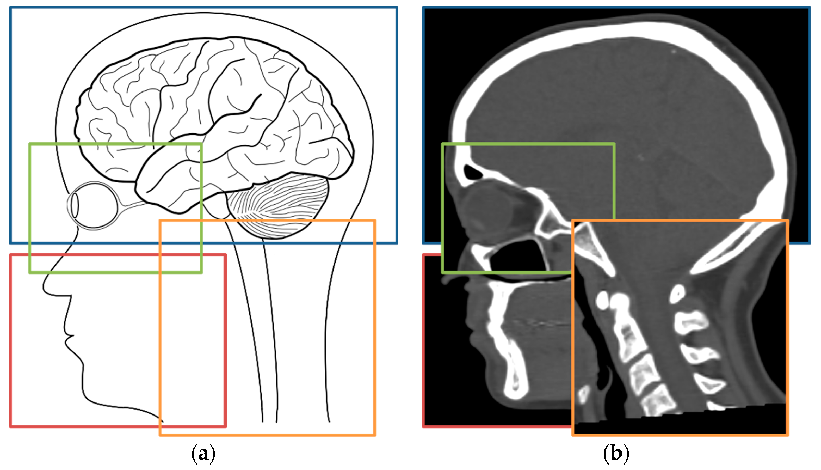
Figure 1. Head and neck whole field of views (FOVs) could be generated from joining several smaller parts from different patients as shown in the anatomical drawing in (a). Thus, overlapping incomplete CT scans such as a brain (blue box), facial orbits (green box), maxillofacial (red box), and neck (orange box), as shown in (b), could be equivalent to having a single scan covering the same FOV regarding pseudo-computerized tomography (pseudo-CT) synthesis pipelines.
Applsci 11 03508 g001
Figure 2. Representative magnetic resonance (MR)-CT pairs from the training dataset showing (ac) full head and neck MRs and (df) their corresponding paranasal sinuses, facial orbits, and brain CT images, respectively.
Applsci 11 03508 g002aApplsci 11 03508 g002b
Figure 3. Representative MR-CT pairs from the validation dataset showing (ac) full head and neck MRs and (df) their corresponding full head and neck CT images.
Applsci 11 03508 g003
Figure 4. Schematic representation of the Franken-net architecture. Our implementation in TensorFlow processes 3D cubes of the MR T1-weighted input image to generate a pseudo-CT cube with the same shape as the input.
Applsci 11 03508 g004
Figure 5. The residual block used in our architecture, it performs 2 convolutions and then the residual operation to avoid the degradation in the feature map generated.
Applsci 11 03508 g005
Figure 6. A schematic example of how the Atrous convolution operates depending on the dilation parameters, which determine the separation between the values selected by the kernel to perform the linear combination at each position.
Applsci 11 03508 g006
Figure 7. Loss function during training. The loss function used was the Mean Absolute Error (MAE) and the training was performed during 25 epochs (~500 k iterations).
Applsci 11 03508 g007
Figure 8. Examples of how the pseudo-CT synthetized by the network changes over the training process.
Applsci 11 03508 g008
Figure 9. Axial, Coronal, and Sagittal CT images from Subject fct-test-02 showed in (ac), respectively, and their corresponding computed pseudo-CT showed in (df). Bone delineation purpose looks quite good except for the neck region.
Applsci 11 03508 g009aApplsci 11 03508 g009b
Figure 10. Voxel-by-voxel correlation plot between CT and pseudo-CT of each dataset evaluation image, expressed in Hounsfield Units (HU) (a) and Bland–Altman plot between CT and pseudo-CT for all validation subjects (b). Gray scale bars show density of voxels in histogram grid. Axis representation is focused on values in the range of human tissues, from lungs to cortical bone.
Applsci 11 03508 g010
Table 1. Demographic and technical details from patients included in the training dataset.
Participant IDSexAgeField of View (FOV)
fct-train-01F31neck
fct-train-02F52paranasal sinuses
fct-train-03F74brain
fct-train-04F30neck
fct-train-05M34facial orbits
fct-train-06M25brain
fct-train-07M64brain
fct-train-08F66brain
fct-train-09F77brain
fct-train-10F65brain
fct-train-11M66brain
fct-train-12M80neck
fct-train-13M71neck
fct-train-14F63brain
fct-train-15F70facial orbits
Table 2. Demographic and technical details from patients included in the validation dataset.
Participant IDSexAgeFOV
fct-test-01M21full head
fct-test-02F46full head
fct-test-03M83full head
fct-test-04F38full head
fct-test-05F22full head
fct-test-06F27full head
Publisher’s Note: MDPI stays neutral with regard to jurisdictional claims in published maps and institutional affiliations.