Neural Networks—Deflection Prediction of Continuous Beams with GFRP Reinforcement

Abstract

Deflections on continuous beams with glass fiber-reinforced polymer (GFRP) reinforcement are calculated in accordance with the appropriate standards (ACI 440.1R-15, CSA S806-12). However, experimental research provides results which differ from the values calculated pursuant to the standards, particularly when it comes to continuous beams. Machine learning methods can be applied for predicting a deflection level on continuous beams with GFRP (glass fiber-reinforced polymer) reinforcement and loaded with a concentrated load. This paper presents research on using artificial neural networks for deflection estimation and an optimal prediction model choice. It was necessary to first develop a database, in order to train the neural network. The database was formed based on the results of the experimental research on continuous beams with GFRP reinforcement. Using the best trained neural network model, high accuracy was obtained in estimating deflection, expressed over the mean absolute percentage error, 9.0%. This result indicates a high level of reliability in the prediction of deflection with the help of artificial neural networks.

1. Introduction

The most commonly used material for reinforcing reinforced concrete (RC) elements in the construction of building structures is steel. Steel reinforcement is subject to corrosion that causes damage to the concrete and ultimately endangers the functionality and usability of reinforced concrete structures. Stopping the corrosion process is quite difficult and, often, without a significant effect. In addition, corrosion prevention costs can be significant. This fact is particularly important in reinforced concrete structures that are exposed to the aggressive action of the environment (marine structures, reservoirs, culverts, garages, etc.). This is the reason why fiber-reinforced polymer (FRP) reinforcement has been increasingly used instead of steel reinforcement.

FRP and steel reinforcement have different mechanical and deformation characteristics. FRP reinforcement, unlike steel reinforcement, has high tensile strength and a low modulus of elasticity. For these reasons, reinforced concrete elements made by using FRP reinforcement act differently compared to the elements with steel reinforcement.

As a consequence of the low elasticity modulus in RC elements, wider and deeper cracks appear, as well as larger deflections. Thus, in contrast with steel RC elements, the serviceability limit state of usability is very often relevant for design elements with FRP reinforcement. The behavior of simple beams with FRP reinforcement under operating load was the subject of experimental research. The results of these studies have yielded numerous formulas that have been proposed for determining deflection. Continuous beams reinforced with FRP reinforcement have also been the subject of experimental research, but to a much lesser extent. In general, experimental studies have obtained values which indicate that current regulations [1,2] underestimate the deflection values of continuous beams with glass fiber-reinforced polymer (GFRP) reinforcement under the action of load.

Some of the equations for calculating the deflection of continuous beams loaded with concentrated forces in the middle of the span are given in

Table 1. Some of the equations for calculating the deflection of continuous beams loaded with concentrated forces in the middle of the span.

Equation	Comment
$$\Delta =\frac{7}{768}\cdot \frac{P{L}^3}{E_c{I}_e}$$ (1)	Equation derived from elastic analysis
$${\Delta }_{\max }=\frac{P{L}^3}{48E_c{I}_{cr}}\left(\frac{5}{16}-\frac{15}{8}\left(1-\frac{I_{cr}}{I_g}\right)\cdot {\left(\frac{L_g}{L}\right)}^3\right)$$ (2)	The deflection calculation according to CSA S806-12 [2] is based on the moment–curve ratio along the span

.

In expression (1), $E_c{I}_e$ represents stiffness, and $I_e$ represents the effective moment of inertia of the observed cross-section. In Equation (2), $I_g$ represents the moment of inertia for the gross cross-section without fissures, and $I_{cr}$ represents the moment of inertia of a cracked cross-section.

Despite the existence of several equations for determining deflection, for continuous beams loaded with a concentrated load, it is not possible to determine this size absolutely precisely.

Deflection prediction for continuous beams can be performed by applying one of the artificial intelligence methods, artificial neural networks. This method is suitable for making predictions based on a large database. This paper presents its application. The database was formed from available data from, in this case, experimental research on continuous beams reinforced with GFRP reinforcement [3,4].

Application of Artificial Neural Networks in Construction

The beginnings of neural networks in construction date back to 1989, when the journal Microcomputers in Civil Engineering published a paper referring to the application of neural networks in this field. The authors of this paper are Adeli and Yeh [5]. The range of applications of artificial neural networks in construction is very wide. This method of artificial intelligence is used for the purpose of various types of predictions. The use of artificial neural networks in construction is becoming more common because of, in addition to the wide range of possibilities they have, the rapid development of software packages.

Predictions through the application of artificial neural networks are performed in all areas of construction. One of the predictions is the one about the cost of different construction structures, which was also addressed by a number of authors in their works [6,7,8,9,10,11,12]. In addition to prognostic costs, neural networks can also be used to predict the time required to complete construction projects, which has also been a topic addressed by some authors [13]. Predicting the quantity of material consumption for the construction of structures can, also, be conducting by applying neural networks. By applying neural networks, predictions of the behavior of structural elements in terms of boundary forces, deflections, fire resistance, etc., can also be made.

M. Knežević and R. Zejak developed a prediction model of experimental research for slim reinforced concrete posts with the help of neural networks (2008) [14]. The results of experimental research on 22 models of reinforced concrete slender columns were used to make the model. A prediction model for the limit force and maximum deflections in the directions of the main central axes of inertia in relation to the varied six input parameters was developed. This model showed satisfactory results, and its control resulted in an error smaller than 6% for the results prediction. It was proven in this way that neural networks can model nonlinear material behavior.

Artificial neural networks were also used to determine the fire resistance of reinforced concrete poles. The input data of this prediction model are: pole dimensions, concrete class, protective layer thickness, reinforcement percentage, load coefficient and aggregate type. The same data were calculated by the finite element method in combination with time integration using the FIRE program and neural networks. The obtained results, using both programs, for fire resistance are almost the same [15].

Dias and Pooliyadda defined a prediction model for predicting the strength of ready-mix concrete and high-strength concrete with chemical and mineral admixtures (Dias 2011) [16]. The authors used two types of neural networks (backpropagation and cascade correlation) (Alshihri 2009) to predict compressive strength for lightweight concrete mixtures of different ages. Prediction of the concrete admixture strength was conducted after three, seven, 14 and 28 days. The model has eight input variables: sand, water–cement ratio, lightweight aggregate, coarse aggregate, frozen smoke (aerogel) as an additive to cement, superplasticizer and a drying period. Compression force represents the output of the model. The research resulted in the conclusion that the model of cascade correlation gives more accurate results and learns very quickly compared to the backpropagation model [17].

Mohammadhassani and others, with the help of artificial neural networks, developed a prediction model for determining deflection in concrete beams. The defined model had 10 input values, two hidden layers and one output value. This model had high prediction accuracy and showed better results than the results obtained using linear regression. Model performance was measured via mean square error (MSE). The error value in the model of artificial neural networks is 40 times smaller than in the model of linear regression [18].

Hady presented the applications of neural networks in concrete structures. The author chose backpropagation networks which were written using the software MATLAB. It was concluded that NN are comparatively effective. Reasons for this conclusion lie in their ease of use and implementation and also NNs provide both the users and developers the possibility to cope with different kinds of problems [19].

Mohammed et al. used ANN with multilayer perceptron (MLP), utilizing a backpropagation (BP) algorithm, to foresee the shear quality of a reinforced concrete shaft [20].

A prognostic model for 28-day compressive strength was proposed by Hong et al. The authors used multilayer feed-forward NN for solving this problem. This model was defined to implement the complex nonlinear relation between the inputs and the output. Inputs were many factors that influence concrete strength, and the output was concrete strength. The neural network models provided high prediction accuracy and showed that usage of ANN for prediction of concrete strength is practical and beneficial [21].

Andres et al. explored application of ANN to predict the confined compressive strength and corresponding strain of circular concrete columns. Inputs of ANN consisted of the unconfined compressive strength, core diameter, column height, yield strength of lateral reinforcement, volumetric ratio of lateral reinforcement, tie spacing and longitudinal steel ratio. Outputs of ANN were confined compressive strength and the corresponding strain of circular concrete columns. The ANN model was compared to some analytical models and was found to perform well [22].

Mohammadi et al. used ANN for predicting the compressive strength of normal concrete and high-performance concrete. They concluded in their paper that a reliable model for predicting the compressive strength of concrete can save in time, energy and cost. That kind of model can also provide information about scheduling for construction and framework removal [23].

Mansoura et al. used ANN to predict the ultimate shear strengths of reinforced concrete (RC) beams with transverse reinforcements. The authors used test data of 176 RC beams. The data were arranged in the format of nine inputs (cylinder concrete compressive strength, yield strength of the longitudinal and transverse reinforcing bars, the shear span-to-effective depth ratio, the span-to-effective depth ratio, the beam’s cross-sectional dimensions and the longitudinal and transverse reinforcement ratios). The output of model was ultimate shear stress. The results show that ANNs have strong potential as a feasible tool for predicting the ultimate shear strength of RC beams with transverse reinforcement within the range of input parameters considered [24].

Naser et al. developed a model for predicting the fire resistance of reinforced concrete (RC) beams using ANNs. Beams were strengthened with carbon fiber-reinforced polymer (CFRP) plates, insulated with different protecting materials and exposed to different fire scenarios. Different insulation thicknesses, materials types and fire curves were the input parameters in the ANN model and fire endurance and time to failure were the output parameters. The predicted values were compared with experimental values and validated finite element study results, and strong correlations between those were obtained [25].

Mangalathu et al. introduced application of machine learning techniques to identify the response mechanism, including the classification of the failure mode and the prediction of the associated shear strength of beam–column joints. The authors used 536 experimental data to develop a model. The model can be used by engineers to design new structures and also for the assessment and repair strategy of existing buildings [26].

2. Materials and Methods

In this paper, we used the data obtained in an experimental research which was conducted on two-span continuous beams with GFRP reinforcement and loaded with concentrated forces in the midpoints of the spans.

After data collection, their analysis was performed. The next step was to prepare the analyzed data for model formation. The last step was to define the final model for the prediction of deflections in continuous beams.

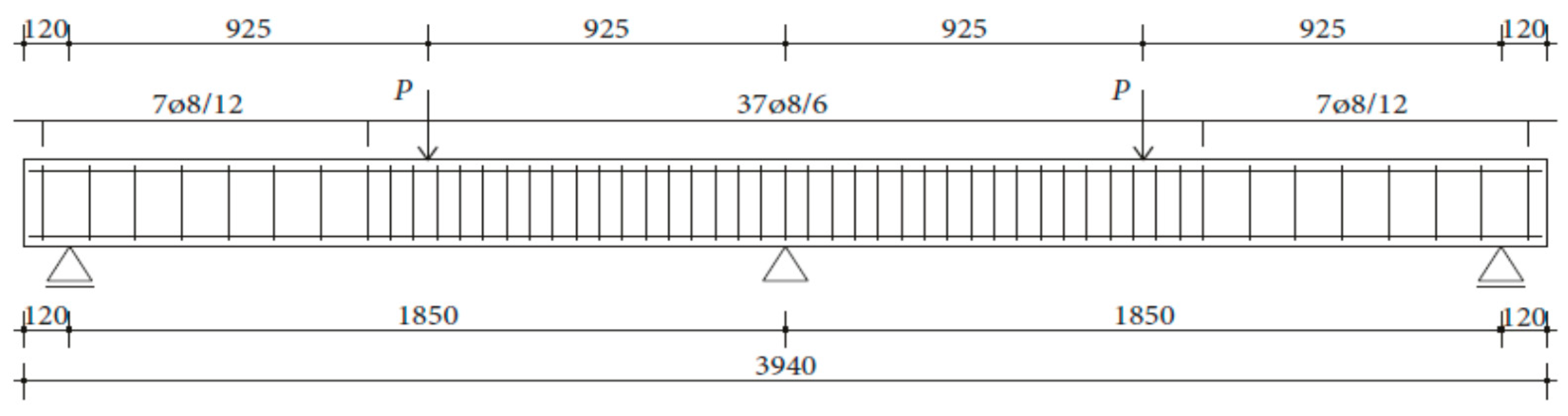
The experimental research included 11 continuous beams with a total length of 394 cm. The beams were on two spans 185 cm long and with overhangs of 12 cm each (see Figure 1).

The cross-sectional dimensions of the beams were 15 × 25 cm. Details of all 11 experimental beams are given in

Table 2. Details of experimental beams.

Beam	Longitudinal Reinforcement Support—Upper Zone	Longitudinal Reinforcement Midspan—Lower Zone	Reinforcement	Cross-Section
B1	3Φ14	2Φ12 + 1Φ10	GFRP polyester—wrapped
B2	2Φ10 + 1Φ14	2Φ12 + 1Φ14	GFRP polyester—wrapped
B3	2Φ10 + 1Φ12	2Φ14 + 1Φ12	GFRP polyester—wrapped
B4	3Φ12	3Φ10	GFRP polyester—wrapped
B5	2Φ9 + 1Φ12	2Φ12 + 1Φ9	GFRP polyester—wrapped
B6	2Φ9 + 1Φ10	2Φ12 + 1Φ10	GFRP polyester—wrapped
B7	3Φ7	2Φ6 + 1Φ7	GFRP polyester—wrapped
B8	2Φ6 + 1Φ7	2Φ7 + 1Φ6	GFRP polyester—wrapped
B9	4Φ12	2Φ10 + 2Φ9	GFRP epoxy—ribbed (deformed)
B10	3Φ10 + 1Φ12	2Φ12 + 2Φ9	GFRP epoxy—ribbed (deformed)
B11	3Φ9	3Φ12 + 1Φ10	GFRP epoxy—ribbed (deformed)

.

The beams were loaded with concentrated loads in the midpoints of both spans up to failure. Nine beams were reinforced with GFRP longitudinal and transverse reinforcement to experience concrete compression failure, while two beams were designed to experience FRP reinforcement failure. The main parameters which vary are the ratio of quantities of longitudinal reinforcement in the middle of the span and above the support—in other words, the designed redistribution of moments—the percentage of reinforcement with longitudinal reinforcement and the type of GFRP reinforcement.

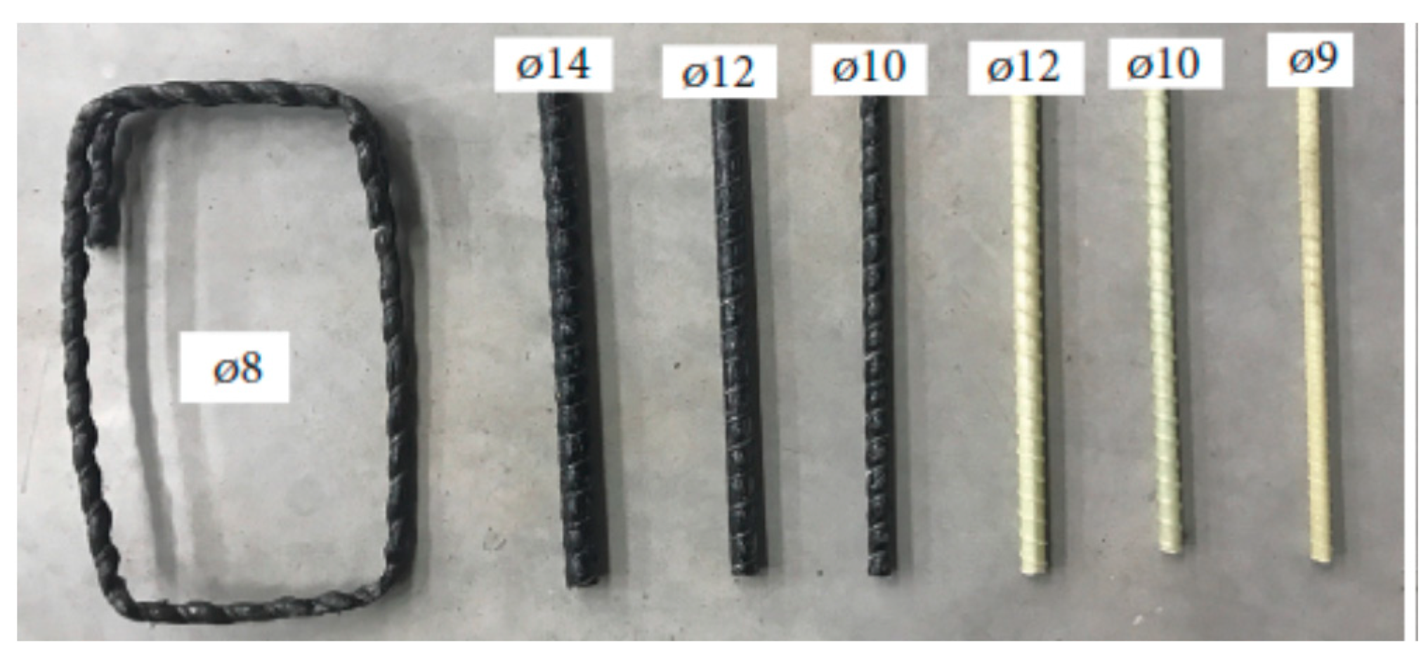
Two types of GFRP bars were used for the longitudinal reinforcement: GFRP reinforcement with 70% longitudinal fiberglass (E-glass) in total volume, impregnated in an unsaturated polyester matrix, and GFRP reinforcement with 75% longitudinal fiberglass (E-glass), impregnated in an epoxy matrix. GFRP reinforcement with polyester was wrapped in fiberglass, while GFRP reinforcement with epoxy was ribbed (Figure 2), in order to improve the adhesion conditions between the concrete and reinforcement. GFRP stirrups with polyester were used in all the beams.

Two designed concrete classes were used in the experiment of 28 MPa and 40 MPa, which represent compressive strength concrete cylinders with the dimensions 15/30 cm.

Continuous beams were placed on three supports over steel bearings. The end supports were designed to be movable in the horizontal direction. The middle support was designed so that horizontal movement is prevented. The load was applied with the help of hydraulic presses placed in the middle of both spans (Figure 3).

Deflections along the spans of continuous beams were measured with electric LVDT transducers, the accuracy of which was 1/100 mm (in the middle of the span) and 1/50 mm (in quarters of the span). They were placed on the lower edge of beams in quarters of the span, i.e., there were three LVDT transducers in each span.

This was a load-controlled experiment. A monotonically increasing static load was gradually applied at the beams in increments from zero to failure. The load was applied in increments from 2 to 5 kN at the very beginning, and then, after cracks started appearing, in increments of 5–10 kN. Results were measured on each 5 kN. The loading rate was about 5 kN/min.

The measurement was performed after each load increment. The effective moment of inertia changes for each step as the load is applied. The highest value is the gross concrete cross-section. The effective moment of inertia decreases with increasing load and is calculated by formula (3) [3]:

$$I_e={\left(\frac{M_{cr}}{M_a}\right)}^3·{\beta }_d·I_g+\left(1-{\left(\frac{M_{cr}}{M_a}\right)}^3-K\right)·I_{cr}·0.7\le I_g$$

(3)

where K is calculated by formula (4) [3]:

$$K={\left(\frac{1}{11}·\left(\frac{M_{cr}}{M_a}\right)\right)}^4$$

(4)

This is a proposed formula for the effective moment of inertia based on experimental results for six beams [3]. $M_{cr}$ is a moment at the appearance of the first crack (cracking moment). The force at the appearance of the first crack is defined, as well as the moment $M_{cr}$, on the basis of the measured reactions at the ends of the beam and the force itself. $M_a$ is a moment corresponding to each load increment. It changes with the change in force both in the midspan and above the support.

For the purposes of forming the prediction model, data were selected and collected, and the values of the force applied in the midpoints of the beam span, the value of the effective moments of inertia of the cross-section in the middle of the span and above the support and the deflection values were measured.

After the data were collected, determining the input model data was performed. The criterion for their choice was their direct impact on deflections. Based on the previous, the input variables were selected, namely: force, effective moment of inertia of the cross-section in the middle of the span and effective moment of inertia of the cross-section above the support. In addition to the above values, the deflection is affected by the span and cross-section. In the conducted experiment, these quantities were identical so that they were not chosen for the input variables of the model. The percentage of reinforcement was considered through the effective moments of cross-section inertia. Data were collected from the conducted experimental research. The input data, with their limit and mean values, are shown in

Table 3. Input data.

Input Data Number	Input Data Description	Data Type	Units of Measure	Min	Max	Mean Value
Input 1	Force	numerical	kN	5	137.75	55.571
Input 2	Effective moment of inertia of the cross-section in the middle of the span	numerical	mm4	328.0033	19,531.25	2011.399
Input 3	Effective moment of inertia of the cross-section above the support	numerical	mm4	290.1866	19,531.25	1965.198

.

The next step was to define the output from the model. Based on the considered parts of the research, it was determined that the model has one output which is a deflection in the midpoint of the continuous GFRP-reinforced beam (see

Table 4. Output data of the model.

Output Data Number	Output Data Description	Data Type	Units of Measure	Min	Max	Mean Value
Output 1	Deflection	numerical	mm	0.11	31.20	9.703	$\left(-\infty ,+\infty \right)$

).

There are various recommendations in the literature for dividing available data into training and test sets. The authors generally selected data at 90% to 10%, 80% to 20% or 70% to 30% [27]. In addition to the established practice in choosing the percentage of each of the sets, the specificity of each of the problems to be solved determines the appropriate relationship between these two sets. In this research, a division of 80–20% of the training set in relation to the test set was adopted. In eight models, a direct division into training and test sets was performed, and in 2 models, random data selection was conducted. The cross-validation procedure (kFold-CrossValidation and LeaveOneOut-CrossValidation) performed the random data selection.

The dataset was formed using data from experimental research. The total number of datasets was 355. Each dataset was obtained after each increase in load, i.e., about 30 records for each beam. From this total number of sets, 284 datasets were determined to form a training set, whereas the remaining 71 datasets formed a test set. This division was in the ratio of 80% to 20% for training and test.

Before starting the network training, it was necessary to process the data, i.e., to perform their scaling so that they all fall within a certain range of sizes. Some of the methods for data scaling are standardization and normalization [28,29]. The result of these methods is the reduction of certain data to the same order of magnitude. Additionally, they provide an opportunity to perform data analysis with the same significance during the formation of the model, which means that they will provide data analysis with a smaller size range [29]. Min-max normalization methods for data scaling and StandardScalar (Z-score normalization) were used in this study.

The first step in forming a network is to determine the architecture of the network. Determining the network architecture is defining the number of layers and the number of neurons in each of the layers. Recommendations can be found in the literature, but not unambiguously defined formulas that result in the number of layers in the network as well as the number of neurons in the layers. Networks with two hidden layers have given reliable results in numerous simulations in various engineering fields. Nevertheless, the number of layers needs to be adjusted to the specifics of the problem being solved. This is the reason why in the literature we often find good prediction results and the use of neural networks with three or more hidden layers.

An unadjusted number of neurons leads to overfitting or underfitting. The problem of overfitting appears in case of a large number of neurons, whereas the unsatisfactory number of neurons leads to the problem of underfitting, i.e., of the dependence between input and output quantities. The number of neurons should be such so as to enable the data to show their most useful characteristics and not cause any of the stated issues.

The number of layers and the number of neurons in each of the layers was, in this study, determined experimentally.

The aim of the model-defining process is finding a model with the best possible generalization capacity. Generalization is a process in which the knowledge that is valid for a set of cases is transferred to a superset of it [30], i.e., the model has the ability to result in satisfactory sizes based on data that were not presented to it during training. The possibility of improving the generalization in the prediction is provided by the use of the cross-validation procedure.

In the process of finding the most reliable model, the prediction error is constantly calculated. The prediction error is the difference between the actual (desired) and the predicted value and it defines the model accuracy measure. There are a number of predictive accuracy measures in the literature. For the purpose of defining the prognostic model in this research, the mean absolute percentage error (MAPE) was taken as a measure of accuracy. Expression (5) shows the mean absolute percentage error, where Ai is the expected value, and Fi is the predicted value.

$$\mathrm{MAPE}=\frac{1}{N}{\displaystyle \sum }_{i=1}^n\left|\frac{A_i-F_i}{A_i}\right|$$

(5)

The prediction model was formed in the Python 3.7.6 software package. To solve the problem that is the subject of the research, a multilayer perceptron (MLP) was formed, which is one of the types of artificial neural networks.

The activation functions of neurons in the hidden layers that are most commonly used are logistic sigmoid (logistic), hyperbolic tangent (tanh) and rectified linear unit function (ReLu). In addition to the above, in the field of artificial neural networks, the authors began to use a new activation function of hidden layers called Swish. Output neurons generally have a linear activation function. Given the nature and characteristics of the data, the corrected linear unit (ReLu) function, the hyperbolic tangent (tanh) and the Swish function were used in this research to define the model, and the Identity function was used for the output neurons (see

Table 5. Activation functions of a multilayer perceptron model of an artificial neural network.

Function	Mark	Explanation	Range
Identity	$x$.	ly in the output layer	$\left(-\infty ,+\infty \right)$
Rectified Linear units	$max\left(0,x\right)$	Activation of neurons is transmitted directly as an output if it is positive, and if it is negative, 0 is transmitted. It has been proven to have 6 times better convergence compared to the hyperbolic tangent function.	$\left(0,+\infty \right)$
Hyperbolic tangent	$\frac{2}{\left(1+e^{-2x}\right)}-1$	Activation of neurons is transmitted directly as an output if it is positive, and if it is negative, 0 is transmitted.	$\left(-1,1\right)$
Swish	$x\ast sigmoid\left(x\right)$	A function that is nonlinearly interpolated between a linear and a ReLu function.	$\left(0,x\right)$

).

3. Results and Discussion

Based on the defined input and output variables and other necessary parameters, models of artificial neural networks—multilayer perceptron (MLP)—were defined. The number of layers, as well as the number of neurons in hidden layers, is determined experimentally, and the number of neurons in the input and output layer is determined based on the number of input and output values. The number of hidden layers was increased from one to three during the model formation. The largest number of hidden neurons in each of the hidden layers is 15. Ten models of artificial neural networks were formed. In five models, the data were scaled using the min-max procedure, while in the remaining five models, the StandardScalar procedure was used.

All neural networks in the model have three input values and one output value. Models of neural networks with min-max standardization for predicting the deflection of continuous beams are shown in the following table (see

Table 6. Models of artificial neural networks for continuous beam deflection estimate (min-max).

Model Name	Model Characteristics	Activation Function of Hidden Layers	Activation Function of Output Layer	MAPE Training Set [%]	MAPE Test Set [%]
NND4	MLP 3-7-14-3-1	ReLu	Identity	9.89	13.40
NND5	MLP 3-7-13-3-1	Tanh	Identity	13.82	13.55
NND6	MLP 3-7-9-3-1	Swish	Identity	13.48	13.45
NND8	MLP 6-7-7-3-1	ReLu	Identity	11.75	12.61

). It also lists the characteristics of each model with a measure of accuracy determined by means of the mean absolute percentage error (MAPE).

Models of neural networks formed with data scaled using the StandardScalar normalization procedure are shown in the following table (see

Table 7. Models of artificial neural networks for continuous beam deflection estimate (StandardScalar).

Model Name	Model Characteristics	Activation Function of Hidden Layers	Activation Function of Output Layer	MAPE Training Set [%]	MAPE Test Set [%]
NND1	MLP 3-7-15-3-1	ReLu	Identity	10.62	21.34
NND2	MLP 3-7-12-3-1	Tanh	Identity	14.61	11.83
NND3	MLP 3-7-15-3-1	Swish	Identity	8.56	9.00
NND7	MLP 3-7-8-3-1	ReLu	Identity	8.97	17.84

). This table also shows the characteristics of the models as well as the accuracy of the estimate obtained by the mean absolute percentage error (MAPE).

In two models, random data selection was performed. In one model, it was conducted using kFold-CrossValidation for k = 10 and in the other one using LeaveOneOut-CrossValidation (LOOCV). The accuracy measure of these models is determined using the mean absolute percentage error (MAPE) (see

Table 8. Models of artificial neural networks with random choice of data for continuous beam deflection estimate (kFold-CrossValidation, k = 10).

Model Name	Data Scaling Procedure	Model Characteristics	Activation Function of Hidden Layers	Activation Function of Output Layer	MAPE [%]	σ [%]
NND9	StandardScalar	MLP 3-7-13-3-1	ReLu	Identity	33.61	15.22

and

Table 9. Models of artificial neural networks with random choice of data for continuous beam deflection estimate (LOOCV).

Model Name	Data Scaling Procedure	Model Characteristics	Activation Function of Hidden Layers	Activation Function of Output Layer	MAPE Training Set [%]	MAPE Test Set [%]
NND10	Min-Max	MLP 3-7-14-3-1	ReLu	Identity	11.05	13.50

). In models where dividing data was conducted by using kFold-CrossValidation, the data were scaled with StandardScalar, and in those models in which the division was performed using LOOCV, the data were scaled through the min-max function. The two models that gave the best results in each of the random data selections are presented here.

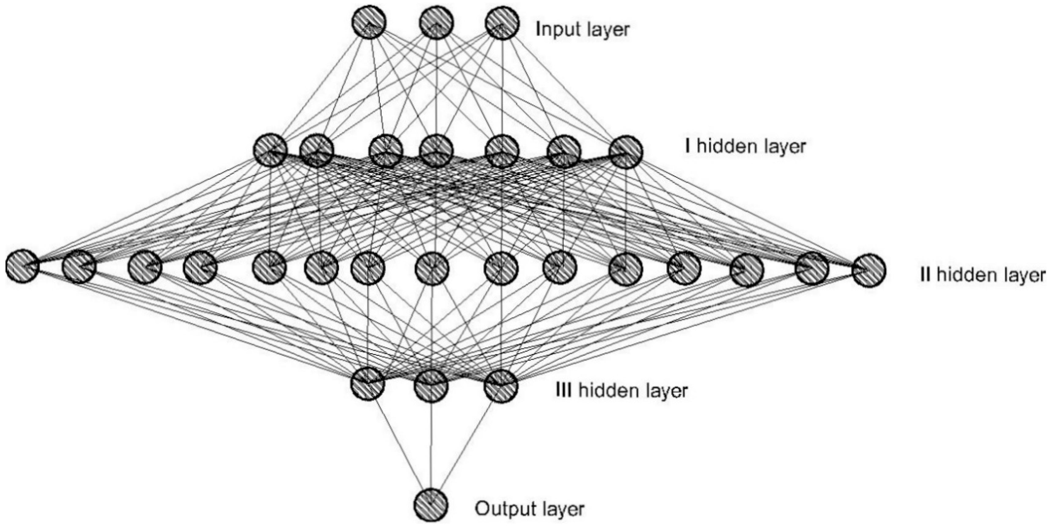
Considering and comparing the presented models, it is noticed that the NND3 model has the best performances, i.e., gives the smallest error in the prediction. For the NND3 model, data scaling was applied using StandardScaler. It defines one input, three hidden and one output layer of neurons. There are three neurons in the input layer. In the hidden layers, from the first to the third, there are seven, 15 and three neurons. There is one neuron in the output layer. The architecture of the neural network is shown in Figure 4. The activation function of the hidden layer is the function of the rectified linear unit (Swish). The number of conducted epochs of the model with the highest accuracy is 1000. The measure of the accuracy of model estimation is expressed through the mean absolute percentage error and amounts to 9.00%.

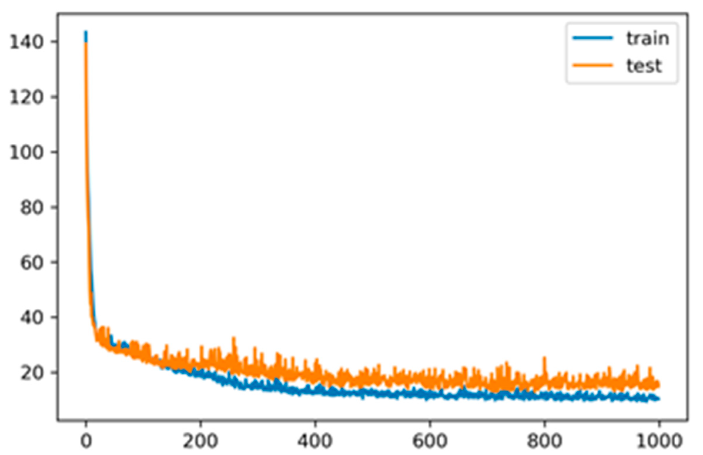
The following diagram shows the value of the mean absolute percentage error per training and test set, depending on the number of epochs when training the artificial neural network (see Figure 5).

The relationship between the values obtained in the experimental study and the predicted values with the help of neural networks on the training and test sets is shown in the following diagram (see Figure 6). Deflection values obtained by prediction on training and test sets converge to the line, and this indicates the high reliability of the prediction.

The model with the highest accuracy is the model on the basis of which the final model for estimating the deflection of continuous beams reinforced with GFRP reinforcement was made and on the basis of which the prediction model was defined.

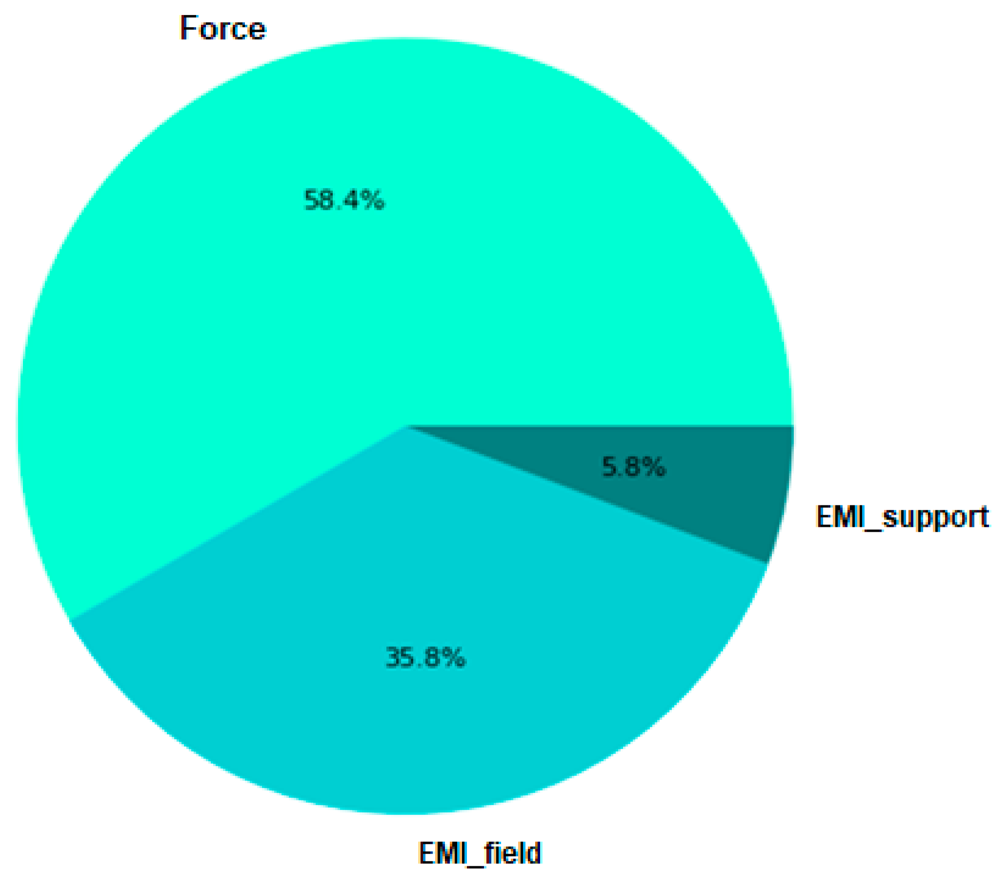
The sensitivity of the output value on the input variables, i.e., the influence of the force, effective moment of inertia of the cross-section in the middle of the span (EMI_field) and effective moment of inertia of the cross-section above the support (EMI_support) on the value of deflection, is shown in the following diagram (Figure 7). The diagram clearly shows that the force has the greatest influence on the value of deflection, 58.40% in relation to the effective moments in the middle of the span and above the support.

4. Conclusions

This paper presented the application of artificial neural networks with the purpose of estimating deflection values on continuous beams with GFRP reinforcement by applying the concentrated force in the midpoints of the spans.

Based on the results presented in the research, it is concluded that the model with the highest accuracy of deflection estimation in continuous beams with GFRP reinforcement and loaded with concentrated force in the midpoints of the spans is a model of an artificial neural network whose architecture is presented with one input, three hidden layers and one output layer of neurons. There are three neurons in the input layer of neurons, seven neurons in the first hidden layer of neurons, 15 in the second and three in the third and one neuron in the output layer of neurons. The activation function of the hidden layers of neurons is Swish, while the activation function of the output layer is linear (Identity). The number of epochs conducted on the model is 1000. The measure of model accuracy is represented by the mean absolute error (MAPE). Its value for models with the best performance is MAPE = 9.00%.

The accuracy of the prediction model can be improved by increasing the number of data in the database. In addition to this, the prediction model would have the possibility of wider application if the database were expanded with certain material characteristics or continuous beam characteristics. Some of the characteristics could be: cross-section of a beam, type of FRP reinforcement, the percentage of reinforcement in the span, the percentage of reinforcement above the support, ratio of percentage of reinforcement in the span and above the support, etc. Potential parameters which could be used for expanding the database would, actually, be the input parameters of the prediction model.

The high reliability of the prediction model confirms the possibility of using artificial neural networks for the purpose of deflection prediction. This statement is important in the fact that the deflection calculation by using conventional computing techniques is quite complex. The advantage of neural networks is that they can solve new problems, based on previously learned solved problems. In addition to this, they have an advantage which is reflected in their adaptability. The reliability of prediction models made by neural networks depends on the quality and quantity of data. Experimental research provides a large amount of high-quality data. The data used to define the prediction model for deflection prediction are those from an experimental study conducted on eleven continuous beams with GFRP reinforcement. The beams were loaded with concentrated forces in the midpoints of the spans and the deflection was measured in the midpoints of the spans.

Based on all of the above, it can be concluded that neural networks represent a reliable method for deflection estimation on GFRP-reinforced continuous beams under load with concentrated forces in the midpoints of the spans.