1. Introduction
The process of odor perception is more complicated than visual and auditory perception [
1]. It is the result of the aggregate activations of 300 to 400 different types of olfactory receptors (ORs) [
2], expressed in millions of olfactory sensory neurons (OSNs) [
3,
4]. These OSNs send signals to the olfactory bulb, then further to structures in the brain [
5,
6]. The olfactory signals are ultimately transformed into verbal descriptors, such as “musky” and “sweet”.
Compared with visual and auditory perception, odor perception is quite difficult to describe. The odor impression of human beings is affected by culture background [
7], gender [
8], and aging [
9]. There are variabilities between people in the evaluation of odor perception. Besides, the relationships between odorants and odor perception remain elusive. Although some work has revealed some physicochemical features of the odorants, such as the carbon chain length [
10] and molecular size [
11], are related to human odor perception, the odorant molecules with similar structures could smell quite different. In contrast, the molecules with distinct structures could be described in an identical way [
12]. In summary, odor perception is an exciting but challenging issue in the field of odor research.
Currently, semantic methods are the most widely used approaches to qualify odor perceptions in practice [
13,
14,
15]. Each odor perception descriptor corresponds to one odor perception, so they are considered equal in this paper.
Semantic odor perception descriptors have played an important role in food [
16,
17], beverage [
18,
19], and fragrance engineering [
20] for product quality assessment and other commercial environments [
21]. Therefore, numerous domain-specific sets of verbal descriptors for qualifying odor perception have been derived [
19,
22,
23,
24]. Croijmans et al. revealed a list of 146 wine-specific terms used in wine reviews [
19]. The American Society for Testing and Materials (ASTM) Sensory Evaluation Committee reviewed literature and industrial sources and collected over 830 odor descriptors in use. Different from the traditional manual design approaches, Thomas et al. developed a standardized odor vocabulary in an automatic way [
25]. They proposed a data-driven approach that could identify odor descriptors in English and used a distributed semantic word embedding model to derive its semantic organization. In summary, the odor vocabulary is a colossal family, which increases the difficulty of odor sensory assessment in the industries. The previous odor perception works have focused on deriving more and more verbal descriptors relating to odor perception, leading to redundancy in these odor perception descriptors. The identification of the redundant odor perception descriptors is a “blank” area. In the paper, we aim to fill this gap.
Using these odor perception vocabularies, a lot of odorant-psychophysical datasets were developed [
26,
27,
28]. The well-known Dravnieks dataset [
29] contains 144 mono-molecular odorants, and their expert-labeled perceptual ratings of 146 odor descriptors range from 0 to 5. The DREAM dataset [
30] involves 476 molecules and their perceptual ratings of 21 odor perception descriptors labeled by 49 untrained panelists, ranging from 0 to 100. These psychological odor datasets contain exuberant information on the relations between different odor perceptions. Base on these odorant-psychophysical datasets, Substantial efforts have focused on the odor perception space and the relations among different odor perceptions.
There are two main viewpoints on the dimensions of the odor perception space: low dimension and high dimension. For the low dimension viewpoint, Khan et al. found that pleasantness was the primary dimension of the odor perceptual space by principal component analysis (PCA) [
31], and this finding was validated by a series of studies [
32,
33,
34]. However, the degree of pleasantness is too coarse to describe the details of odor perception. Jellinek developed an olfactory representation referred to as odor effects diagram with two fundamental polarities: erogenous versus antierogenous (refreshing) and narcotic versus stimulating [
35]. Zarzo and Stanton obtained similar results to the odor effects diagram by applying PCA to two public databases [
20]. For the high dimension viewpoint, Mamlouk and Martinetz reported that an upper bound of 68 dimensions and a lower bound of at least 32 Euclidean dimensions for the odor space was revealed by applying multidimensional scaling (MDS) on a
dissimilarity matrix derived from Chee-Ruiter data originated from Aldrich Chemical Company’s catalog [
36]. Tran et al. implemented the Isomap algorithm to reduce the dimensions of human odor perceptions for predicting odor perceptions [
37]. Castro et al. identified ten primary dimension axes of the odor perception space by using non-negative matrix factorization (NMF), in which each axis was a meta-descriptor consisting of a linear combination of a handful of the elementary descriptors [
38]. In short, there is no consistency in the structure of the odor perception space. Moreover, all of these works are based on the transformation approaches, and each dimension comprises multiple-element odor perceptions. Different from that, We propose a selection mechanism to narrow down the numbers of odor perception descriptors. Based on this selection mechanism, every odor perception descriptors’ meaning remains, whose meaning is easily understood. Hence, the odor experts only need to rate much fewer odor perception descriptors so that the odor assessment workload is alleviated dramatically.
For the relations between different odor perceptions, due to the linguistic nature of odor perception descriptors, natural language processing (NLP)-based approaches have been introduced [
25,
39,
40,
41,
42]. Debnath and Nakamoto implemented a hierarchical clustering based on the cosine similarity matrix, which was calculated from the 300-dimensional word vectors of 38 odor descriptors [
43]. However, it mainly focuses on the prediction of odor perceptions. The reduced outputs are more intangible and harsher than the originals, and the details of the original perception information were lost. Li et al. investigated the internal relationship between the 21 odor perceptual descriptors of the DREAM dataset and found that pleasantness was inferred from “sweet” precisely, which implied that some of the odor perceptions overlapped with others. Nonetheless, 21 descriptors are insufficient to describe the entire odor perception [
44]. In summary, the relationship between these odor perceptions has not been thoroughly investigated.
To address the issues of reducing the odor vocabulary, inspired by the conception of primary odorants [
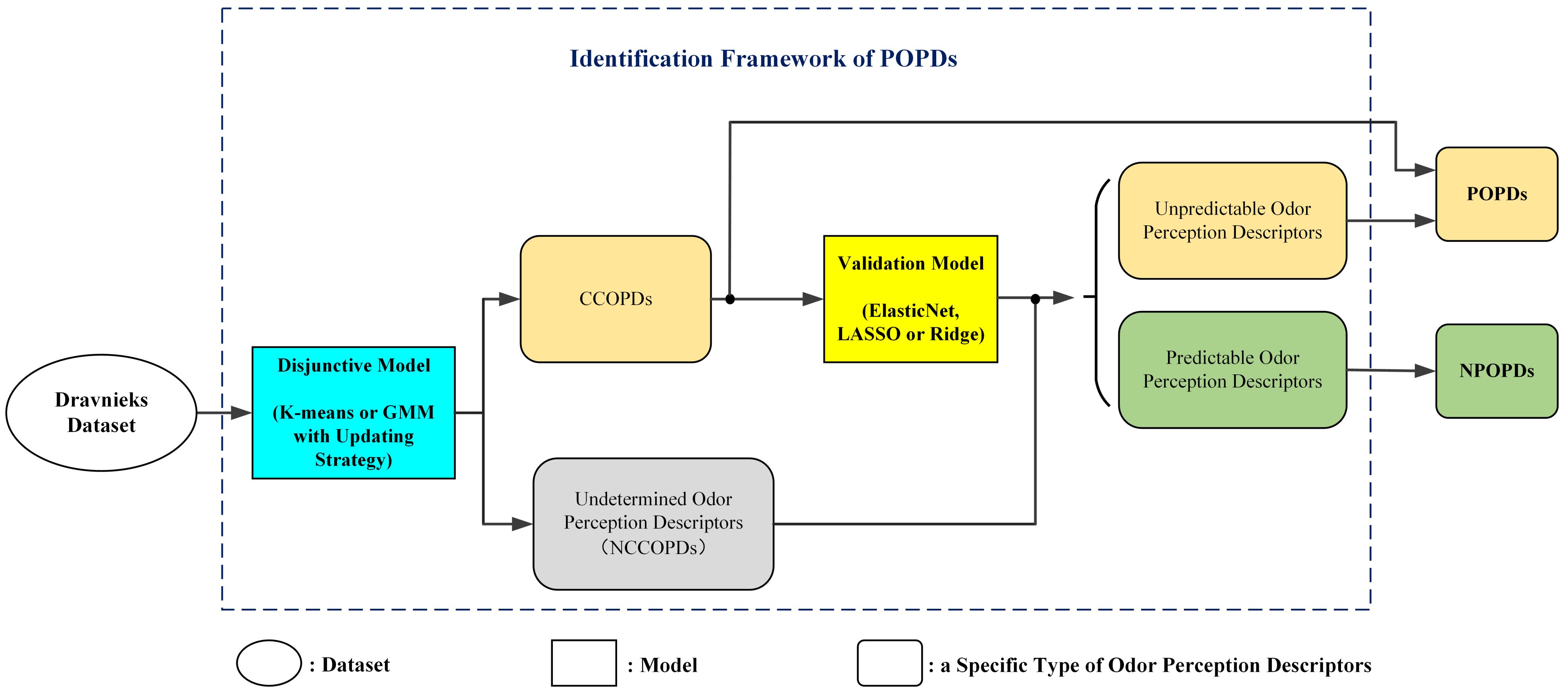
45], the chemicals which the specific anosmias are mapped, we proposed the definition of primary odor perceptual descriptors (POPDs), defining as the smallest set of odor perception descriptors. The perceptual ratings of the other odor perception descriptors, namely non-primary odor perception descriptors (NPOPDs), could be inferred or predicted precisely from those of the POPDs. It should be noted that the POPDs only relate to human odor perception and have no relation with the odorants. To identify the POPDs and NPOPDs, we proposed a novel selection mechanism based on machine learning, as described in
Figure 1.
The identification framework of POPDs comprises the disjunctive and validation models. The disjunctive model is employed to identify the Clustering-Center Odor Perception Descriptors (CCOPDs) and Non-Clustering-Center Odor Perception Descriptor (NCCOPDs). The CCOPDs are part of the POPDs. The NCCOPDs are also called undetermined odor perception descriptors, which may be POPDs or NPOPDs. The validation model is implemented to distinguish the POPDs and NPOPDs in NCCOPDs, whose inputs are the CCOPDs and the outputs are the NCCOPDs. If the perceptual ratings of the NCCOPDs could be predicted precisely by those of the CCOPDs, they are predictable and regarded as redundant. Therefore, they are identified as the NPOPDs. The NCCOPDs, which could not be predicted precisely, are unpredictable and identified as the POPDs together with the CCOPDs.
The identification framework proposed in this paper is essentially a selection strategy. No transformation is made on these odor perception descriptors, so the POPDs are a subset of all the odor perception descriptors, and their original meanings retain.
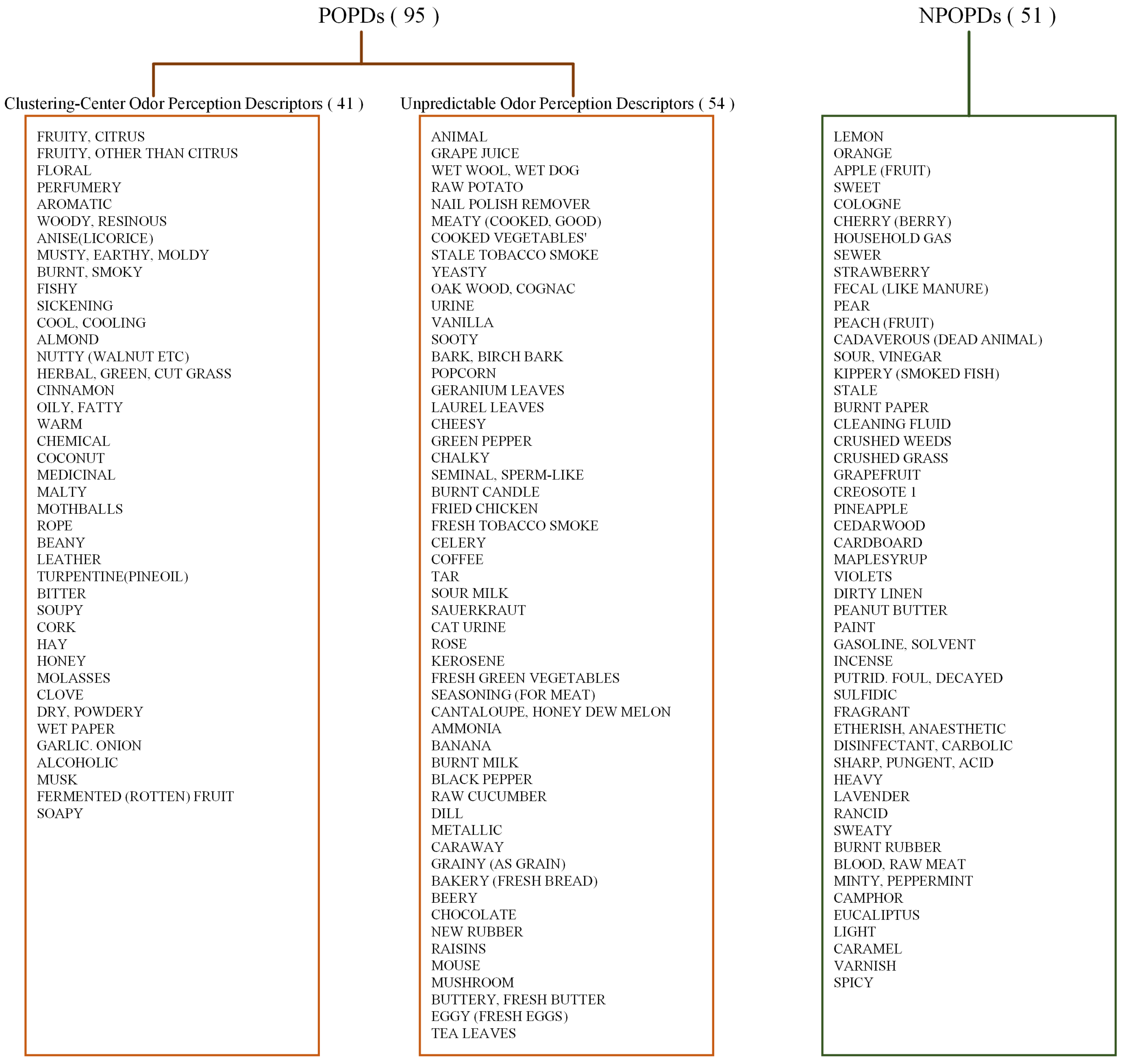
To summarize, all of the odor perception descriptors fall into two categories: POPDs and NPOPDs. Moreover, the POPDs include CCOPDs and unpredictable odor perception descriptors, as shown in
Figure 2. It should be noted that the NPOPDs are inferred from the CCOPDs only. Besides, the identification framework also reveals the complicated relations between these odor perceptions. The POPDs can be used as the axes to construct a quasi-odor perception space to describe human odor perception. Therefore, it will shed light on the research of odor perception space.
Specifically, the main contributions of this work are as follows.
- (1)
Unlike the current work focusing on developing more odor perception descriptors, we propose the task of narrowing down the number of the odor vocabulary and a novel definition of POPDs.
- (2)
Different from the transformation approaches, a selection mechanism based on machine learning is proposed to identify the POPDs and NPOPDs. It demonstrates that dozens of odor descriptors are redundant, which could be removed from the odor vocabulary. The relationship between POPDs and NPOPDs is revealed by the disjunctive model, which provides the mapping functions between the odor perception descriptors.
- (3)
The effects of the sparsity of odor perception data and the correlations between odor perceptions on the predicting model’s performance are investigated, respectively.
The remainder of this paper is organized as follows.
Section 2 presents the materials and methods. The experiment and results are discussed in
Section 3. The discussion is given in
Section 4. Finally,
Section 5 concludes this paper.
2. Materials and Methods
2.1. Data and Description
Compared with the other odor perceptual datasets, the structure of the Dravnieks psychophysical dataset is much denser [
46], which is beneficial for the identification of POPDs. Therefore, the Dravnieks dataset is adopted in this work. It contains 144 mono-molecule odorants and their corresponding perceptual ratings of 146 odor perception descriptors, forming a
matrix [
29]. Each column of this matrix is a 144-dimensional odor perception descriptor vector, representing the odor perception descriptors. Each row of this matrix is a 146-dimensional molecular vector, representing the odorants or molecules. These odor descriptors were selected by ASTM Sensory Evaluation Committee, which reviewed the literature and industrial standards for odor evaluation. A large evaluation team composed of 150 experts evaluated the perceptual ratings ranging from 0 to 5. Therefore, compared with other odor psychophysical datasets, these data have a high degree of consistency and stability. The Percent applicability (PA) scores of these odorants were used for POPDs identification [
13].
Considering that sparsity is a significant characteristic of odor psychophysical data, the sparsities of odor perception descriptors and molecules are calculated. The sparsity of each molecule is defined as:
where
is the count of perceptual ratings with a value of 0 in each 146-dimensional molecular vector.
is the total number of odor perception descriptors, with a value of 146.
The sparsity of each odor perception descriptor is given as follows:
where
is the count of elements with a value of 0 in each 144-dimensional odor perception descriptor vector, and
is the total number of odor molecules, with a value of 144.
The sparsity for the Dravnieks dataset is given as:
where
is the count of perceptual ratings taking the value of 0 in the
perceptual matrix, and
N is the total number of elements of the dataset, i.e.,
.
The
correlation matrix of odor perception descriptors is calculated. The Pearson correlation coefficient between every two 144-dimensional odor perception descriptor vectors is formulated as follows:
where
,
are the 144-dimensional odor perception descriptor vectors, and
,
are the means of
,
, respectively.
2.2. POPDs and the Identification Frameworks
As shown in
Figure 1, there are two parts in the identification framework: disjunctive model and validation model. The disjunctive model is employed to obtain the optimal inputs of the validation model, which are used to predict as many as possible NCCOPDs precisely. The validation model is conducted for the prediction of NCCOPDs, distinguishing the predictable and the unpredictable ones. The mapping functions between the CCOPDs and the NPOPDs are established.
Inspired by [
38,
41], the odor perceptions cluster in the odor perception space, and the clustering centers are the representatives of the clusters. Therefore, the clustering algorithms with an updating strategy are adopted as the disjunctive models. Considering that ball-shaped clusters’ clustering centers could represent the other points in the same cluster better than those of irregular-shaped clusters, the K-means algorithm and Gaussian mixture model (GMM) with an updating strategy for identifying CCOPDs are used as the disjunctive model. These two kinds of disjunctive models are called the K-means-disjunctive model and GMM-disjunctive model, respectively.
It should be noted that the CCOPDs obtained from the disjunctive models with an updating strategy are not the clustering centers determined only by the clustering algorithms. Therefore, the conclusion drawn from any clustering algorithm is no longer suitable for these CCOPDs. In other words, the disjunctive models’ results could not be explained by the clustering theory, and these results could not reveal the structure of odor perception space and any relationship between these odor perception descriptors. The disjunctive model is only used to identify some critical odor descriptors with a high probability.
To validate which NCCOPDs could be inferred or predicted precisely by the CCOPDs, three classical and stable linear regression models, namely Ridge regression, LASSO regression, and ElasticNet regression, are implemented as the validation model.
Consequently, there are six combinations for the identification frameworks: K-means-Ridge, K-means-LASSO, K-means-ElasticNet, GMM-Ridge, GMM-LASSO, and GMM-ElasticNet.
2.2.1. Disjunctive Models
The mechanism of identifying the cluster-centering odor perception descriptors is illustrated in
Figure 3. Specifically, these two clustering algorithms, K-means and GMM, are conducted to obtain clustering centers. Then, CCOPDs are derived from the clustering centers by an updating strategy based on a correlation threshold (CT) to prevent highly correlated odor perception descriptors from being selected as the CCOPDs.
K-Means and GMM Clustering Algorithms
For K-means, Euclidean distance is used as a similarity metric. The cost function is:
where
K is the number of the clustering centers,
is the number of samples belonging to the
cluster,
is the 144-dimensional odor perception descriptor vector, and
,
,…,
are the clustering centers, respectively.
By calculating the partial derivative of the cost function to minimize it, the clustering centers are formularized as follows:
where
and
are defined as above, and
N is the total number of odor perception descriptor vectors.
Another disjunctive model is based on GMM. The GMM distribution is written in the form of Gaussian linear superposition:
where
represents the Gaussian distribution.
x is the 144-dimensional odor perception descriptor vector,
K is the number of the Gaussian distributions.
is the probability of the
Gaussian distribution, and
,
are the mean and covariance matrix of the
Gaussian distribution, respectively.
The negative log-likelihood functions of GMM is given by:
where
x,
K,
,
,
are defined as above, and
N is the total number of samples, and the value is 144.
The parameters
,
,
are determined by the Expectation Maximization (EM) algorithm and are given as:
where
is
sample,
K,
N are defined as above, and
is defined as follows:
All the 146 odor perception descriptors vectors are used to identify the clustering centers for both clustering algorithms. Considering the size of the Dravnieks dataset, the number of clustering centers ranges from 10 to 100. K is the number of NCCOPDs.
Updating Strategy for Obtaining CCOPDs from Clustering Centers
Due to the random initialization of these clustering algorithms, each iteration’s clustering centers are not always the same. Therefore, each clustering algorithm has been implemented many times to improve the stability of the clustering results. In each execution of the clustering algorithms, after obtaining the clustering centers by K-means or GMM algorithms, the odor perception descriptor vectors closest to these clustering centers are updated to be the candidate CCOPDs. The frequencies of these candidate CCOPDs are recorded to identify the final CCOPDs. The frequency refers to the number of times an odor perception descriptor is selected as the candidate clustering-center odor perception during the executions. It should be noted that the number of candidate CCOPDs is always larger than the specified number of cluster centers. For example, if the specified number of clustering centers K is 10, the number of candidate CCOPDs could reach up to 50 due to the clustering algorithms’ randomness. The frequencies of the candidate CCOPDs are quite different. For instance, the frequency of “fragrant” selected as the candidate CCOPDs is 894, while the frequency of “pear” is only 1.
Considering that some odor perception vectors are highly correlated, they could be selected as the candidate CCOPDs by a similar probability. Hence, it is not reasonable to use only the frequencies as the metric for determining the CCOPDs from the candidate ones. It would make the selected CCOPDs concentrate within some local vicinity in odor perceptual space. The complementary information among different clusters could not be captured, and the information is essential for identifying the POPDs. To this end, a CT is set as a constraint.
To be specific, the candidate clustering-center odor perception descriptor with the highest frequency is selected as the first clustering-center odor perception descriptor. The other clustering-center ones are chosen as those with high frequencies and satisfy the CT constraint; that is, the correlation between them and all the selected CCOPDs are below the CT. In a word, the top K candidate clustering-odor perception descriptors with the highest frequency, whose correlation coefficients with other candidate ones are lower than the CT, are identified as the final CCOPDs.
For these two disjunctive models based on clustering algorithms, the Pearson CT or the upper bound is searched in set {0.5, 0.55, 0.60, 0.65, 0.70, 0.75, 0.80, 0.85, 0.90, 0.95, 1.0}. Although the number of clustering centers ranges from 10 to 100. It should be emphasized that when the CT is low, the number of clustering-centers odor perception descriptors could not reach up to 100. For example, the maximum number of CCOPDs obtained from GMM with the CT of 0.6 is 57. It is because the candidate CCOPDs could not meet the constraint of the CT.
The procedures of the disjunctive model are summarized as follows:
- (1)
The clustering algorithms are implemented to determine the clustering centers;
- (2)
Then the odor perception descriptors closest to these clustering centers are chosen as the candidate CCOPDs;
- (3)
Finally, both the frequency and CT are set as the constraints to select the CCOPDs from the candidate ones.
The updating strategy for identifying the CCOPDs is illustrated in
Figure 4.
Besides, to qualify the coverage ability of the set of the CCOPDs with different CTs, the coverage coefficient (CC) and the augmented coverage coefficient (ACC) are introduced.
CC is defined as follows:
where
,
are the frequencies for
,
cluster-center odor perception descriptors selected in these executions, respectively. The maximum value for
and
is 1000.
is the number of the clusters specified.
m is the total number of all the candidate clustering-centers odor perception descriptors. Therefore, the denominator is the multiplication of the specified number of clusters and the execution times.
ACC is defined as follows:
where
is the total frequency of all the candidate CCOPDs whose correlations with the
CCOPDs are above the CT. The frequency of any candidate CCOPD can only be calculated once.
2.2.2. Validation Models
As mentioned above, validation models identify the predictable and undetermined odor perceptual descriptors from the undetermined ones obtained from the former disjunctive model. The perceptual ratings of the CCOPDs are feed into the validation model as the inputs, and the perceptual ratings of the undetermined odor perceptual descriptors are as the outputs. Therefore, this validation task is a multi-output regression problem in the machine learning community [
47]. In order to solve this multi-output regression problem, an assembly model composed of multiple independent regression models can be used, where each model is applied to each output variable or a single regression model with all target variables as output is used. The former approach is adopted in this paper due to its flexibility in fitting the data. Due to this dataset’s moderate size, the classical and stable linear regression models have implemented: Ridge regression, LASSO regression, and ElasticNet regression. Therefore, a separate linear regression function is employed to predict one undetermined odor perception in the assembly model.
The hypothesis for a single linear regression task is given as follows:
where
x is the
K-dimensional vector of the ratings for the clustering-centers odor perception descriptors,
,
K is the number of clusters,
w is the weight vector, and
is the bias. The hypothesis is shared among three linear regression models. The difference lies in the cost function, which causes the parameters of these models to be different. Using square error to optimize, the cost function of the Ridge regression model is expressed as:
where
is the real label of the output, i.e., the perceptual ratings of a NCCOPD.
m is the total number of training samples, and
is a hyperparameter to balance the model complexity and avoid overfitting.
The cost function of LASSO regression model is given as:
where
is the hyperparameter for LASSO model, functioning the same as the hyperparameter of Ridge model.
The cost function of ElasticNet model is expressed as:
where
and
are the hyperparameters.
The Pearson correlation coefficients between the predicted values and the actual labels are used as the performance metric for each model based on representative literature in odor perception prediction [
44,
48,
49]. A quarter of the samples is used for testing. the other samples are used for training and validation, and ten-fold cross validation are implemented.
for Ridge regression model is searched in set {0.0001, 0.0003, 0.001, 0.003, 0.01, 0.03, 0.1, 0.3, 1, 3, 10, 30, 100}.
for LASSO regression model is searched in set{0.0001, 0.0003,0.001, 0.003,0.01,0.03,0.1, 0.3, 1, 3,10, 30,100, 200,400}. For ElasticNet regression model,
is searched in set{0.0001, 0.0003,0.001, 0.003,0.01,0.03,0.1, 0.3, 1, 3,10, 30,100}, and
is searched in set {0.1, 0.2, 0.5, 0.7, 0.9}. The training and testing of all the linear regression models are implemented 30 times, then the predicting performances of the testing set in all the 30 runs are averaged as the final predicting performance.
2.3. Remark
As mentioned above, there are six combinational models in total: GMM-ElasticNet, GMM-Ridge, GMM-LASSO, K-means-ElasticNet, K-means-Ridge, and K-means-LASSO. The CT and the number of clusters K are the hyperparameters of each combinational model and have a substantial impact on the identification of POPDs and NPOPDs.
We aim to find the most miniature set of POPDs, that is, to identify the maximum number of NPOPDs. Therefore, The Grid search method is adopted to find the optimal hyperparameters K and CT for each combinational model. The results of POPDs identification by these models are recorded. By comparing the identification results of these combinational models, the one with the largest number of NPOPDs, i.e., the smallest set of POPDs, is the final winner, and the other combinational models are the baselines.
3. Experimental Results
3.1. Statistical Analysis of Odor Perceptual Data
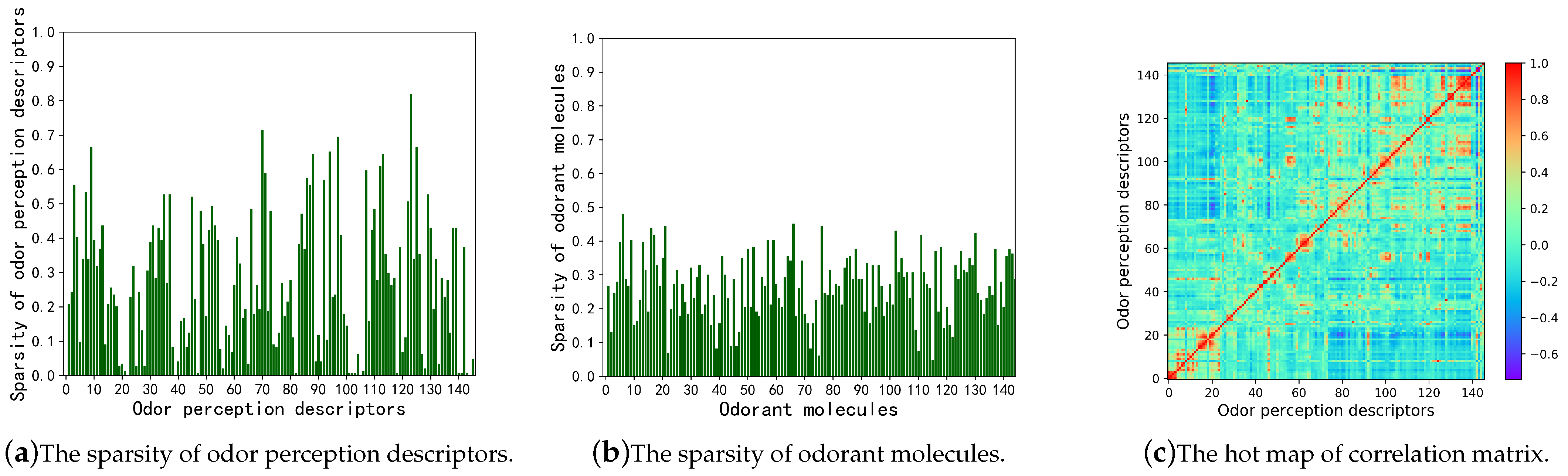
The statistics of the dataset could affect model performance. Therefore, two kinds of statistics of odor perceptual data were analyzed: sparsity and Pearson correlation matrix. The prominent characteristic of odor perceptual data is sparsity. If most elements of an odor perceptual vector are 0, it will affect the chance of becoming a clustering-center odor perception descriptor and the accuracy of its prediction. The sparsity for the Dravnieks dataset is 26.71%, which is much denser than the other odor perceptual datasets [
46]. The average perceptual rating of all odor descriptors is 3.26. The maximum sparsity of an individual odor perceptual descriptor is 81.94%, which corresponds to “fried chicken”, and the minimum is 0, which corresponds to “aromatic”, “woody, resinous”, “sharp, pungent, acid”, “heavy” and “warm”. The detailed distributions of sparsity for odor descriptors are shown in
Figure 5a. The numbers on the horizontal axis represent the 146 odor perception descriptors applied in the Dravnieks Dataset (please see
Supplementary S1).
In particular, the sparsity range of more than 85% of odor perception descriptors is 0 to 0.5. The sparsity of recapitulatory odor perceptual descriptors, such as “sweet”, “perfumery”, “floral”, “fragrant”, “paint”,” sweaty”, “light”, “sickening”, “cool, cooling”, “aromatic”, “sharp, pungent, acid”, “chemical”, “bitter”, “medical”, “warm”, and “heavy”, are below 0.1.
The distribution of sparsity of molecules is reported in
Figure 5b. The numbers on the horizontal axis represent the 144 odorants of the Dravnieks Dataset (please see
Supplementary S2). The sparsity of every molecule is lower than 0.5. The results shown in
Figure 5a,b demonstrate that the Dravienks dataset is much dense.
Pearson correlation coefficients between every two 144-dimensional odor perception descriptor vectors were calculated, as shown in
Figure 5c. The numbers 1 to 146 on the horizontal axis represent 146 odor perception descriptors(please see
Supplementary S1). It means that some odor perceptions have relatively high correlation coefficients with other odor perceptions for the correspondence between numbers and odor perception descriptors. Therefore, these odor perceptions might be redundant and could be inferred from other odor descriptors.
3.2. Stability Analysis of the Identification Framework for POPDs and NPOPDs
The stability analysis of the proposed identification framework’s results is conducted. This framework comprises the disjunctive model based on clustering algorithms and the validation model based on multi-output regression models. The multi-regression model is one of the three classical regression models: Ridge, LASSO, ElasticNet model, so the results of the validation model is stable, and the stability of this framework only relies on the disjunctive model. The stability of the disjunctive model’s results is affected by the random initialization of the clustering algorithms. To this end, the clustering algorithms are executed many times to obtain the candidate odor perception descriptors. The CCOPDs are obtained by an updating strategy based on CT and frequency constraints to ensure the disjunctive model results’ stability, as described in
Section 2.2.1.
The fewer the number of clusters is, the greater the fluctuation of the selected CCOPDs are. A higher CT could lead to the greater flexibility of CCOPDs. Hence, the stability of 10 CCOPDs with a CT of 1.0 was investigated.
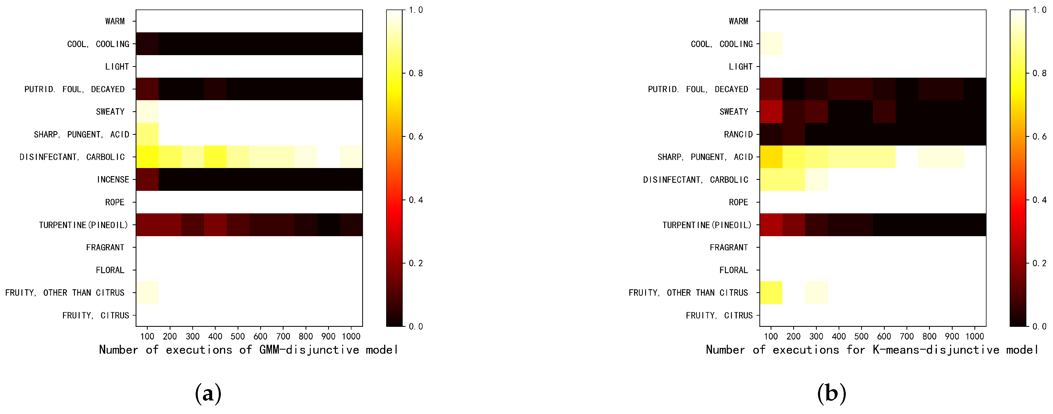
Precisely, the clustering algorithms were executed for 100, 200, 300, 400, 500, 600, 700, 800, 900, and 1000 times to obtain the candidate CCOPDs. The CCOPDs were then derived by the updating strategy based on the constraints of CT and frequency. For each of the ten numbers of the execution times for the clustering algorithms, the disjunctive model was implemented 30 times. The results are shown in
Figure 6.
It can be observed that as the number of the execution times of the clustering algorithms increases, the results of CCOPDs converge, indicating the effectiveness and stability of the disjunctive model. When the number of execution times of clustering algorithms reaches up to 1000, the results of the 30 implementations of the disjunctive models are the same. That is, the same ten CCOPDs are selected with a probability of 1. Hence, in the rest of this paper, all the results are obtained under the 1000 executions of the clustering algorithms. It should be noticed that the clustering algorithm is only used to select out the CCOPDs. After 1000 executions of the clustering algorithm and the updating strategy, the disjunctive models’ results are no longer the clustering algorithms’ results.
As shown in
Figure 6, 14 odor descriptors were chosen as the CCOPDs for GMM-disjunctive and K-means-disjunctive models, and 13 out of these 14 descriptors were overlapped. The singular one was “rancid” for the K-means-disjunctive model and “incense” for the GMM-disjunctive model, respectively. Nine out of 10 CCOPDs obtained in these models are the same, i.e., “fruity, citrus”, “fruity, other than citrus”, “floral”, “fragrant”, “rope”, “disinfectant carbolic”, “sharp pungent, acid’, “light”, and “warm”. The other odor descriptor is “sweaty” for GMM-disjunctive model and “cool, cooling” for K-means-disjunctive model. This subtle difference is due to the similarities between these two algorithms. K-means is a particular case of GMM with an isotropic covariance matrix. As the number of clustering centers increases, the results of these two algorithms are still different.
3.3. CCOPDs Derived from Disjunctive Model
Although the number of clustering centers is set between 10 and 100, the CT will affect the actual number of CCOPDs or the clustering center number. When the CT is below 0.8, the actual number of CCOPDs cannot reach 100. The maximum numbers of the CCOPDs for each CT of these two disjunctive models are presented in
Table 1.
The results of the CCOPDs of these two disjunctive models under CTs of 0.5, 0.65, 0.8, and 1.0 are presented in
Figure 7 for illustration. The horizontal axis represents 146 odor perception descriptors (please see
Supplementary S1), and the verticle axis represents the number of CCOPDs. The black blocks represent the CCOPDs. It is shown that some descriptors, such as “warm” and “fruity”, are always chosen as the CCOPDs. Some descriptors, such as “dill”, “woody, and resinous”, are never selected even if the cluster number reaches 100. For some other descriptors, their status of being chosen changes with the cluster numbers.
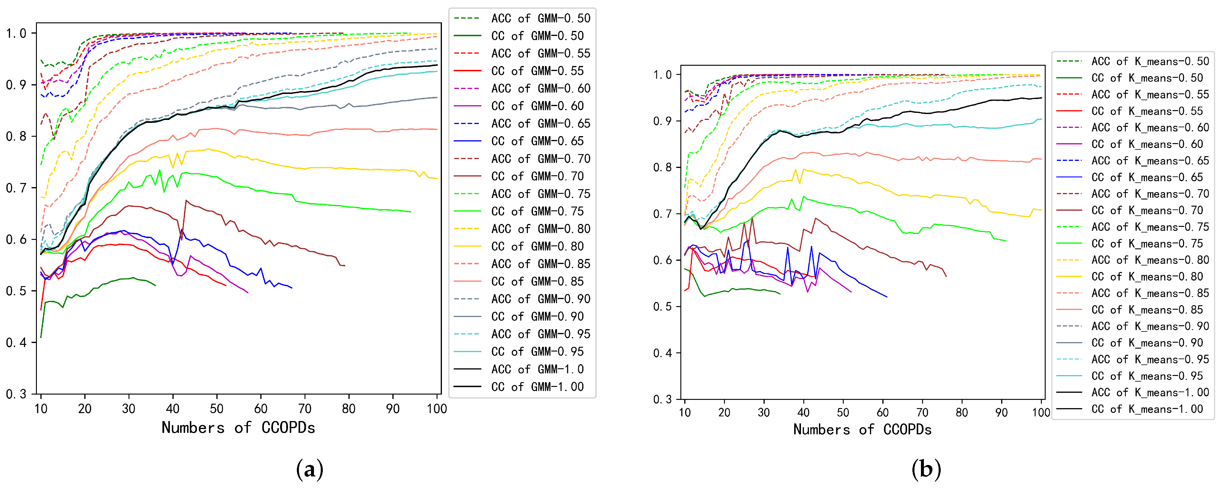
To investigate the coverage of these CCOPDs, CCs and ACCs for both disjunctive models with different CTs were calculated, and the results are presented in
Figure 8. As shown in
Figure 8a, for the GMM-disjunctive model, when the clustering center number is smaller than 30, both CC and ACC increase quickly. For the ACC, when the CTs are above 0.65, the converging rates of ACCs slow down. 0.65 is the critical CT to make the ACCs converge to 1 at high speed. When the CTs are below 0.8, CC will decrease slightly as the clustering center number increases. The level of 0.8 happens to be the critical CT for the number of cluster centers to reach 100, as shown in
Table 1. Similar conclusions can be drawn from the K-means-disjunctive model, as shown in
Figure 8b. It implies the CCs could affect the results of the disjunctive model.
3.4. Performance of Combinational Models and POPDs Identified
A predicting metric threshold must be set to discriminate the predictable and unpredictable odor perception descriptors from the NCCOPDs. If the predicting performance of the NCCOPDs is above the predicting metric threshold, it will be classified as the predictable odor perception descriptors. Otherwise, it is unpredictable and will be identified as a POPDs. The numbers of NPOPDs, namely the predictable odor perception descriptors, determined by these combinational models under different predicting metric thresholds are shown in
Figure 9.
Specifically, the grid search approach was applied in the six combinational models respectively for the hyperparameter K, i.e., the number of clustering centers. The maximum number of predictable odor perception descriptors with different CTs under different predicting metric thresholds are obtained, as shown in
Figure 9. The horizontal axis represents the other hyperparameters of the disjunctive model, namely, the CTs. As shown in
Figure 9a–c, 0.7, 0.8, and 0.9 are the predicting metric thresholds, respectively.
For each performance metric threshold, the champion model is the one obtaining the largest number of predictable odor perception descriptors among the six combinational models. For the performance metric threshold of 0.7, there are two optimal models, one is the K-means-ElasticNet model with a CT of 0.65, and the other is the GMM-ElasticNet model with a CT of 0.55. The maximum number of predictable odor perception descriptors is 71, as shown in
Figure 9a. For the performance metric threshold of 0.8, the optimal model is the K-means-ElasticNet model with a CT of 0.65. The maximum number of predictable odor perception descriptors is 51, as shown in
Figure 9b. For the performance metric threshold of 0.9, there are two champions. One is the GMM-ElasticNet model with a CT of 0.8; the other is the GMM-LASSO model with a CT of 0.7. The maximum number of predictable odor perception descriptors is 22, as shown in
Figure 9c. To summarize, the lower the predicting threshold, the more POPDs are obtained.
As expected, the ElasticNet-based model outperforms the other regression-based models in most configurations, and the LASSO-based model is better than the Ridge-based model due to its feature selection ability. When the CTs are above 0.8, the performance of these models will drop rapidly. It shows that the clustering centers are concentrated in certain areas, and the distances among them are short. Sparse regions are not involved, and supplementary information among different clusters could not be utilized, leading to undesirable results. When the CTs are below 0.6, too many isolated odor perceptions with a little relationship with the others are chosen as clustering centers. It also leads to poor prediction performance. Consequently, the disjunctive model’s CT must take an appropriate value and not too large or too small. The results show the effectiveness of the CTs on the identification framework. Besides, the high predicting metric threshold corresponds to the high CT of the disjunctive model.
Considering that prediction correlation coefficients lower than 0.7 were reported in most state-of-the-art literature, 0.8 was set as the critical value for separating the predictable and unpredictable odor perceptions. The optimal CT, the optimal number of CCOPDs, the maximum number of predictable odor perception descriptors, the optimal number of CCOPDs, and the optimal number of unpredictable odor perception descriptors for all the six combinational models with the predicting metric threshold of 0.8 are summarized in
Table 2.
As shown in
Table 2, the optimal CTs for all the combinational models is around 0.65, and it indicates that the internal relations among different odor perceptions are exploited exhaustively under a medium CT. Besides, the optimal numbers of CCOPDs of all the combinational models are around 40. By comparison, the K-means-ElasticNet model with a CT of 0.65 is the final winner, referring to as the optimal configuration.
The identification results of POPDs and NPOPDs are presented in
Figure 10. There are 51 NPOPDs and 95 POPDs, and the POPDs consist of 41 CCOPDs and 54 unpredictable odor perception descriptors. The 54 unpredictable odor perception descriptors could be regarded as isolated points due to their unpredictability. Moreover, the validation models mapping CCOPDs to NPOPDs, revealing the complicated relationship among these odor perceptions.
3.5. Relationship between Predicting Performance and Cluster Numbers for Optimal Configuration
The combination of K-means and ElasticNet regression with a CT of 0.65 is the optimal configuration. The relationship between the predicting performance and the cluster numbers
K was investigated in this configuration. Some predictable NPOPDs and unpredictable POPDs were selected for this purpose. The relationship between the predicting performance of these odor perception descriptors and the number of clusters ranging from 10 to 61 was investigated. The results are presented in
Figure 11.
As shown in
Figure 11a, the predicting performance of some predictable NPOPDs, such as “lemon”, “orange”, and “sweet”, is relatively stable, achieving a correlation coefficient above 0.9 for all the cluster numbers. On the contrary, when the number of clusters is small, the predicting performance of the other three NPOPDs, namely “apple (fruit)”, “cologne”, and “cherry”, are inadequate. As the number of clusters increases, the prediction performance will improve, especially for “apple (fruit)”. It should be noted that the correlation coefficient 0 is actually “nan”. Due to the simplicity of these models, the predicting values of some odor perceptions remain unchanged. Therefore, the correlation coefficients between the predicting values and the original labels would be “nan”. Similar conclusions are obtained for the unpredictable POPDs in
Figure 11d–f. It should be noted that some of them are predicted with a smooth correlation coefficient, and it implies that these odor perceptions, such as “burnt candle” in
Figure 11f, are singular points in the odor perceptual space and have little relationship with most other odor descriptors. In contrast, as shown in
Figure 11d, the predicting performance of “cooked vegetables” and “stale tobacco smoke” increases with the number of clusters and reaches a high value above 0.8. It shows that there is a complicated relationship between these odor perceptions and others. However, to minimize the total number of POPDs, a compromise is needed to classify odor descriptors corresponding to these odor perceptions as the NPOPDs.
3.6. Effect of Data Sparsity on Model Predicting Performance
Considering that sparsity is a significant characteristic of odor perceptual data, the impact of data sparsity on model performances was investigated. The investigation was implemented in the optimal configuration, i.e., the K-means-ElasticNet regression with a CT of 0.65. Because the number of clustering centers is between 10 and 61, there are 52 models in total under the optimal configuration. The optimal model refers to the model with 41 clustering centers under the optimal configuration. Specifically, the investigation was conducted in two scenarios. One was based on the best predicting performance of each odor descriptor obtained under the optimal configuration when the number of clustering centers varied from 10 to 61. The predicting performances of all the 146 odor perception descriptors were involved. The other scenario was based on the optimal model with the optimal cluster number of 41 under the optimal configuration, and the predicting performances of the other 105 non-clustering-center odor perceptions were involved. The results are shown in
Figure 12,
Figure 12a for the former scenario, and
Figure 12b for the latter scenario.
As shown in
Figure 12a, six odor perceptions, “fruity, citrus”, “fruity other than citrus”, “floral”, “beery”, “rope”, and “warm”, were selected as the clustering centers all the time, as marked “x” in the scatter diagram. The correlation between data sparsity and the best predicting performance of all the 146 odor perception descriptors is −0.39. In
Figure 12b, the six points with a predicting performance of 0 are odor perceptions with a constant predicting value, i.e., their predicting performance metrics cannot be calculatable. The correlation between data sparsity and predicting performance of 105 NCCOPDs in the optimal model is −0.5. These results imply that the data sparsity hurts the predicting performance, i.e., the sparser the data is, the poorer the predicting performance is.
3.7. Influence of the Pearson Correlations among Odor Perceptions on Predicting Performance
The correlations among odor perceptions are different. Some of them are highly correlated, while others are not. Hence, the influence of the correlations among odor perceptions on the predicting performance was investigated. Pearson correlation coefficients are different for every two odor perceptions, and only the large ones will significantly affect the prediction. Hence, the maximum correlation coefficients were adopted for the measurement.
The same scenarios as in
Section 3 and
Section 3.6 were adopted to investigate the influence of the Pearson correlations among different odor perceptions on predicting performance. The only difference in the scatter plots was that the horizontal axis represented each descriptor’s maximum Pearson correlation coefficient instead of the sparsity. The results of both scenarios are shown in
Figure 13. As shown in
Figure 13a,b, the correlation coefficients between Pearson correlations and predicting performance are 0.52 and 0.61, respectively. These results indicate that the Pearson correlation has a positive effect on predicting performance. It indicates that if an odor perception is closely related to others, that is, in the vicinity of the other odor perceptions, it could be accurately predicted. It reveals that the distribution of odor perceptions in the odor perceptual space is not uniform. Part of odor perceptions is clustered in some vicinities, while others were isolated points.
4. Discussion
A large number of odor perception descriptors applied in industries and academic literature is a challenging issue in the odor research community, and it hampers the odor sensory assessment in food, beverage, and fragrance industries. To tackle this issue, we propose the task of reducing the amount of odor perception descriptors, and we contrive a novel selection mechanism based on machine learning to identify the POPDs and NPOPDs. The selection mechanism aims to minimize the number of POPDs by maximizing the number of NPOPDs. The validation model in this selection mechanism builds mapping functions from the CCOPDs to the NPOPDs, revealing their relationship. Moreover, it demonstrates that the sparsity and correlation between every two odor perception descriptors dramatically impact predicting performance.
Compared with the expansion of odor vocabulary in the previous work [
19,
23,
24,
25], we propose a shrinkage strategy in this paper. Our findings demonstrate the feasibility of reducing the size of the odor vocabulary. Although the odor perception is complicated, it could be represented by a subset of odor domain-specific semantic attributes, namely, POPDs. Just like the three primary color descriptors “red”, “blue”, and “green” for visual perception. Moreover, the NPOPDs could be recovered from a weighted linear combination of the CCOPDs, just as any color can be formed by combining three primary colors.
The framework proposed in this work is based on the assumption that there are inherent links among different odor perceptions. The identification framework proposed in this paper reveals the complicated relations between POPDs and NPOPDs to some extent. It demonstrates that some odor perception descriptors could be inferred from others, and this finding is consistent with the work in [
42]. However, how to derive the general odor perception descriptors is not mentioned in [
42], while we propose a disjunctive model with an updating strategy to identifying these general odor perception descriptors that could be used to infer the NPOPDs. Therefore, our work could be taken as the prequel to work in [
42]. Moreover, it seems that the odor perceptions are not uniformly distributed in the odor perception space. Some of them are clustered together, while some of them are isolated points. That is, they have little to do with other odor perceptions. These findings are consistent with those in [
41,
44]. However, the work in [
44] focuses on the relations between the missing odor perception and the known ones, and [
41] aims to predict the odor perception from the mass spectrum of mono-molecular odorants.
Different from the approaches based on transformation, such as the work in [
31,
36,
38], a selection mechanism based on machine learning is proposed in this paper. The transformation approaches mainly concentrate on exploring odor perception space, and the axes are the mixtures of several elementary odor perception descriptors. The meanings of these axes are different from any of the elementary ones. For instance, the work in [
38] reveals ten axes of the odor perception space, which are the linear combination of several elementary descriptors. There are mainly six odor perception descriptors for the first basis vector, i.e., fragrant, floral, perfumery, sweet, rose, and aromatic. Any existing word could not denote the exact meaning of the mixture of the six odor perception descriptors. These axes could not be used directly for odor assessment. If we want to obtain the perceptual ratings of these axes, The perceptual ratings of its elementary odor perception descriptors must be obtained first. Therefore, the findings of these transformation-based approaches could not simplify the odor assessment. Moreover, there is overlap among the ten axes identified in [
38]. For example, “fragrant” is elementary of the first three axes, and it indicates that there is redundant information among these axes. By contrast, our work focuses on reducing the odor vocabulary, and a selection strategy is adopted. Hence, the original meanings of these odor perception descriptors could be reserved. As POPDs are different from each other, there is less redundant information among them. By the fewer numbers of POPDs, the odor assessment could be simplified. Only the ratings of POPDs are needed to evaluate in the odor assessment task, and the ratings of the other odor perception descriptors could be obtained through the validation models. From this viewpoint, our work is also different from the work of [
20,
35], which focuses on how to develop a standard sensory map of perfume product. The reduced number of odor perception descriptors might also be auxiliary to the odor perception space’s research.
In summary, a shrink strategy of odor vocabulary is proposed. The relations between different odor perceptions are revealed by the mapping functions obtained from the validation model in this work.
Several limitations of the present work and further improvement need to be mentioned. This work mainly demonstrates the feasibility of reducing the size of odor vocabulary. The mapping functions determined by the validation model are learned automatically by “machine” and could not be explained clearly by human beings. The relationship between these odor perceptions and the odor perception space’s structure remains elusive for human beings. More powerful models could be adopted to reduce the size of POPDs set further. For example, multi-task learning deep neural networks could be used as the regression model to improve predicting performance, and a smaller set of POPDs could be obtained. Due to the smoothness of the predicting performance, not all the CCOPDs are helpful for the prediction. Some feature selection algorithms may improve the predicting performance and speed up the computation. The NLP techniques could be introduced to provide supplementary information among different odor perceptions. Besides, it is possible to enlarge the odor psychological dataset to capture more and more information among different odor perceptions. More effective processing of sparsity of odor perceptual data also requires a better solution.


