Article

3D Acoustic Mapping in Automotive Wind Tunnel: Algorithm and Problem Analysis on Simulated Data

by
Gianmarco Battista
1,†,
Paolo Chiariotti
2,†,
Milena Martarelli
1,*,†,
Paolo Castellini
1,†,
Claudio Colangeli
3,† and
Karl Janssens
3,†
1
Department of Industrial Engineering and Mathematical Sciences, Università Politecnica delle Marche, 60100 Ancona, Italy
2
Dipartimento di Meccanica, Campus Bovisa Sud via La Masa 1, 20156 Milano, Italy
3
Siemens Industry Software NV, Interleuvenlaan 68, 3001 Leuven, Belgium
*
Author to whom correspondence should be addressed.
These authors contributed equally to this work.
Appl. Sci. 2021, 11(7), 3241; https://doi.org/10.3390/app11073241
Submission received: 23 February 2021 / Revised: 30 March 2021 / Accepted: 31 March 2021 / Published: 4 April 2021

Abstract

:
Localization and quantification of noise sources are important to fulfill customer and regulation requirements in a such competitive sector like automotive manufacturing. Wind tunnel testing and acoustic mapping techniques based on microphone arrays can provide accurate information on these aspects. However, it is not straightforward to get source positions and strengths in these testing conditions. In fact, the car is a 3D object that radiates noise from different parts simultaneously, involving different noise generation mechanisms such as tire noise and aerodynamic noise. Commonly, acoustic maps are produced on a 3D surface that envelopes the objects. However, this practice produces misleading and/or incomplete results, as acoustic sources can be generated outside the surface. When the hypothesis of sources on the model surface is removed, additional issues arise. In this paper, we propose exploiting an inverse method tailored to a volumetric approach. The aim of this paper is to investigate the issues to face when the method is applied to automotive wind tunnel testing. Two different kinds of problem must be considered: On the one hand, the results of inverse methods are strongly influenced by the problem definition, while, on the other hand, experimental conditions must be taken into account to get accurate results. These aspects have been studied making use of simulated experiments. Such a controlled simulation environment, by contrast to a purely experimental case, enables accurate assessment of both the localization and quantification performance of the proposed method. Finally, a set of scores is defined to evaluate the resulting maps with objective metrics.

1. Introduction

The acoustic performance of vehicles is crucial for automotive industries, both from a legislative point of view and for the quality perceived by customers. Three main sources of noise can be identified in a car: engine, structure-borne, and airborne. With the advancement of electric engines, the latter two sources of noise are gaining increasingly more importance and deserve to be studied in more detail. Wind tunnel tests allow performing measurements in controlled operational condition. Generally, one or more microphone arrays are installed in wind tunnels in order to acquire pressure data as input for acoustic mapping techniques, also called acoustic imaging. A detailed review of these techniques is available in [1]; they are an important tool for engineers that is exploitable during the design and testing phase to localize and rank the acoustic sources in vehicle exterior noise source identification. Two non-trivial challenges must be faced when mapping acoustic sources on three-dimensional objects. The first issue is the masking effect that the object itself produces between some sound sources and some microphones. Considering this effect in the propagation model could be prohibitive, as it involves complex scattering and the transmission of sound waves. The other aspect regards the choice of the spatial region to map. Commonly, the region of interest (ROI) chosen is a surface that represents the object. This could produce inaccurate results, as sound sources could be located outside the surface, especially the aeroacoustic ones. For this reason, in this work a volumetric three-dimensional approach is adopted.
Unfortunately, real experiments do not allow the complete control of all parameters and phenomena (especially aeroacoustic ones), thus the necessity of evaluating each effect singularly arises. Therefore, simulated virtual experiments, reproducing a realistic measurement setup in a wind tunnel, have been produced to study the effect of these issues on acoustic maps. Moreover, the simulations allow us to compare the source retrieved with the exact ones in terms of localization and sound power quantification.
The choice of acoustic mapping technique is conditioned by the volumetric mapping approach. Indeed, on the one hand, a good spatial resolution is required in all directions and, on the other hand, the problem size (i.e., the number of potential sources in the ROI) hugely increases. One acoustic imaging method is Conventional Beamforming (CB), but the poor spatial resolution in the radial direction from the array center and the high sidelobe level make it not well suited for volumetric maps. Another method is based on computationally expensive deconvolution algorithms like CLEAN-PSF or CLEAN-SC [2] that exhibit higher computational time than CB and comparable accuracy in terms of source localization. However, Sarradj [3,4] showed how to produce good volumetric maps with CLEAN-SC using different steering-vector formulations. Porteous et al. [5] described and compared several techniques for volumetric mapping with two planar arrays oriented on orthogonal planes. The exploitation of multiple arrays, the so-called “multiplicative beamforming” principle, has been proposed in literature in different formulations and array/source configurations, but always with the purpose of enhancing the computed acoustic map and reducing the effect of side-lobes and artifacts in the acoustic image [6,7,8]. Another powerful deconvolution approach is DAMAS and its variants [9]. These techniques enable achieving good spatial resolution and accuracy in all directions, but they are computationally expensive (especially for the Point Spread Functions calculation phase) and often not compatible with the problem size of volumetric mapping. An application of DAMAS 3D was proposed in [10], where the focusing ability of beamformers with planar arrays was evaluated both in lateral and longitudinal directions. The DAMAS capability of returning correct source locations and strengths was assessed in relation to frequency, source separation distance, and array design. In order to achieve high spatial resolution in all directions, four planar arrays surrounding the object in the wind tunnel test section were exploited in [11]. Acoustic data were processed with different mapping techniques. Padois et al. [12] compared the performances and the computation time of different acoustic imaging methods applied to data achieved with one planar array and with two arrays placed on orthogonal planes. Ning et al. exploited Compressed Sensing techniques to get volumetric maps [13]. Battista et al. described how to obtain accurate high-resolution maps with inverse methods using a single planar array [14]. In that paper, different approaches were compared such as Covariance Matrix Fitting (CMF) [15] with different solvers and an Equivalent Source Method (ESM) based on Iteratively Re-weighted Least Squares (IRLS) and Bayesian Regularization (BR) [16,17]. Due to its relatively low computation demand, ESM has been chosen for challenging applications such as an aircraft model in a wind tunnel [18]. First, the method was tested on simulated data to evaluate its ability in terms of localization and dynamics, and then the results on experimental data were shown.
The aim of this paper is to identify the challenges in the application of acoustic mapping techniques to automotive wind tunnel testing and to evaluate the effect of different testing and processing parameters on the resulting noise source map. The experimental aspects studied are the use of a single or dual planar array and the effect of different masking levels and Signal-to-Noise Ratios (SNR). The processing parameters considered are the definition of the ROI and its discretization with potential sources, which heavily affect inverse method performances and computational time. In order to objectively evaluate the quality of the maps obtained, a set of scores has been defined.
The paper is organized as follows. Section 2 describes the inverse acoustic problem and the data preprocessing, and Section 3 illustrates the strategies to achieve the volumetric acoustic maps. The virtual experiment synthesized to perform a sensitivity analysis in relation to experimental and numerical factors (e.g., noise and calculation volumetric point grid resolution) is described in Section 4. The results of the sensitivity analysis are reported in Section 5. Section 5 shows the results obtained on a simulated test case which considers all the effects present in a real experiment. Finally, Section 6 draws the conclusions from the parametric study conducted.

2. Volumetric Acoustic Inverse Problem Formulation and Data Preprocessing

2.1. Acoustic Direct and Inverse Problems

In frequency domain, the discrete acoustic direct problem can be described, for each frequency, by the following linear relationship:
G q = p ,
where q is the vector of complex source strengths of S elementary sources in assumed positions, p is the vector containing the complex pressures measured at M receiver locations, and the complex matrix G represents the acoustic propagation matrix. The direct acoustic problem identifies the calculation of p for given q and G . This is a well-determined problem having a unique solution. Conversely, the calculation of q for given G and p is the inverse acoustic problem, which results to be ill-posed in Hadamard sense, i.e., existence, uniqueness, and stability of solution are not guaranteed [19]. For this reason, the estimated source coefficients q ^ ( T ) depend on the assumptions and a priori information about the source distribution. A detailed review about different inverse operators is provided by Leclère et al. [20,21]. In the application of inverse problems for volumetric acoustic map reconstruction, three critical issues emerge: (i) the influence of potential sources located at very different distances from the array center, (ii) limited spatial resolution in the radial direction from the array center, and (iii) increase in the number of potential sources notwithstanding that a few of them significantly contribute to the acoustic field. These issues must be taken into account and must be properly considered in conjunction with all other challenges involved in acoustic mapping techniques. Note that these may be present in any acoustic imaging context, but they are severely enhanced in volumetric applications.

2.2. Pressure Data Preprocessing

Before describing how to obtain a solution for the inverse problem, it is worth addressing in which form measured data can be used to set the problem. An inverse problem is solved for each spectral line, therefore frequency content must be extracted properly from time data. The term p can be the vector of Fourier transform of the pressure time histories measured by the microphones. However, in aeroacoustic measurements, pressure data are generally processed to estimate the Cross Spectral Matrix (CSM) P , given the random nature of aeroacoustic noise. One possible strategy for source mapping is to extract coherent source components from CSM, solve an inverse problem for each of them, and then obtain the complete acoustic map summing all contributions. This aspect is not strictly linked to 3D mapping, but separation of coherent sources from noise helps to better condition the inverse problem, thus requiring less regularization. Suzuki [17] proposes to decompose CSM in eigenmodes e i and use them as measured data:
G q i = e i i = 1 , , M 0
where M 0 M is the number of expected components. Therefore, the generic vector of complex pressure p is replaced by each eigenmode in turn, and the total map is obtained from the energetic sum of all component maps q ^ i . The eigenmode decomposition is based on the property of CSM that is Hermitian and non-negative definite. Therefore, it can be decomposed as
P = E v e c E v a l E v e c H ,
where E v e c is a unitary matrix of M orthonormal eigenvectors and E v a l is a diagonal matrix containing the corresponding eigenvalues. It is possible to define the eigenmode e i as the eigenvector, including its amplitude:
e i = e v a l , i e v e c , i i = 1 , , M
where e v e c , i is the i - t h eigenvector and e v a l , i is the corresponding eigenvalue. Under the constraint of orthogonality, each eigenvector represents a coherent signal across the microphones. In this paper, the eigenmode decomposition is used, but any other method to extract a source component from CSM can be used. An example of this is provided by Battista et al. [18] for aeroacoustic applications, where CLEAN-SC is proposed as a CSM decomposition tool.

3. Volumetric Acoustic Mapping Based on IRLS

3.1. IRLS Solution Strategy

Inverse problems are generally underdetermined because the number of microphones (i.e., the number of equations) is limited by practical aspects, while the number of potential sources (i.e., the number of unknowns) is often larger, in particular when dealing with three-dimensional volumetric acoustic mapping. Therefore, to find a particular solution, some assumptions on its characteristics must be done. Two kinds of assumptions are discussed hereinafter: solutions with minimum energy (least-square solutions) and solutions with minimum number of non-zero elements (sparse solutions).
A straightforward approach for solving Equation (1) is the Moore–Penrose pseudo-inverse, which is a generalization of inverse matrix to rectangular matrices. In the case of an underdetermined system, this inverse operator returns the solution with the smallest L 2 -norm among those satisfying the linear equations in Equation (1):
q ^ = arg min q q 2 2 subject to G q = p .
From a physical point of view, this represents the minimum energy solution that exactly matches the measured pressure data. This is often referred to as a naïve solution because errors in the propagation model and/or noise in measured data (providing variations on G and p , respectively) lead to unstable solution. The solution of the inverse problem can be written as
q ^ = G H ( G G H ) 1 p = V S 1 U H p = k = 1 M u k H p s k v k
where the superscript H stands for the conjugate transpose. For the last two expressions, Singular Value Decomposition (SVD) of direct operator G = U S V H has been used; S is a real diagonal matrix containing the singular values s k > 0 in decreasing order, while U and V are two unitary matrix whose columns u k and v k form two orthonormal bases. Noise in the measured data and propagation modeling errors have an effect on Fourier coefficients, which is amplified when divided by singular values (especially the smallest ones).
A common approach to overcome this problem and calculate a regularized solution is the Tikhonov Regularization [22]. This approach consists in the following minimization problem:
q ^ ( η 2 ) = arg min q G q p 2 2 + η 2 q 2 2 .
This is a joint minimization of the solution norm q 2 2 and residuals norm G q p 2 2 , where the regularization parameter η 2 0 controls the trade-off between the amplitude of the solution and the fitting error. The regularization parameter is used to adjust the cut-off on singular values, preventing the amplification of noise in the inversion operation, thus stabilizing the solution. A more general approach to inverse acoustic problems has been proposed by Antoni [23], where Bayesian inference has been exploited for developing a method which is able to (i) identify the optimal basis functions which minimize the reconstruction error, given the topology of the specific acoustic problem; (ii) include a priori information on source distribution to better condition the problem and ease the reconstruction task; and (iii) provide a robust regularization criterion. The idea at the basis of the Bayesian approach for acoustic source reconstruction is to endow all unknown quantities with a probability density function (pdf), instead of considering them as deterministic. Bayesian regularization provides different strategies to estimate η 2 directly from data, propagator, and a priori information [24]. All of them lead to a particular cost function to minimize with respect to the regularization parameter. These cost functions share the property of having a unique global minimum in most application conditions, thus giving a reliable estimation of the amount of regularization needed. The cost function chosen here returns the value with the maximum probability of occurrence, i.e., the maximum a posteriori estimation of η 2 :
J M A P ( η 2 ) = k = 1 M ln ( s k 2 + η 2 ) + ( M 2 ) ln 1 M k = 1 M | y k | 2 s k 2 + η 2
η M A P 2 = arg min η 2 J M A P ( η 2 ) .
The solutions based on energy minimization described above suffer similar issues to those of beamformers. In fact, the L 2 -norm minimization mechanism spreads the energy of single source into several potential sources [17]. In fact, even a single point source is mapped into a “main lobe” and other artifacts, thus leading to bad spatial and poor dynamics. For these reasons, they are not well suited for three-dimensional acoustic mapping. In addition, it has been proven to suffer of severe underestimation of source strength [16] especially when dealing with volumetric imaging. In fact, it so happens that the size and shape of the real sources do not change, while only the ROI increases its size; therefore, its discretization requires more potential sources to keep the same spatial resolution. This consideration suggests the hypothesis of sparsity of the source field, which means that it can be approximated by few non-zeros elements in a given representation. In fact, the basis adopted in the direct operator is crucial when sparse representation is sought, as the hypothesis can be fulfilled in some representation and not in others [21]. In this paper, only monopoles are used to build the matrix G , but other elementary sources can be adopted (dipoles, plane waves, spherical harmonics, etc.). It is known that a priori assumptions such as sparsity and choice of basis are mandatory to achieve satisfactory results in source quantification. Sparsity can be enforced by minimizing the L p -norm of solution jointly with the fitting error, thus having the following problem:
q ^ ( η 2 , p ) = arg min q G q p 2 2 + η 2 q p p
with 0 p < 2 . True sparse representation of the source field is achieved when p = 0 . Unfortunately, the exact solution of this problem is known to be NP-hard. A method to get a sparse solution is the Iteratively Re-weighted Least Squares [25], and it is the method adopted in this work. This approach is exploited in several acoustic imaging techniques, for example, Generalized Inverse Beamforming (GIBF) [17], Equivalent Source Method (ESM) [16], or Iterated Bayesian Focusing (IBF) [26]. These methods differ from each other in the hypotheses and in other algorithmic aspects. The method described in this paper shares the theoretical bases with the aforementioned ones and is adapted to volumetric mapping. The optimization problem of Equation (10) has no general analytic solution but can be solved iteratively using the following consideration:
q p p = n = 1 N | q n | p = n = 1 N w s p , n 2 | q n | 2 = W s p q 2 2 .
Each iteration is a regularized weighted least-square problem in the general Tikhonov formulation or the equivalent Bayesian one, thus leading to the IRLS approach, as the L p optimization is achieved making use of weighted least squares and a diagonal weighting matrix W s p to converge to a sparse solution. Weights depend on the result of the previous iteration according to the following expression:
w s p , n ( i t ) = q ^ n ( i t 1 ) p 2 2
where the superscript ( i t ) is the current iteration and w s p , n is the n - t h generic diagonal element. As the exponent of weights is negative for p < 2 , division by null elements must be somehow avoided to have an invertible weighting matrix. This algorithm boils down to an iterative procedure that is a fixed point for Equation (10) and converges to global minimum for convex problems ( p 1 ) or to a global or local minimum for non-convex problems ( 0 p < 1 ).

3.2. IRLS Procedure

The IRLS procedure to solve the inverse acoustic problem can be formalized with the following expression:
q ^ ( i t ) = F q ^ ( i t 1 ) , W ( i t ) , η 2 ( i t ) , G ( i t ) , p , p .
where the function F is given by the inverse operator coming from Equation (10). From a Bayesian point of view, this method can be seen as an Expectation-Maximization algorithm which converges to a maximum a posteriori solution [27]. The procedure is the following:
  • Set the weighting matrix for the current iteration W ( i t ) = W 0 W s p ( i t ) . Calculate W s p ( i t ) using Equation (12), with W s p ( 1 ) = I . Both matrices are normalized, before their multiplication, such that W 0 = W s p ( i t ) = 1 .
  • Estimate the regularization parameter η 2 ( i t ) for the current iteration using Equation (9).
  • Calculate the solution q ^ ( i t ) and apply a threshold to discard potential sources that do not contribute significantly to the acoustic field. The set of indices n of potential sources to discard is found using the following criterion:
    n : 10 log 10 | q ^ n | ( i t ) q ^ ( i t ) < T H R d B .
    Sources (unknowns) discarded are set to zero in the final solution and the relative columns of direct operator G ( i t ) are removed for the next iterations. The same happens with the weighting matrix W ( i t ) .
  • Evaluate a convergence criterion; if not fulfilled go back to step 1; otherwise, stop the iterative procedure.
This algorithm returns a sparse approximation of the source field. A priori information introduced with W 0 can be used to penalize regions that are less likely to find sources. Padois et al. [28] proposed using a CB map for similar purposes as it provides a robust estimation of source location, despite the information being rough and smooth. However, any spatial weighting can be adopted as a priori distribution. An advantage of IRLS is that the amount of sparsity enforced on the solution can be finely tuned adjusting p. For example, in the presence of distributed/extended sources, p = 1 may be a good choice, while in presence of point sources, p = 0 is the best choice. The latter is generally the best choice for source quantification. The discarding of sources is done both to avoid the division by zero in the calculation of weights as well as to speed up the algorithm. The threshold used in this work is T H R d B = 100 dB. This value guarantees the discarding of elements that do not contribute significantly to the solution. The convergence criterion adopted here was proposed by Battista et al. in [14]:
M S R = q ^ n ( i t ) / q ^ n ( i t 1 ) ε ( i t ) = 10 log 10 M S R ( i t ) Δ ( M S R ) ( i t ) Δ 2 ( M S R ) ( i t )
where MSR stands for Mean Source Ratio, the operator · refers to the spatial average, and the operators Δ ( · ) and Δ 2 ( · ) are the backward finite differences of first and second order, respectively. This criterion can be evaluated only for i t > 2 (given the second order finite difference) and requires the solution variation to be small over three last iterations. The algorithm stops when ε ( i t ) 0.1 dB. The IRLS described in this section enables obtaining a volumetric map of sound sources using any array shape (planar, multiple planar, spherical, distributed [29], etc.) as it fulfills all requirements of the analysis discussed in the previous section. The characterization of the performance attainable with an inverse method is difficult to assess, as the results are affected by a huge number of factors.

4. Virtual Experiment

The aim of this work is to evaluate the performance that can be obtained in the context of volumetric mapping in automotive wind tunnel tests. Real experiments do not enable the user to have complete control on all parameters that influence the result. For this reason, the choice of simulated virtual experiments is made. The virtual experiment adopted in this work aims at reproducing a common aeroacoustic measurement setup in wind tunnels (WT) and related issues.

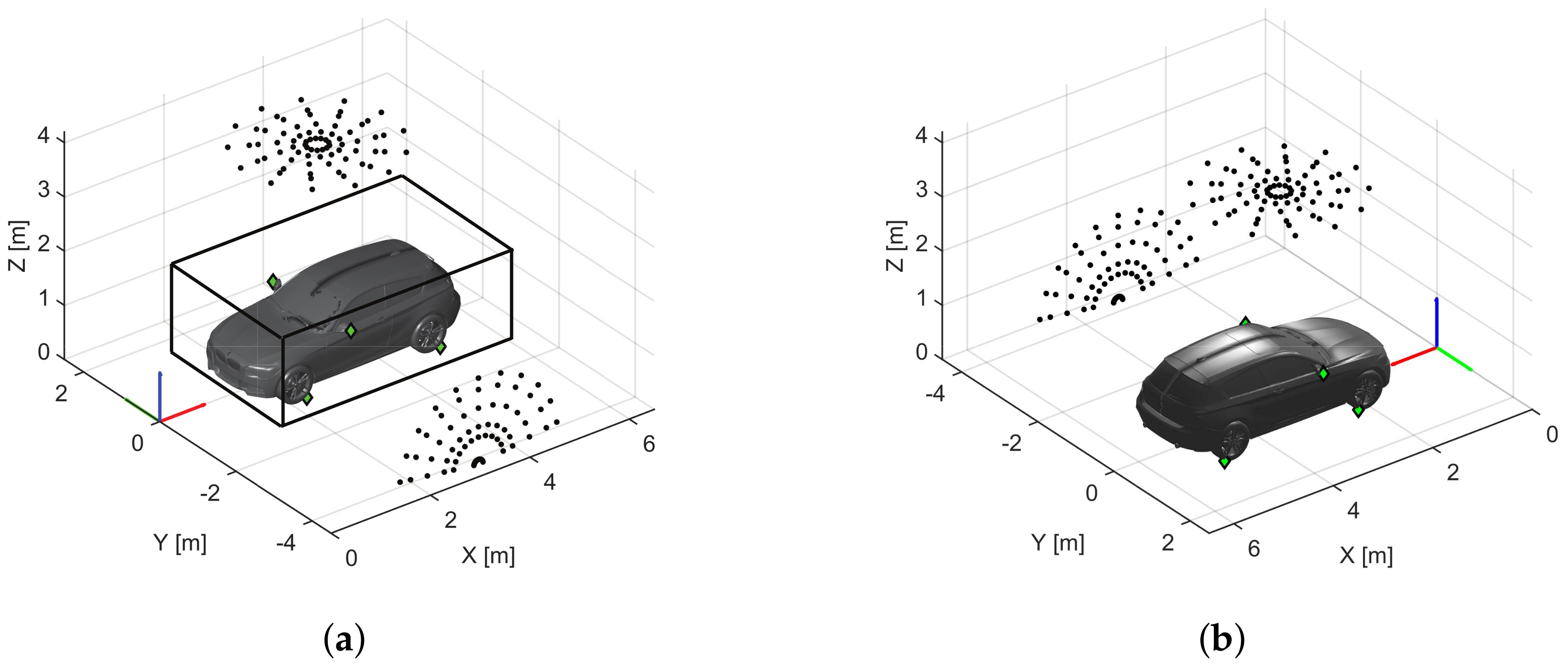
4.1. Setup Description

In order to make the virtual test realistic, we considered the actual layout at the Pininfarina WT (Orbassano, Italy). A 78-microphone wheel array is placed 4 m above the ground and a 66-microphone half-wheel array is placed on a side, 4.2 m from the median plane of the test section. Both arrays have 3 m as their maximum dimension. Figure 1 shows the arrays and the test section that allows hosting a real-size car. The flow is considered in the x-axis direction and the speed is set to 28 m/s (~100 km/h). The calculation volume is a parallelepiped of dimensions 5 m × 3 m × 1.7 m, which contains the whole car model as depicted in Figure 1a and is discretized with a regular grid of monopoles; where not specified differently, the grid step is 5 cm. In this work, only monopoles sources are considered. The elements of the G matrix are calculated as
G m n = r 0 n r m n e j k ( r m n r 0 n ) .
The terms r 0 n are the propagation distances between the reference point “0” and the location of potential sources. The reference point can be chosen arbitrarily, avoiding the coincidence with a potential source location. The terms r m n correspond to geometric distances between microphones and the potential sources in case of free-field propagation. Instead, in the presence of flow, these terms are calculated as virtual distances corresponding to the actual traveling time for a given flow field and speed of sound. In this paper, the assumption of an uniform flow in the wind tunnel is made, thus leading to the following expression for r m n [30]:
r m n = r n r m 2 C m n + C m n 2 M a 2 + 1 , C m n = ( r n r m ) · f ^ M a
where f ^ is the flow direction and M a is the Mach number.

4.2. Simulation of Microphone Signals

The virtual experiment has been parametrized in order to control the most relevant parameters affecting the acoustic field surrounding the car body. Those aspects are
  • microphone arrays used in the experiment (only the array on top or both the two arrays),
  • considering potential sources in the full volume (i.e., also inside the model) or removing a priori all of them inside the model,
  • resolution of the calculation volume point grid,
  • accounting for the masking effect due to the car body on the sources not directly “seen” by microphones, and
  • different Signal-to-Noise Ratios (SNRs) of measured data.

4.2.1. Source Simulation and Synthesis of Acoustic Pressure at Microphones

The simulated sources are S = 6 monopoles positioned as green/black diamonds in Figure 1. Two sources represent the aerodynamic noise generated by side mirrors, while the other four sources represent the trailing edge tire noise. All sources are driven with white noise, properly filtered to reproduce the typical frequency content of aerodynamic and tire noise. The filter settings are bandpass between 600 and 2000 Hz for aerodynamic noise (side mirrors sources), and bandpass between 1.3 and 3 kHz for tire noise. The sources are correlated in pairs because they are driven with the same signal: the two on left tires, the two on right tires, and the two on side mirrors. Resulting source spectra are depicted in Figure 2. Three one-third octave bands are selected for the analysis with acoustic mapping: 800 Hz, 1.6 kHz, and 2.5 kHz. In the first and in the last band, tire and aerodynamic noise are prevailing, respectively, while in the middle band all noise sources have the same level.
Source signals are propagated considering free-field propagation in a uniform flow. The speed of sound is set at 343.8 m/s. Simulated microphone signals are generated at a sampling rate of 32,768 samples/s, and contributions of each source are summed together at microphone locations. The duration of the signals is 10 s.
Uncorrelated noise on each microphone (i.e., spatially white noise) is not representative of the actual WT test conditions. Externally to the test section, radiating real sources are present. They have a well-defined spatial distribution that is also frequency-dependent. To obtain realistic simulations, real recordings of the WT background noise are used. Time signals were acquired in the real Pininfarina WT without any model in the test section at flow speed of 28 m/s, using the same array configuration used for the simulations. These signals have been used as background noise (BGN), in the synthesis of simulated signals. The simulated total pressure p t o t , m ( t ) on each microphone is obtained as follows:
p t o t , m ( t ) = p s i g , m ( t ) + G · p b g n , m ( t ) m = 1 , , M
where p s i g , m ( t ) is the contribution of all simulated sources on each microphone and p b g n , m ( t ) is the real WT noise recorded by each m - t h microphone. The desired Signal-to-Noise Ratio (SNR) is obtained by setting the proper gain G and has been calculated using microphone auto-spectra, averaged over all microphones, respectively, of simulated source signals and real WT noise signals. Once the band of interest is selected, the overall band power, P s i g and P b g n , is estimatedand G is calculated as
G = P s i g P b g n 10 ( SNR d B / 20 )
where SNR d B is the target SNR, expressed in dB. In this way, data produced have the desired overall SNR for the band of interest (not for each single spectral line).

4.2.2. Simulation of Source Masking

In the described setup, some direct source–microphone propagation paths are occluded by the presence of the model itself. Figure 3 shows which source–microphone combinations are in direct line-of-sight (LOS). In the non-line-of-sight (NLOS) condition, the propagation mechanism becomes more complex. Indeed, it involves transmission and scattering by the object. A careful reproduction of actual propagation in this condition would require a detailed knowledge of the geometry and materials of the object. In this paper, the masking effect is modeled simply using a constant Masking Attenuation factor ( M . A . ) for all microphones in NLOS condition. Therefore, each source is propagated using the free-field propagator, then NLOS microphone signals are attenuated and finally the contribution of all sources are summed together to produce time data.

5. Results of Parametric Study

Time data have been processed to estimate the CSM using Welch’s method (block size: 1024 samples, overlap: 50%, window: Hanning). The number of eigenmodes used for each analysis conducted in this work is M 0 = 10 . The maximum sparsity constraint is imposed by setting p = 0 . The reference point r 0 for the acoustic transfer function is the origin of the coordinate system. The acoustic maps represented in the figures reported in this paper are given in terms of pressure generated by each monopole at the reference point with a dynamics of 40 dB. Source strengths are also calculated from the acoustic maps, in terms of volume acceleration (m 3 /s 2 ). They are retrieved by integrating the equivalent source strengths over a sphere of radius λ centered in the source position. λ is the wavelength of sound corresponding to the frequency at which the calculation is performed (or the center frequency of the band analyzed).
In order to make an objective comparison among different cases/parameters configured in the simulation, a set of scores has been defined to evaluate the localization and quantification performance. The localization scores are as follows:
  • Identified sources. A source can be labeled as “identified” if there exists at least one equivalent source with non-null strength in its zone of interest. The set of indices n of equivalent sources to determine if a source is identified can be formalized as
    I s = n : r n r s 2 λ q n 0 , s = 1 , , S .
  • Number of sources identified ( S i d ). This simple score is formalized as the cardinality of the set that includes all indices s corresponding to non-empty sets I s :
    S i d = c a r d ( s : I s ) .
  • Identified source position ( r s , i d ). This indicator is the centroid (weighted with source powers) of the cloud of equivalent sources for each I s :
    r s , i d = n I s Q n r n n I s Q n
    where Q n = q n q n * is the power associated to each equivalent source in the map.
  • Non-dimensional distance error ( D s ). This score is defined as the geometric distance between the identified source position and the real one, normalized by the wavelength:
    D s = r s , i d r s 2 λ .
The quantification scores are as follows:
  • Power concentration ( W % ). This score indicates the sum of the power of identified sources with respect to the total power of map. It is calculated as
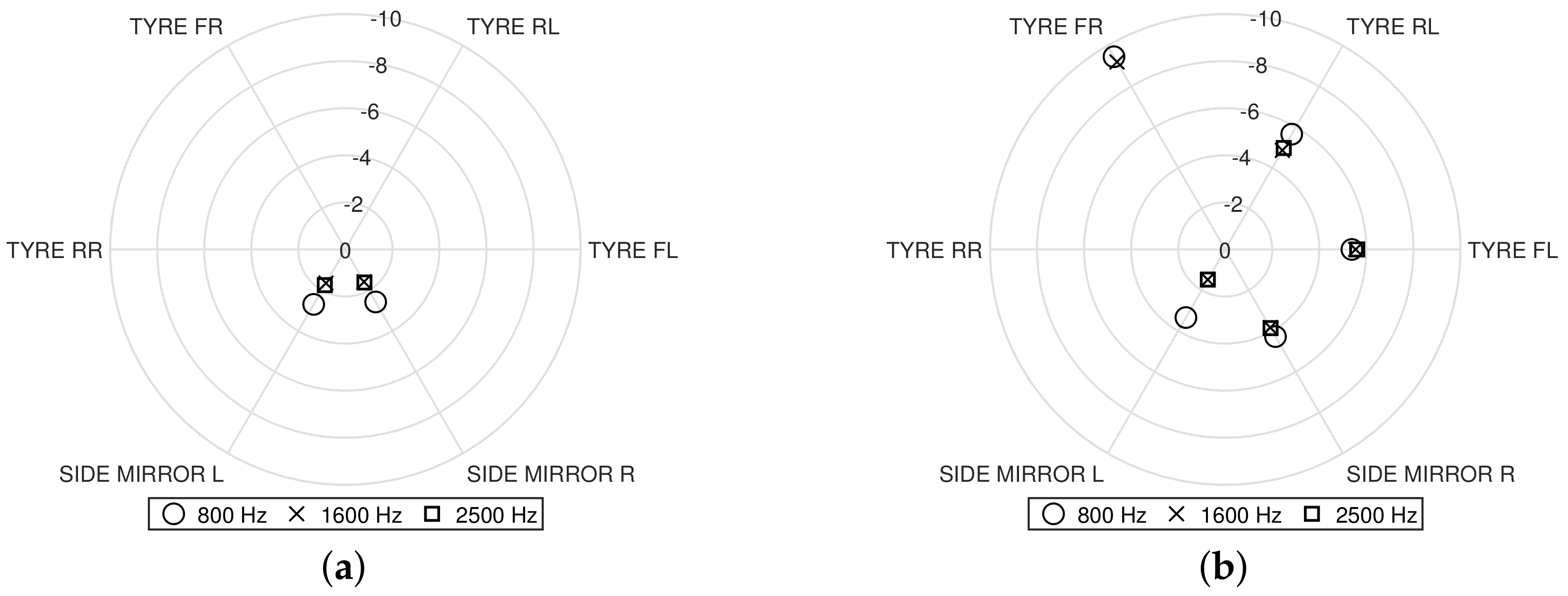
    W % = s = 1 S i d n I s Q n n = 1 N Q n .
  • Source power ratio ( W s ). It indicates the ratio of the power associated to each identified source with respect to the real source power.
    W s = l o g n I s Q n Q s , e x a c t
Power concentration is useful because it can be calculated in real applications, while the source power ratio is useful in this context to evaluate the quantification accuracy as the real power of simulated sources is known. Both localization and quantification scores must be calculated on the total map (energetic sum of all component maps). They can be calculated for each spectral line or for the whole band of analysis. In the latter case, the wavelength used is the one associated to the center frequency of the band.

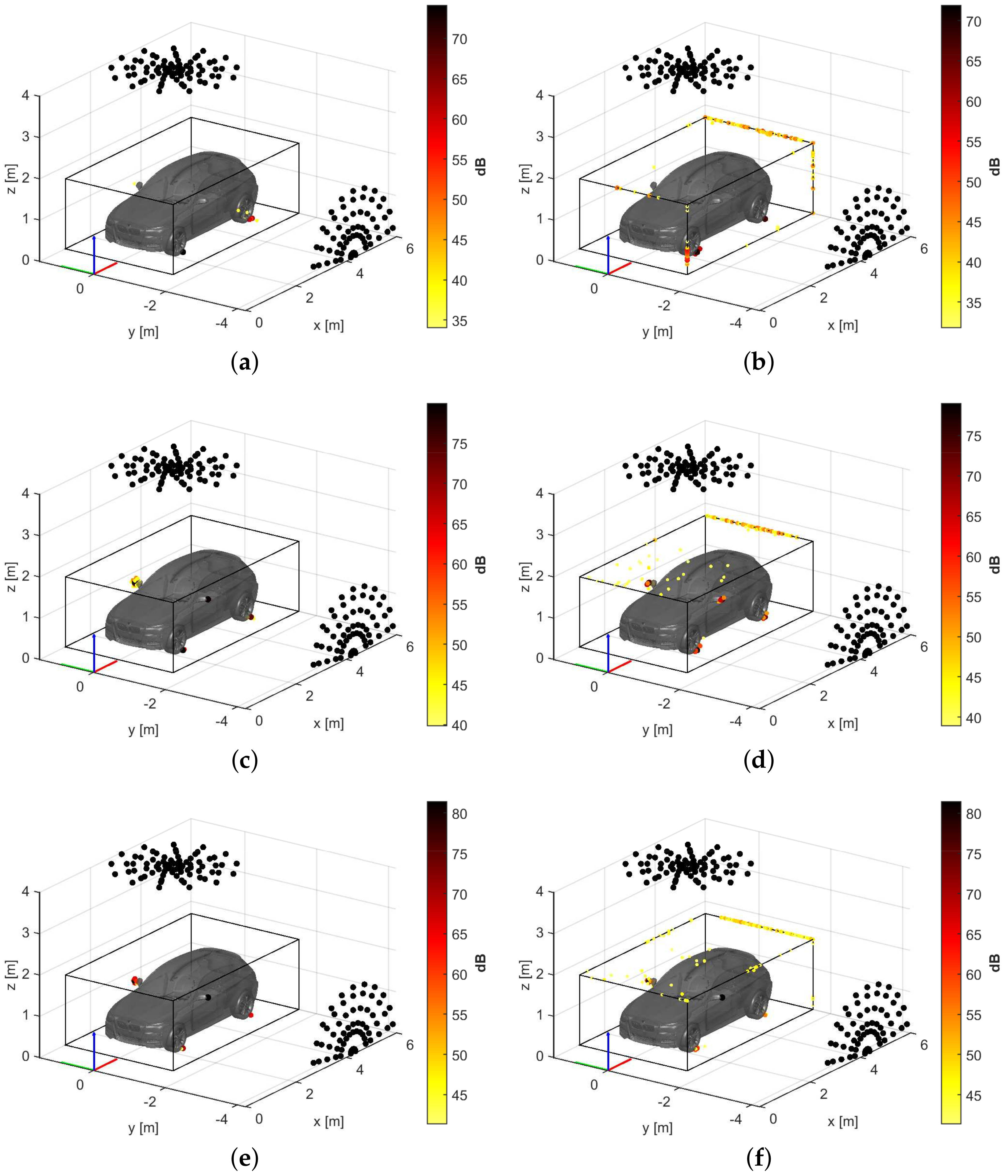
5.1. Single Array versus Multiple Arrays with Different Levels of Masking Effect

When a three-dimensional object radiates noise from some of its parts, the body itself is an obstacle for the propagation, and some sources of noise are not directly perceived from some directions. The measurement setup for acoustic mapping should account for this issue. The combined use of arrays looking at the same object from different points of view is important to identify all noise sources. Inverse methods allow using multiple planar arrays simultaneously without particular issues; the only drawback is the increment of computational cost. The simulated test cases analyzed in this section help us to understand the impact on acoustic maps of sources partially masked to the microphone array. As already said, realistic reproduction of scattering and transmission of the propagating waves by the model is a complex task. For this reason, the masking effect is simulated by means of simple attenuation of the pressure produced at microphone locations in NLOS condition by each source. No background noise is present in these simulations, and three levels of M . A . are tested: 6, 10, and 20 dB. The calculation is performed on a regular grid of monopoles with a 50 mm step that is all around the car model. All potential sources inside the car volume are removed from the calculation grid.
In Table 1, S i d in the case of single array is reported for different bands and attenuation levels. In the case that both arrays are used, all the sources are always localized. M . A . plays a major role in the ability of identifying all the active sources adopting only the top array. This effect is much more evident at lower frequencies, first, because of the major ill-conditioning of the problem for those frequencies, and second, because the noise sources located close to tires, mainly emitting at low frequency, are almost completely masked to the top array. Figure 4 reports the mean source position error D s computed in the analysis. Transparent bars represent the ratio between the grid step and the wavelength of the center frequency of the band. With the single array, error is quite large independently from the attenuation of hidden sources, while with the dual array, it is significantly lower, even if it increases with the attenuation. When the dual array is used, the body of the model mainly masks the sources at the right side of the car, which are hidden to both arrays, especially to the lateral one. The identified source position r s , i d parameter reveals that the source localization error is smaller than the grid step when the attenuation is low and dual array is used.
As no background noise is present in this simulation, a power concentration of 100% is expected when sources are correctly reconstructed. Figure 5 shows that this is the case only when adopting a dual array. In fact, when the top array is used to map tire noise, the power concentration is about 70% for 6 dB of attenuation and falls to almost 0% for 20 dB of attenuation. The combined use of two planar arrays allows one to concentrate the energy of equivalent sources near the exact source position in any case.
In Figure 6, Figure 7 and Figure 8, the effect of masking on sources quantification is quite evident. In fact, masked source powers are underestimated (even when well localized), and this increases as M . A . increases.

5.2. Removal of Potential Sources Inside the Model

Wind tunnel tests studied in this paper aim at studying the external noise produced by the car model. In contrast with three-dimensional surface mapping, volumetric mapping poses the question of potential sources inside the model. In fact, the latter can be assumed to be a rigid body, and all potential sources inside it are meaningless, with their strength being zero. The car model has been simplified using a closed envelope of the car body. The point source grid with 50 mm step is trimmed removing all of them inside the model envelope. The effect of the completeness of the grid, i.e., the comparison of maps obtained on the full grid and on the trimmed one, are performed. Only the case with the double array is considered, which was demonstrated to be the best performing one in the previous paragraph. No background noise is present in these simulations, and the propagation of sound from acoustic sources to microphone locations is considered as free-field, without any masking effect. D s and W % , depicted in Figure 9, do not show a meaningful difference between the full and trimmed conditions. Instead, Figure 10 shows that the trimming slightly enhances source strength underestimation. This effect is produced by the artifacts generated in the first IRLS iteration. As the starting point of IRLS is a L 2 -norm minimization, the energy of a generic source near the discontinuity/edge of the grid cannot be spread as it would happen with a continuous grid; thus, much energy is concentrated in potential sources near the discontinuity. The presence of these unwanted peaks in the map produces the need for major regularization in the following IRLS iterations, thus leading to more underestimated source strengths.
On the one hand, removing points inside the model has a negative, but limited, effect on source quantification. On the other hand, the car model occupies about half of the calculation volume; therefore, the number of calculation points can be dramatically reduced. However, from this comparison it is possible to conclude that the completeness of the point grid does not significantly affect the final result. In order to make a balance of pro and contra, the next step hereafter is to understand how refinement of the grid can impact the quality of the results.

5.3. Resolution of Point Grid

In this paragraph, three different grid steps have been tested with spans of 100 mm, 50 mm, and 25 mm. Noise-free simulations are used and the masking effect is not considered. Hereafter, the trimmed calculation grid is used. In Figure 11, a comparison among maps obtained at different frequencies with different grid resolutions is shown. It is possible to see that grid refinement enables observing a clearer image of different sources.
The quantitative comparison reported in terms of source localization ( D s ) and power concentration ( W % ) in Figure 12 shows evident improvement in the localization accuracy passing from coarsest to finest grid. However, the use of a fine grid brings a major advantage only at high frequency. In any case, it is interesting to observe that average error is in the order of magnitude of 1 / 10 of the wavelength both with 50 mm and 25 mm of grid step. The power concentration W % of the map is good for all cases shown here, except for 2500 Hz and 100 mm of grid step. In this case, most of the source energy is outside the region of integration, because the wavelength, i.e., the radius of the sphere to define the zone of interest, is only slightly greater than the grid step. Indeed, even if the sources are correctly detected, as depicted in Figure 11e, the equivalent sources are not concentrated enough to produce an high score.
The choice of p = 0 tends to concentrate the equivalent source power in few potential sources near the actual one, but, depending on noise and other instabilities, the equivalent sources may be shifted of one grid step (or more). This, combined with the big grid step, leads to bad scores in this case. Regarding source quantification, the only evident negative effect happens in the case already mentioned. Therefore, it is possible to conclude that the grid step should be a small fraction of the wavelength of analysis to obtain accurate results. However, the assessment of this fraction is very difficult, because results obtained with inverse methods are strongly dependent on the particular problem definition and the assumption made. As rule of thumb, it is possible to claim that at least two point sources per wavelength must be used in the grid. The accuracy on the identification of the acoustic power emitted by each source is reported in Figure 13 in terms of source power ratio ( W s ). As expected, the coarse resolution of the calculation volume induces an important underestimation of the source power, especially in the high-frequency range (see the square markers in in Figure 13c representing W s for the frequency band of 2500 Hz).
The major impact of the grid size is on computation time, as shown in Figure 14. As the maps are calculated with the same software and hardware, the computation time is calculated as the average of all spectral lines. Making a comparison when the grid size changes, it is possible to recognize a linear behavior with the number of points. An anomalous behavior, i.e., over the linear trend, is shown by the full grid: despite the better regularization condition, the full grid contains a lot of meaningless points (those inside the model), needing a larger computational effort.

5.4. Influence of Background Noise Level

The simulations produced for this last parametric study are useful to study the effect of spatially structured BGN. In fact, uncorrelated noise on each microphone is not representative of actual WT conditions, as some radiating real sources are present out of the test section. Indeed, machinery and environment produce BGN with well-defined spatial distribution. Three different SNRs are tested: 20, 10, and 0 dB. Figure 15 depicts maps in the best and worst condition, i.e., 20 dB and 0 dB of SNR, respectively. The map with the lowest level of BGN is almost identical to the noise-free condition, while the spatial distribution of BGN is clearly visible when the SNR is 0 dB. One interesting fact is that the main sources are always visible, while the lowest level sources tend to disappear from the maps, especially at low frequency. This effect is mainly given by two causes. First, source components require much more regularization, and therefore they are heavily underestimated. Second, the source components are mixed (or completely covered) by the background noise. It is also very interesting to observe the spatial distribution of disperse sources. Looking at Figure 15, it is evident how those grid points are concentrated at the trailing edges of the calculation box, from where the noise actually originates, being mainly generated by the suction fan of the wind tunnel. This is very interesting, not only because it is physically sound, but because it allows the implementation of map enhancement strategies, from a simple spatial masking to more sophisticated corrections.
Figure 16 shows that the non-dimensional distance error D s is maintained at a reasonable amount even with the highest level of BGN. However, it seems to have a counterintuitive behavior, as it returns worst performance with the middle noise level for 800 Hz and 2500 Hz bands. Actually, the explanation is quite simple: in these bands, sources with different levels are present. When the noise level is low (SNR of 20 dB), all sources are correctly detected. When the noise level increases (SNR of 10 dB), all sources are still identified but the noise heavily spoils the location of weaker sources on the map, and this produces a bad average score. With the highest noise level, the weakest sources are not identified at all or strongly regularized, thus returning a better score. Instead, power concentration W % produces the expected result, as a lot of energy outside the zones of interest arises because of BGN.
Source quantification is still good, especially for the main sources, as evidenced in Figure 17. In fact, only the weakest sources are negatively affected by the BGN. This means that the source quantification of the main source is still possible even in challenging testing conditions with a high level of noise.

6. Results on Realistic Simulated Test Case

In the previous section, the effect of different parameters considered separately has been discussed, and the ones most influencing the volumetric acoustic mapping results have been identified. In this section, the identified parameters are considered together to represent a “realistic” virtual experiment. Specifically, masking effect and WT background noise are introduced in the same simulation. A dual array and trimmed grid of 50 mm step are used. Figure 18 shows the front view and the back view of the maps obtained at the three bands of interest, while Figure 19 shows the localization and quantification scores, which are in line with those obtained in the previous section. The localization accuracy for the detected sources is below the grid step–wavelength ratio, and the power concentration is always above 70% for all frequency bands. Concerning the single-source power identification, only sources on right-side tires are heavily underestimated due to the almost complete masking to the arrays, see Figure 19c.

7. Conclusions

This work investigates the use of three-dimensional volumetric acoustic mapping in automotive wind tunnel testing. It discusses the arising additional complexities and proposes adequate countermeasures. The acoustic imaging technique described in this paper belongs to the branch of inverse methods, and it has been developed to match the needs of volumetric mapping. The method is based on IRLS and Bayesian Regularization, and makes it possible to obtain sparse approximation of the source field. Acoustic imaging results are affected by a large number of concurrent parameters and, in the case of inverse methods, they are strongly influenced by the problem definition. For this reason, in this paper a parametric study is conducted by means of simulated virtual experiments, through which controlling each salient aspect keeping others fixed. This allowed a detailed sensitivity analysis and a systematic comparison of the results obtained with the expected values. Such an approach enables efficiently transfer the gained insight to the real applications. The parametric study involved
  • the comparison in the use of a single array or a dual array to produce the map,
  • the effect of different levels of masking effect due to the object itself,
  • the trimming of the calculation grid removing potential sources inside the model,
  • the effect of grid step on the final result, and
  • the effect of background noise having well-defined spatial distribution.
The maps obtained from the simulated data have been compared by means of objective scores that allow measuring the performance in terms of localization and quantification of the maps. Finally, a complete simulated test case has been studied, accounting for masking effect and background noise. This paper demonstrates that the localization accuracy achievable in 3D array configuration and on volumetric maps is below the grid step defined for the calculation. However, the quantification systematically produces underestimated source level, especially when masking effect is present or high level of regularization is needed (e.g., in case of strong background noise). As future works, the authors will first study an approach to increase the source quantification accuracy accounting for the masking/scattering effect due to the presence of the tested object. For example, once a source is identified, the quantification step can be done using only microphone in line-of-sight condition. Second, experimental data will be analyzed to prove the efficiency of the 3D acoustic mapping method. In conclusion, although the application to an automotive wind tunnel testing has been investigated in this paper, it can be extrapolated that the mapping method proposed can also be efficiently applied to other environments, given the good results produced. The method can be easily applied to aeronautical wind tunnel testing. In addition, it can be promising for noise source localization in workplaces where the noisy environment makes the separation of each desired source from the background noise difficult.

Author Contributions

G.B. contributed to the conceptualization, the methodology definition, software realization, results validation, and writing the original draft. P.C. (Paolo Chiariotti) contributed to the conceptualization and formal analysis. Milena Martarelli contributed to the manuscript writing, review, and editing, P.C. (Paolo Castellini) contributed to the investigation of the problem, resources finding and supervision. C.C. and K.J. supervised the paper preparation and finalization. All authors have read and agreed to the published version of the manuscript.

Funding

This research received no external funding.

Institutional Review Board Statement

Not applicable.

Informed Consent Statement

Not applicable.

Acknowledgments

The authors wish to thank and acknowledge the work of the Pininfarina team during the EU project WENEMOR (Grant agreement no: 278419. European Union FP7 Clean Sky Joint Technology Initiative) for the support and data used in the paper.

Conflicts of Interest

The authors declare no conflict of interest.

References

  1. Chiariotti, P.; Martarelli, M.; Castellini, P. Acoustic beamforming for noise source localization—Reviews, methodology and applications. Mech. Syst. Signal Process. 2019, 120, 422–448. [Google Scholar] [CrossRef]
  2. Sijtsma, P. CLEAN based on spatial source coherence. Int. J. Aeroacoustics 2007, 6, 357–374. [Google Scholar] [CrossRef]
  3. Sarradj, E. Three-Dimensional Acoustic Source Mapping with Different Beamforming Steering Vector Formulations. Adv. Acoust. Vib. 2012, 2012, 1–12. [Google Scholar] [CrossRef] [Green Version]
  4. Sarradj, E. Three-Dimensional Acoustic Source Mapping. In Proceedings of the CD of the 4th Berlin Beamforming Conference, Berlin, Germany, 22–23 February 2012. [Google Scholar]
  5. Porteous, R.; Prime, Z.; Doolan, C.; Moreau, D.; Valeau, V. Three-dimensional beamforming of dipolar aeroacoustic sources. J. Sound Vib. 2015, 355, 117–134. [Google Scholar] [CrossRef]
  6. Lamotte, L.; Minck, O.; Paillasseur, S.; Lanslot, J.; Deblauwe, F. Interior noise source identification with multiple spherical arrays in aircraft and vehicle. In Proceedings of the 20th International Congress on Sound and Vibration, Bangkok, Thailand, 7–11 July 2013; Volume 1, pp. 451–458. [Google Scholar]
  7. Lamotte, L.; Beguet, B.; Cariou, C.; Delverdier, O. Qualifying the Noise Sources in Term of Localization and Quantification During Flight Tests. In Proceedings of the EUCASS, Versailles, France, 6–9 July 2009. [Google Scholar]
  8. Elias, G. Source localization with a two-dimensional focused array: Optimal signal processing for a cross-shaped array. Proc. Inter Noise 1995, 95, 1175–1178. [Google Scholar]
  9. Brooks, T.F.; Humphreys, W.M., Jr. A Deconvolution Approach for the Mapping of Acoustic Sources (DAMAS) Determined from Phased Microphone Arrays. In Proceedings of the 10th AIAA/CEAS Aeroacoustics Conference, Manchester, UK, 10–12 May 2004. [Google Scholar]
  10. Brooks, T.F.; Humphreys, W.M., Jr. Three-Dimensional Applications of DAMAS Methodology for Aeroacoustic Noise Source Definition. In Proceedings of the 11th AIAA/CEAS Aeroacoustics Conference, Monterey, CA, USA, 23–25 May 2005. [Google Scholar]
  11. Padois, T.; Robin, O.; Berry, A. 3D Source localization in a closed wind-tunnel using microphone arrays. In Proceedings of the 19th AIAA/CEAS Aeroacoustics Conference, American Institute of Aeronautics and Astronautics (AIAA), Berlin, Germany, 27–29 May 2013. [Google Scholar] [CrossRef]
  12. Padois, T.; Berry, A. Two and Three-Dimensional Sound Source Localization with Beamforming and Several Deconvolution Techniques. Acta Acust. United Acust. 2017, 103, 392–400. [Google Scholar] [CrossRef]
  13. Ning, F.; Wei, J.; Qiu, L.; Shi, H.; Li, X. Three-dimensional acoustic imaging with planar microphone arrays and compressive sensing. J. Sound Vib. 2016, 380, 112–128. [Google Scholar] [CrossRef]
  14. Battista, G.; Chiariotti, P.; Herold, G.; Sarradj, E.; Castellini, P. Inverse methods for three-dimensional acoustic mapping with a single planar array. In Proceedings of the 7th Berlin Beamforming Conference, Berlin, Germany, 5–6 March 2018. [Google Scholar]
  15. Yardibi, T.; Li, J.; Stoica, P.; Cattafesta, L.N. Sparsity constrained deconvolution approaches for acoustic source mapping. J. Acoust. Soc. Am. 2008, 123, 2631–2642. [Google Scholar] [CrossRef] [PubMed]
  16. Pereira, A. Acoustic Imaging in Enclosed Spaces. Ph.D. Thesis, INSA de Lyon, Villeurbanne, France, 2014. [Google Scholar]
  17. Suzuki, T. L1 generalized inverse beam-forming algorithm resolving coherent/incoherent, distributed and multipole sources. J. Sound Vib. 2011, 330, 5835–5851. [Google Scholar] [CrossRef]
  18. Battista, G.; Chiariotti, P.; Martarelli, M.; Castellini, P. Inverse methods in aeroacoustic three-dimensional volumetric noise source localization. In Proceedings of the ISMA-USD 2018, Leuven, Belgium, 17–19 September 2018. [Google Scholar]
  19. Hadamard, J. Sur les problèmes aux dérivés partielles et leur signification physique, (On the partial derivative problems and their physical meaning). Princet. Univ. Bull. 1902, 13, 49–52. [Google Scholar]
  20. Leclère, Q.; Pereira, A.; Bailly, C.; Antoni, J.; Picard, C. A unified formalism for acoustic imaging techniques: Illustrations in the frame of a didactic numerical benchmark. In Proceedings of the 6th Berlin Beamforming Conference, Berlin, Germany, 29 February–1 March 2016. [Google Scholar]
  21. Leclère, Q.; Pereira, A.; Bailly, C.; Antoni, J.; Picard, C. A unified formalism for acoustic imaging based on microphone array measurements. Int. J. Aeroacoustics 2017, 16, 431–456. [Google Scholar] [CrossRef] [Green Version]
  22. Tikhonov, A.N. Solution of incorrectly formulated problems and the regularization method. Sov. Math. Dokl. 1963, 4, 1035–1038. [Google Scholar]
  23. Antoni, J. A Bayesian approach to sound source reconstruction: Optimal basis, regularization, and focusing. J. Acoust. Soc. Am. 2012, 131, 2873–2890. [Google Scholar] [CrossRef] [PubMed]
  24. Pereira, A.; Antoni, J.; Leclère, Q. Empirical Bayesian regularization of the inverse acoustic problem. Appl. Acoust. 2015, 97, 11–29. [Google Scholar] [CrossRef] [Green Version]
  25. Chartrand, R.; Yin, W. Iteratively reweighted algorithms for compressive sensing. In Proceedings of the 2008 IEEE International Conference on Acoustics, Speech and Signal Processing, Las Vegas, NV, USA, 31 March–4 April 2008. [Google Scholar] [CrossRef]
  26. Antoni, J.; Magueresse, T.L.; Leclère, Q.; Simard, P. Sparse acoustical holography from iterated Bayesian focusing. J. Sound Vib. 2019, 446, 289–325. [Google Scholar] [CrossRef]
  27. Champagnat, F.; Idier, J. A Connection Between Half-Quadratic Criteria and EM Algorithms. IEEE Signal Process. Lett. 2004, 11, 709–712. [Google Scholar] [CrossRef]
  28. Padois, T.; Gauthier, P.A.; Berry, A. Inverse problem with beamforming regularization matrix applied to sound source localization in closed wind-tunnel using microphone array. J. Sound Vib. 2014, 333, 6858–6868. [Google Scholar] [CrossRef]
  29. Colangeli, C.; Chiariotti, P.; Battista, G.; Castellini, P.; Janssens, K. Clustering inverse beamforming for interior sound source localization: Application to a car cabin mock-up. In Proceedings of the 6th Berlin Beamforming Conference, Berlin, Germany, 29 February–1 March 2016. [Google Scholar]
  30. Amiet, R.K. Correction of Open Jet Wind Tunnel Measurements for Shear Layer Refraction. AIAA J. 1975, 259–280. [Google Scholar] [CrossRef]
Figure 1. Position of simulated sources (green/black diamonds) with respect to the car model. Black dots represent microphone locations of the two arrays. (a) Front view with superimposed the calculation volume (the bold black parallelepiped). (b) Rear view.
Applsci 11 03241 g001
Figure 2. Source spectra in terms of volume acceleration. The highlighted bands are the three one-third octave bands analyzed in the next section.
Applsci 11 03241 g002
Figure 3. Source–microphone masking effect due to the model. Green continuous lines: propagation paths in the line-of-sight condition. Red dotted lines: propagation paths in the non-line-of-sight condition. (a) Left side mirror. (b) Right side mirror. (c) Front left tire. (d) Rear left tire. (e) Front right tire. (f) Rear right tire.
Applsci 11 03241 g003
Figure 4. Non-dimensional distance error D s obtained with single and dual array. Average value obtained from identified sources only. Transparent bars represent the ratio between grid step (50 mm) and λ . (a) 800 Hz. (b) 1600 Hz. (c) 2500 Hz.
Applsci 11 03241 g004
Figure 5. Power concentration W % obtained with single and dual array. (a) 800 Hz. (b) 1600 Hz. (c) 2500 Hz.
Applsci 11 03241 g005
Figure 6. Source power ratio W s obtained with single and dual array in case of 6 dB of attenuation. Ideal source power ratio is 0. (a) Single array. (b) Dual array.
Applsci 11 03241 g006
Figure 7. Source power ratio W s obtained with single and dual array in case of 10 dB of attenuation. Ideal source power ratio is 0. (a) Single array. (b) Dual array.
Applsci 11 03241 g007
Figure 8. Source power ratio W s obtained with single and dual array in case of 20 dB of attenuation. Ideal source power ratio is 0. (a) Single array. (b) Dual array.
Applsci 11 03241 g008
Figure 9. Scores of full versus trimmed grid of potential sources. (a) Non-dimensional distance error D s ; average value obtained from identified sources only. Transparent bars represent the ratio between grid step (50 mm) and λ . (b) Power concentration W % , the vertical axis is zoomed on the range of 99 to 100%.
Applsci 11 03241 g009
Figure 10. Source power ratio W s . Ideal source power ratio is 0. (a) Full grid. (b) Trimmed grid.
Applsci 11 03241 g010
Figure 11. Comparison among maps obtained at different frequencies with the finest and the coarsest grid resolution. (a) 800 Hz and 100 mm. (b) 800 Hz and 25 mm. (c) 1600 Hz and 100 mm. (d) 1600 Hz and 25 mm. (e) 2500 Hz and 100 mm. (f) 2500 Hz and 25 mm. (For interpretation of the references to color in this figure, the reader is referred to the web version of this article.)
Applsci 11 03241 g011
Figure 12. Scores of maps with different grid steps. (a) Non-dimensional distance error D s . Average value obtained from identified sources only. Transparent bars represent the ratio between different grid steps and λ . (b) Power concentration W % , the vertical axis is zoomed on the range 99–100%.
Applsci 11 03241 g012
Figure 13. Source power ratio W s . Ideal source power ratio is 0. (a) Grid step of 25 mm. (b) Grid step of 50 mm. (c) Grid step of 100 mm.
Applsci 11 03241 g013
Figure 14. Computation time versus grid resolution.
Applsci 11 03241 g014
Figure 15. Maps of test cases with WT background noise. (a) 800 Hz and Signal-to-Noise Ratio (SNR) 20 dB. (b) 800 Hz and SNR 0 dB. (c) 1600 Hz and SNR 20 dB. (d) 1600 Hz and SNR 0 dB. (e) 2500 Hz and SNR 20 dB. (f) 2500 Hz and SNR 0 dB. (For interpretation of the references to color in this figure, the reader is referred to the web version of this article.)
Applsci 11 03241 g015
Figure 16. Scores of maps for different SNRs. (a) Non-dimensional distance error D s . Average value obtained from identified sources only. Transparent bars represent the ratio between different grid steps and λ . (b) Power concentration W % .
Applsci 11 03241 g016
Figure 17. Source power ratio W s . Ideal source power ratio is 0. (a) SNR of 20 dB. (b) SNR of 10 dB. (c) SNR of 0 dB.
Applsci 11 03241 g017
Figure 18. Maps of realistic test case with WT background noise (SNR 0 dB) and Masking Attenuation ( M . A . 6 dB). (a) 800 Hz, front view. (b) 800 Hz, back view. (c) 1600 Hz, front view. (d) 1600 Hz, back view. (e) 2500 Hz, front view. (f) 2500 Hz, back view. (For interpretation of the references to color in this figure, the reader is referred to the web version of this article.)
Applsci 11 03241 g018
Figure 19. Scores of maps of the realistic test case. (a) Non-dimensional distance error D s . Average value obtained from identified sources only. Transparent bars represent the ratio between grid step and λ . (b) Power concentration W % . (c) Source power ratio W s . Ideal source power ratio is 0.
Applsci 11 03241 g019
Table 1. Number of identified sources S i d with single array.
6 dB10 dB20 dB
800653
1600665
2500665
Publisher’s Note: MDPI stays neutral with regard to jurisdictional claims in published maps and institutional affiliations.

