Nondestructive Contactless Monitoring of Damage in Joints between Composite Structural Components Incorporating Sensing Elements via 3D-Printing

Featured Application

A framework for condition monitoring of joints between composite components of a structure by means of sensing elements incorporated into one of the components, contactless recording of the structure’s response to vibratory input and use of a dedicated analysis. Possible applications include automotive or mechanical structures (mounting subframes, small supporting structures) and, in general, structures with joined members/components in composite materials operating under repetitive loading conditions.

Abstract

A vibration-testing framework for detecting and identifying failing joints between composite structural members without dedicated equipment (accelerometers, amplifiers) or time-consuming system modeling methods is introduced. The sensing element is a 2826MB Metglas^® magnetoelastic strip embedded in one of the members during its 3D-printing (layer-by-layer) fabrication process in fused deposition modeling mode. External dynamic loading of the structure causes changes to the strip’s magnetization, thus inducing voltage to a nearby placed coil in a contactless manner. The resulting signal depends on the structure’s behavior under loading (and therefore its condition), and may be recorded without amplification or filtering by conventional oscilloscopes. Its frequency analysis reveals patterns of shifted frequency and/or altered damping at specific modes attributed to failing joints. Apart from yielding results using less dedicated equipment than other vibration-testing methods, the current framework offers two additional benefits: (i) Excitation may be applied to the same structural point for all monitored joints; (ii) estimation of damping values for a given mode does not have to rely on empirical or system modelling techniques (both requiring dedicated expertise). Test runs with structures formed by two or three composite slabs joined in-series indicate promising results with successful detection and identification of failing joints.

1. Introduction

The progress made in additive manufacturing has allowed for many materials to be transformed into useful devices with the most ecological and economical procedures known to mankind as of yet [1]. Indeed, this technology, a legitimate child of Industry 4.0, and one of its main driving forces, is proving very useful in printing hybrid materials and also smart systems, which are materials with built-in sensing abilities [2] as shown recently. Certainly, the concept of embedding sensing elements into structural components has often been used for monitoring purposes, with recent examples of circular PZT (lead zirconate titanate (Pb[Zr(x)Ti(1-x)]O₃)) patches incorporated in concrete cylinders reported in [3]. In that study, vibration measurements from the embedded PZT patch were successfully correlated with measurements from accelerometers mounted on the cylinder’s surface. Since such measurements are useful for detecting increased stiffness of concrete due to aging, one may speak of concrete cylinders with integrated monitoring capabilities. At the same time, other studies attempted to evaluate problems from integrating sensing elements in various (mainly composite) materials. In [4], piezoceramic flexible patches (PFP) inside glass fiber reinforced plastic (GFRP) specimens produced heat during their operation thus reducing the sensing performance of the specimens. Again [5] concluded that integrating fiber Bragg grating (FBG) and strain gages via a hand lay-up process in sandwich composite material (with cork agglomerate core and fiberglass and epoxy resin skins) caused altered behavior in tensile, bending and creep tests.

Consequently, using 3D-printing techniques to embed low-power, passive sensing elements (thus avoiding self-heat problems [4]) of limited dimensions into structural components, is the next step for creating smart materials with sensing capabilities. Many types of sensors and sensing systems can be 3D-printed nowadays and their numbers and applications are constantly rising [6,7]. It is easy to predict that many structural components and devices and even larger structures will be enabled with built-in, ab initio embedded sensors, providing monitoring of structural data, or health status. The applications of such systems start from the biomedical device industry, with their wearable sensors trends [8], and finish up to smart aerospace materials endowed with sensing abilities [9]. A key application of embedded sensors regards the nondestructive condition monitoring of structures, and mainly of joints between structural members or components.

In the past, different joint types were evaluated usually by dismantling the associated components and either testing them under static loading or inspecting them using traditional nondestructive testing and evaluation (NDT and E) techniques. For instance, in [10], butt joint structures on composite fuselage frames were inspected during static loading by means of acoustic emission (AE) techniques. Indices such as the amplitude and accumulative energy of the recorded AE signals were evaluated over a testing period, in order to identify five different damage stages along with the corresponding damage style of the specimen. A similar principle of (tensile stress) loading along with a multi-parameter analysis of multiple AE features was used for monitoring carbon-fiber reinforced polymer composite single-lap shear joints in [11]. In both studies, the monitored specimens were extracted from the structure and tested separately, meaning that normal operation of the structure had to be suspended. In [12], adhesively bonded sandwich joints (used in aircraft interior fittings, ceilings, bulkheads) were reviewed and commented upon with respect to possible defects potentially causing reduced structural strength. Inspection of such joints was carried out by X-ray tomography, ultrasonic resting and, interestingly, low-frequency vibrational testing. In principle, such methods may be used when the structure is “off duty” for inspection purposes. Adhesive joints have also been considered for inspection in [13] using the Single-Leg Bending (SLB) test. Obviously, this is an “off duty” mixed-mode (tensile and shear stress) testing procedure, which evaluates the structural condition of joints based on the strain energy release rate in tension and shear. For metal plate-like structures, nondestructive assessment of single-lap adhesive joints was carried out via ultrasonic guided wave propagation [14], again during the time interval that the structure was “off duty” for inspection purposes. Other examples based on “off duty” inspection include [15] where a composite pick-up truck box involving adhesively bonded composite joints was diagnosed by means of pulsed thermography methodologies, and [16] with CFRP-epoxy adhesive single-lap joints inspected by means of eddy current pulse-compression thermography. These are two examples of NDT and E techniques traditionally used for detecting defects in parts/components which have been adapted for monitoring of joints in structures. A nice overview of such NDT and E techniques may be found in [17].

The current study aims at introducing a vibration-based framework for monitoring joints in structures with composite members, based on measurements from embedded (via 3D-printing) sensing elements in them. The sensing ability thereby induced aims at limiting the use of dedicated equipment (amplifiers, accelerometers, piezoelectric sensors, 3D laser microscopes etc.), as found in AE [10] and other NDT and E [17] or traditional vibration-testing [18] methods. Furthermore, the framework aims at using data potentially resulting from normal structure operation, in order to minimize the “off duty” inspection time of the monitored structure. Finally, with respect to test data evaluation/analysis, the framework aims at introducing techniques which do not require excessive time [19] or a significant level of expertise from the user [19,20] to yield accurate results. To this end, the current study extends the use of the contactless damage diagnosis principle [19] from a single slab to more complex structures formed by in-series connected slabs and characterized by more challenging dynamics. Embedding sensing elements via 3D-printing in a structural member means that (even) contactless transmission and recording of signals can be obtained via the principle proposed in [19]. The added benefit is that the use of equipment such as amplifiers, accelerometers and piezoelectric sensors may be minimized. On the other hand, all joints should be monitored, even though only one of the slabs involved incorporates the 3D-printed sensing element. For this reason, the contactless diagnosis principle in [19] (presented therein for a single slab) is now upgraded with respect to data evaluation techniques. Specifically, a novel approach for estimating damping values for a given mode is postulated. It undertakes the principle of the empirical procedure found in [20], but achieves enhanced accuracy and applicability to noisy signals, while requiring less time and user-expertise than system identification techniques [19]. Several test runs are conducted with structures formed by two or three composite slabs connected in series with bolted joints. These structures have been tested with either firmly fastened or failing joints. It is shown that specific frequency shifting and/or damping alteration patterns for given modes may be distinguished and associated to specific failing joints.

The rest of the paper is organized as follows: Section 2 presents the fabrication of composite slabs via 3D-printing, the method for incorporating sensing elements during 3D-printing of slabs, the test structures resulting from connecting slabs in-series, the testing protocol used for the experiments and the procedure for damping factor estimation. In Section 3, the experimental data along with results on detection and identification of failing joints are shown and commented upon. Finally, Section 4 presents some concluding remarks.

2. Materials and Methods

2.1. Slab 3D-Printing, Assembly of Structures and Data Recording Setup

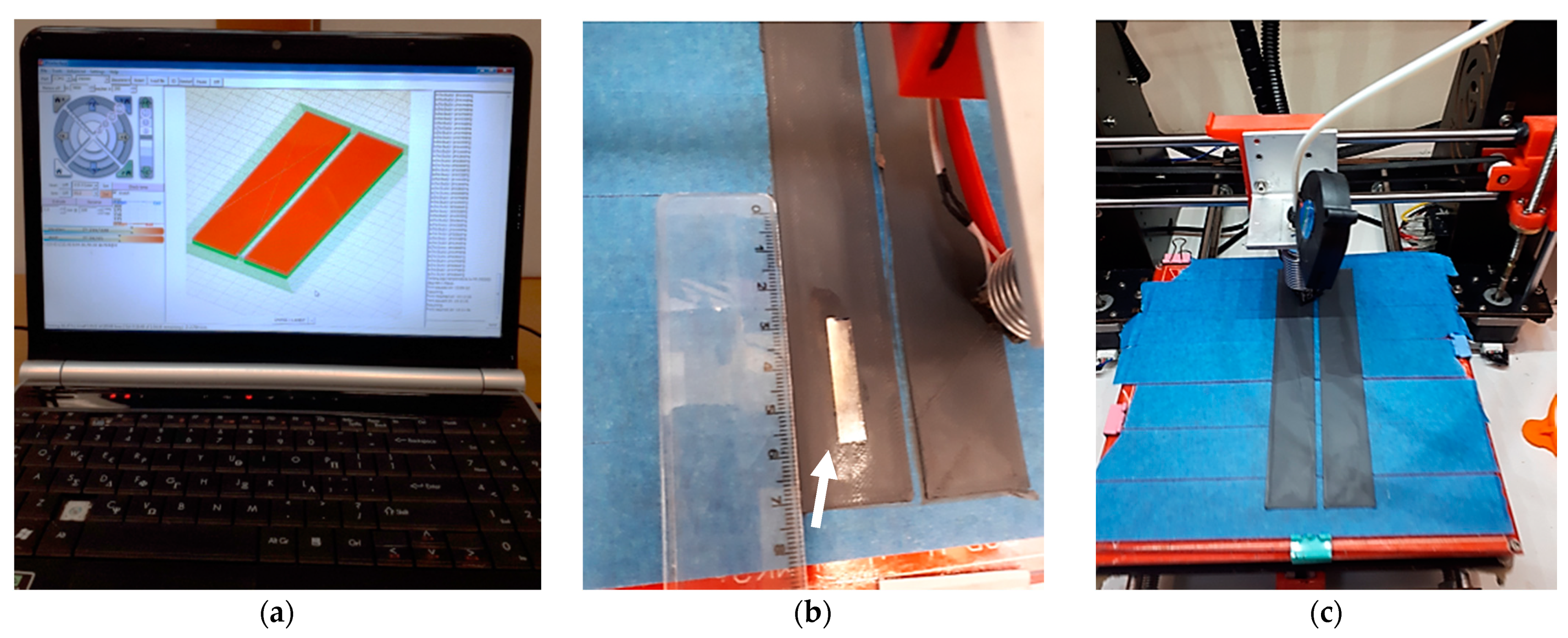
Rectangular slabs were prepared as in [19]. Briefly, the printer (CTC i3, Zhuhai Electronic Ltd., Zhuhai City, Guangdong, China) operated in fused deposition modeling (FDM) mode, had a single nozzle with a diameter of 0.4 mm, and used a polymer filament of 1.75 mm. The filament was a short carbon fiber reinforced PET-G polymer (CFRP) by 20 wt% (NEEMA3D™ Carbon: plus) of NEEMA3D™, Petroupolis, Greece. According to the manufacturer’s specifications, the filament’s Young’s modulus and Yield Strength were equal to E = 3800 MPa and 52.5 MPa, respectively. The printing temperature was set at 225 °C. Two slabs each measuring 170 × 25 × 3 mm³ were printed, one of which incorporated a 2826MB Metglas^® magnetoelastic (20 μm) strip of 25 × 5 mm², as sensing element. Another shorter slab (110 × 25 × 3 mm³) without sensing element was also printed. As described in [19], a sliced 3D design file was created for the considered slabs, and used in Pronterface^® software driving the 3D printer in Fused Deposition Mode (Figure 1a). The sensing element was easily incorporated during 3D-printing of slabs, by pausing the FDM printer once the desired layer height had been reached, so as to attach the strip with epoxy adhesive (Figure 1b). In the current case, 3D-printing of the slab in Figure 1b was temporarily halted when the slab’s thickness was equal to 1.75 mm. Then, the strip was attached and subsequently covered by successive material layers until obtaining the final slab thickness of 3 mm (Figure 1c).

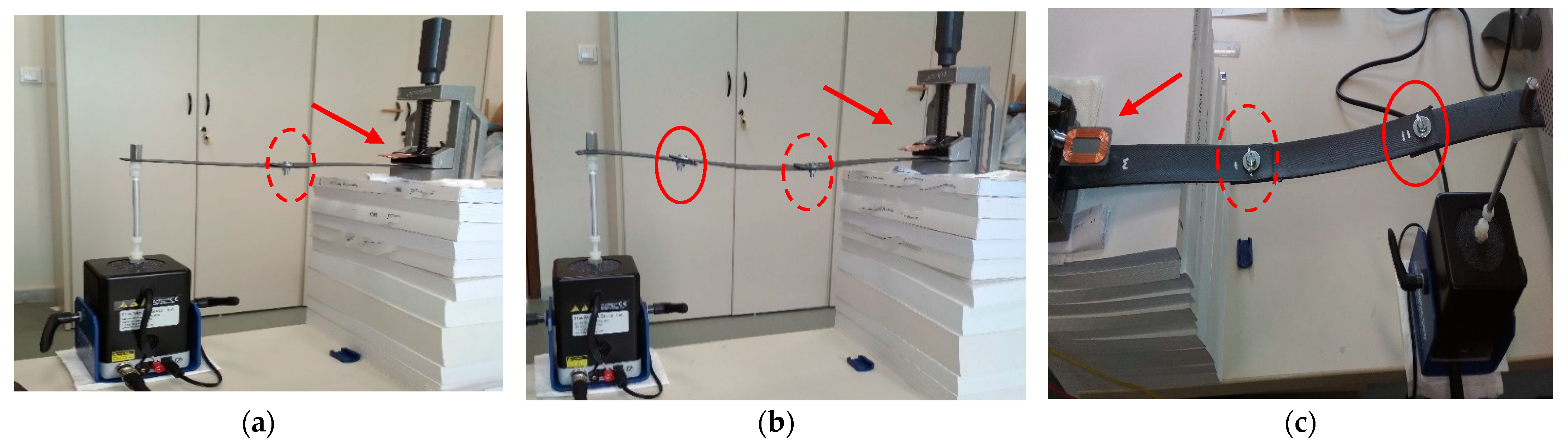
Two structures were formed by either two or three slabs connected in series with 5 mm bolts and washers, as shown in Figure 2. Since this study investigates the feasibility of modifying the framework in [19] for detecting and identifying failing joints, it seemed evident not to consider structures of complex geometry and numerous joints at this (initial) stage. Therefore, two basic structures were investigated: The first (most basic) one was used to verify that in case of issues with failing joints, the framework proposed in [19] in a suitably modified form, could detect the problem. The second structure should additionally allow for using the proposed framework to identify the joint that is failing. As seen in Figure 2, each joint between two slabs is formed with 5 mm bolts. This allowed for easily switching between a normal (tight) joint condition to a failing (loose) one after each test run. Hence, failing or normal conditions for a given joint were easily replicated, without having to dismantle the structure. Note that, the aim was to assess the operational condition of joints (fit for purpose, or not), rather than to pick up particular defects (i.e., breakage of adhesive film between surfaces, delamination problems) leading to compromised operation. This macroscopic approach, in turn, means that the proposed monitoring framework could be applicable to various kinds of joints (adhesive, bolted, etc.).

The structure with two slabs involves only one bolted joint and is referred to as structure-A (Figure 2a), whereas that with three slabs and, hence, two bolted joints is referred as structure-B (Figure 2b). Both structures are clamped as cantilevers at one end, whereas the free end is vibrated by means of a mini-exciter with integrated power amplifier (K2004E01, The Modal Shop, Cincinnati, USA). The latter is capable of producing various profiles of vibratory force/motion (triangular, sinusoidal, pulse-like, etc.) supplied by an external waveform generator (SDG 5122, SIGLENT). Structure-A measures 300 mm, and the bolted join (referred to as J1 and indicated by red dashed ellipsis in Figure 2a) is located 150 mm from the clamped end. Structure-B measures 400 mm and the two joints are located 150 mm (J1, indicated in Figure 2b by a red dashed ellipsis) and 300 mm (J2, indicated in Figure 2b by a red solid ellipsis) from the clamped end, respectively. In both structures, the slab involving the sensing element (MetGlas^® strip) is the one at the clamped end, as shown in Figure 2c.

As in [19], the response of the vibrating structure is translated into electrical signals created by induction to a low-cost reception coil (Vishay IWAS) placed at 20 mm above the slab incorporating the sensing element, as shown in Figure 2c. According to the principle explained in [19], the vibrational loading provokes changes in the magnetoelastic strip’s magnetization, which, in turn, causes induction of electrical signals in the reception coil circuits. Hence, this is a passive data transmission setup, in the sense that, unlike for instance [21,22], no excitation coil is used. All such signals were recorded by means of a conventional digital oscilloscope at 1 MHz. Note that the coil’s distance of 20 mm from the slab was defined by a trial-and-error process. In other words, the coil’s position comes from a trade-off obtained via an empirical process for recording signal output with principal frequency components of magnitude +20 to +30 dB over those of the noise layer.

2.2. Testing Procedure

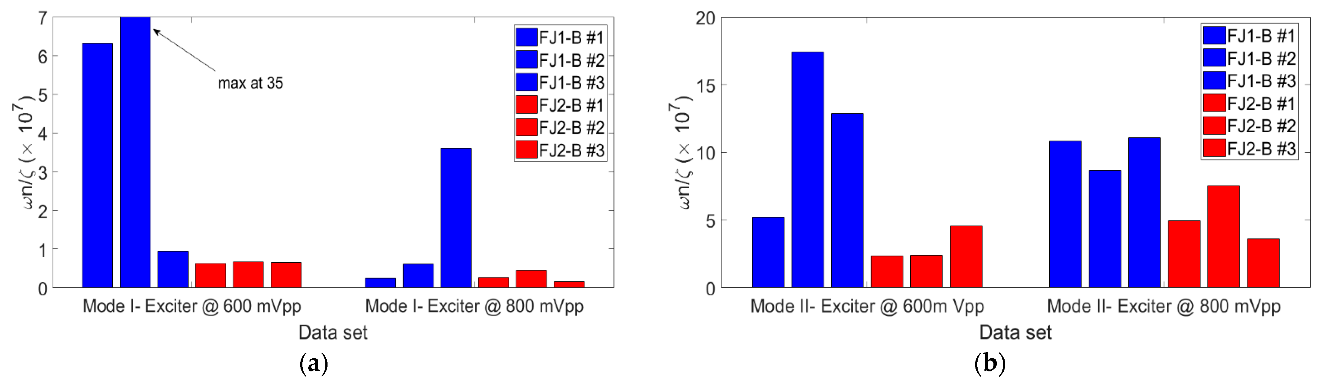
As explained in Section 2.1, the structure under test (structure-A or -B) is clamped at one end, whereas the other (free) end is attached to a stinger, i.e., a thin aluminum rod connected to the mini-exciter and shown on the left in Figure 2. Tests involve vibrating structure-A and -B at normal and at failing joint conditions. Normal joint conditions involve firmly fastened joints, obtained in the current case by applying a torque of up to 8 N/m. They are referred to as NJ-A for structure-A and NJ-B for structure-B. Failing joint conditions correspond to fastening the bolt using almost zero torque. Hence, even though the bolt bears contact with the washer, it is difficult to visually detect whether the joint is loose or not. For the same reason, the word “failing” is used (i.e., still operating in a substandard manner) and not “failed” (as for disrupted) joints. Failing J1 joint is referred to as FJ1-A or -B, for structure-A (Figure 2a) or structure-B (Figure 2b), respectively. On the other hand, only structure-B involves failing joints J2, which is a condition referred to as FJ2-B.

With respect to testing at failing joint conditions, structure-A may, obviously, be tested with only one failing joint (FJ1-A). Structure-B was tested with either J1 (FJ1-B) or J2 (FJ2-B) in failing condition. Test cases with two simultaneously failing joints (FJ1-B and FJ2-B) were not considered, since, in real life, identifying the first failing joint should call for applying remedial action to revert to a condition with tightly fastened joints. Note that, irrespectively of the location of the failing joint, excitation is always provided at the same point. This has not always been the case in structural vibration testing in the past. Since the excitation position does not have to be defined according to the location of the monitored joint, the current framework could be used with vibration data recorded from normal operation/loading of the structure.

As explained in Section 2.1, the starting point for producing a vibratory force from the mini-exciter is the definition of an initial suitable profile in the waveform generator. This is then used for driving the mini-exciter, which theoretically produces a force/motion profile matching the characteristics of the supplied waveform. In practice, this profile is somewhat different due to mechanical constraints (inertia of stinger and various internal parts, possibility of saturating actuators), bandwidth limitations of the exciter’s armature response, parasitic loading from the stinger’s off-centered motion during its operation etc. With respect to the profile of the initial waveform, a repetitive triangular form was preferred to pulses or perfect sinusoids. The reason is that loading profiles produced in several real-life cases rarely correspond to pulses or perfect sinusoids, with examples involving loading from people walking on the surface (not at a marching pace), or from operating machinery with rotating parts (internal combustion engines, for instance). On the other hand, with respect to selecting the waveform’s frequency, the aim was to produce mechanical force/motion of low amplitude and frequencies corresponding to those from operation of machinery with rotating parts. Initially, tests were intended to be performed at 20–40 Hz, which is roughly the case of an internal combustion engine rotating quite slowly at 1200–2400 rpm. Following tests with the waveform generator, it soon became clear that frequency components of 50 Hz of quite significant magnitude were always present, even for triangular waveforms of 20 Hz. This meant that testing at frequencies over 50 Hz was the only dependable scenario. In practice, selecting a frequency of 80 Hz for the triangular waveform means that the mini-exciter should be ultimately producing mechanical force at somewhat lower frequencies (due to reasons stated at the beginning of this paragraph), which would roughly correspond to an engine turning at mid-range (4000–4500 rpm).

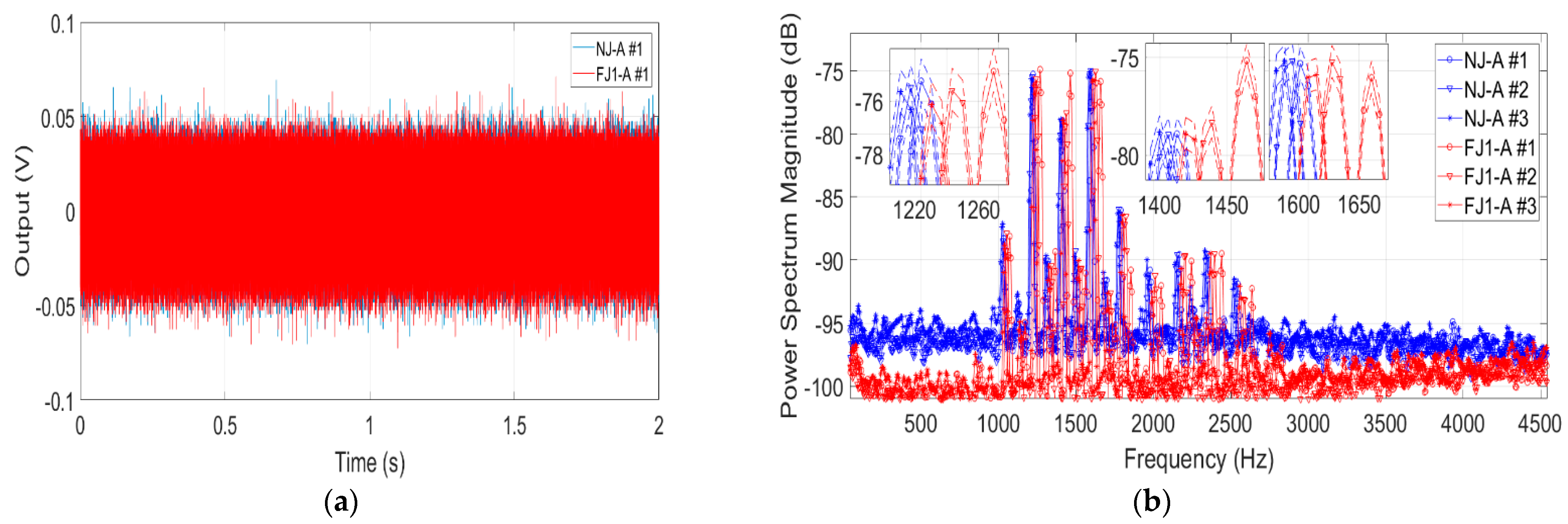
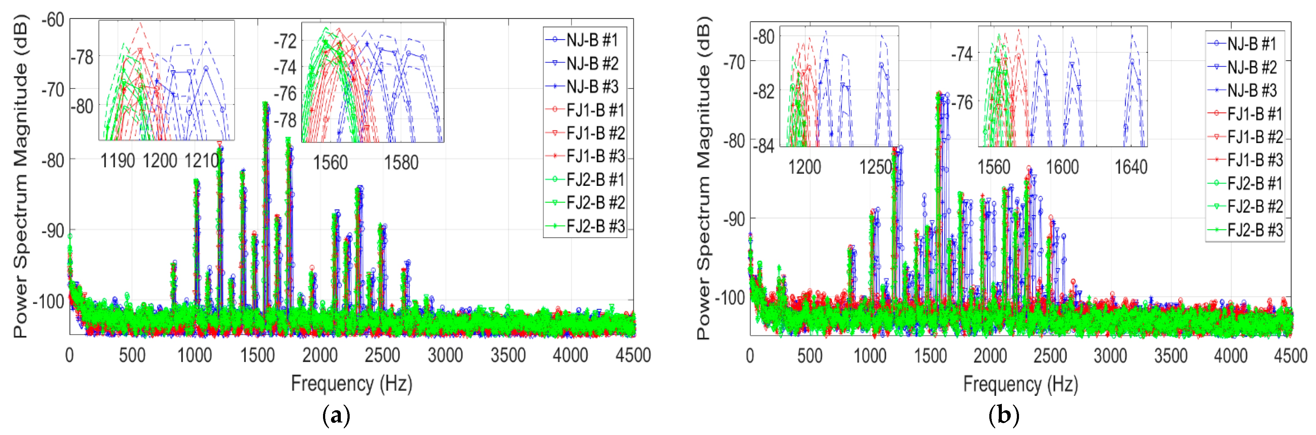
Hence, a triangular excitation profile at 80 Hz and 600 or 800 mVpp was selected in the waveform generator in order to drive the exciter. Note that, when a test was completed, the excitation input provided to the structure by the exciter was not recorded. Only output data recorded by the reception coil are used for detecting and identifying failing joints. This also means that, in principle, even test data from normal operation of the structure may be used for such monitoring purposes. All recorded signals underwent power spectrum analysis via the Welch method, with results presented in Section 3.

2.3. Second-Order Approximation Procedure for Damping Factor Estimation

There are two issues, which require further investigation before attempting to adapt the contactless diagnosis principle of [19] to the current application. First, the possibility of a failing joint quite far from the sensing element, which was not a problem in [19] since only one slab was involved; second, a significant variability in dynamics (following occurrence of a failing joint) of a structure formed from a group of slabs as opposed to dynamics of a single (continuous) slab. When system testing and recording of experimental data is completed, examination of the data frequency content usually leads to analyzing the most prominent modes, approximately corresponding to the most visible peaks in the plots (as already verified via finite element analysis in [19]). According to [20], chapter 10, such peaks in Frequency Response Function (FRF) plots may be attributed to complex pairs of system poles with very low values of damping factors. In essence, mapping peaks to pairs of lightly damped poles means that the response of the linear system is due to the superposition of responses of elementary under-damped second order systems. In other words, this principle is similar to partial fraction expansion (see [23], p. 61) usually performed in linear systems, with higher order systems decomposed to a series of first and second order systems for calculating the system response signal.

Thus, for such cases [20] proposes an empirical method to estimate the value of damping factor ζ for such pairs of lightly damped poles, based on the value ωn of the mode’s frequency, its peak magnitude in dB, and the half-power frequency values. These are two frequency values for which the mode’s magnitude reaches 70.7% of its peak, before (ωn_b) and after (ωn_a) frequency ωn. Using this set of points, the unknown damping factor value is computed as equal to 0.5 × (ωn_a − ωn_b)/ωn (see [20] for further details). This method is nicely suited to data characterized by low noise-to-signal ratio, but hardly suitable for many real-life noisy signals. In such cases, only peaks of modes of lightly damped pole pairs may be visible over the underlying noise in plots. Then, half-power frequencies ωn_b and ωn_a cannot be easily defined, since they are masked by the noise. Another issue is that very often the excitation input is not available. This is typically the case of recorded system responses not resulting from a dedicated experiment, but rather from system operation in typical real-life conditions. Then, for such output only systems, only power spectrum plots of the output signal may be available for estimation.

Therefore, a modification of this procedure is postulated in order to circumvent the noise masking effects. Each monitored peak of magnitude Mn and frequency ωn is still considered as resulting from a lightly damped complex pair of poles. Let the group of q spectrum points with frequencies be defined as [ω1, ω2, …, ωn, … ωq] and let [M1, M2, …, Mn, …, Mq] be the group of the associated magnitudes. Spectrum points ωi and Mi with i = 1…q and I ≠ n, are all points preceding and following the peak [ωn, Mn] of interest, that are still visible over the noise layer in spectrum plots. The effort, now, is to identify the second order system producing a peak that matches the monitored one at all points ωi and Mi with i = 1…q. This second-order approximation procedure is formulated as an iterative nonlinear optimization problem, as follows:

• Create the power spectrum plot of recorded data, define the value of resonant frequency ωn of the mode under examination, as well as the set of spectrum points [ω_i, M_i], i = 1…q on either side of ωn, which can be distinguished over the noise;
• Choose a set of parameters, namely the static gain A and damping factor ζ, for the trivial second order system with transfer function {A∙ωn²/(s² + 2∙ζ∙ωn∙s + ωn²)}, obtain its discrete time counterpart and estimate the power spectrum (using the same settings as in step 1) of the output to a given periodic input (preferably white noise);
• Focusing on frequencies ω_i, i = 1…q (see step 1), compute the quantity:

  $$r\left(k\right)={{\displaystyle \sum }}_{i=1}^q{\left[{\mathrm{M}}_i-M_i\right]}^2$$

  (1)

  at the k-th iteration, with M_i the magnitude of the power spectrum estimate of the second order system at ω_i;
• Go back to step 2, pick up a new set of A and ζ, and proceed to the next iteration by repeating steps 3 and 4, until a value of k for which r(k) becomes minimal is reached. Then, store the value for damping factor ζ, which corresponds to that of the considered (and monitored) mode.

This minimization procedure may be carried out by means of relevant nonlinear least squares routines, readily available in most software packages. For instance, in MATLAB^® one may use the command lsqnonlin.m for this purpose. During testing of the second-order approximation, simulations were carried out with higher order linear systems, which were driven with periodic input usually of triangular or sawtooth forms. Use of the second-order approximation procedure led to quite accurate results when dealing with modes with damping factor values lower than 10⁻³.

Finally, note that, as its name suggests, this procedure is intended as a means of approximating the true dynamics associated to a mode. In other words, it may not be used as a substitute for stochastic system identification procedures, which, as also demonstrated in [19], are extremely effective in capturing the global system dynamics. The only problem with system identification procedures is that identifying an effective and accurate system model requires significant user expertise and time for choosing the correct model structure. Hence, for a given set of signals, when rapid evaluation of a specific mode is necessary, then one may proceed with [20] or the currently presented second-order approximation procedure.

3. Experimental Results, Analysis and Discussion

The testing procedure described in Section 2.2 was applied to structure–A and –B for detecting failing joints and identifying those that are failing, where applicable. Three test runs for each configuration of structure-A (NJ-A, FJ1-A) and structure-B (NJ-B, FJ1-B, FJ2-B) were conducted, with the exciter driven by a triangular signal at 80 Hz and an amplitude of 600 mVpp (structure-A and –B) and 800 mVpp (structure-B). The case of detecting failing joints in a structure is treated in Section 3.1. It is shown that, in general, shifted frequency for specific modes observed in the power spectrum of structure response may be indicative of failing joints. The case of identifying the particular joint that is failing is treated in Section 3.2. It is shown that the task of failing joint identification is more complicated than the detection task of Section 3.1. For the identification task, both damping factor and shifted frequency characteristics should be simultaneously evaluated by using a specific feature defined in Section 3.2.

3.1. Detection of Failing Joint

As explained in Section 2.2, the testing protocol involved using the waveform generator to create a suitably selected signal (triangular with amplitude of 600 Vpp and frequency equal to 80 Hz) and driving the mini-exciter with it. Then, following vibration of structure-A or -B for the configurations described in Section 2.2, the output signal created in the reception coil circuit was recorded by means of an oscilloscope. Past experience with similar testing setups [19] suggested that there should be no visible differences between signal time histories from structures with normally fastened or failing joints. This proved again true and may be noted for structure-A in Figure 3a. The main reason for this characteristic is that, in such passive setups (i.e., without excitation of the reception coil) with signal transmission carried out in a contactless manner, the external mechanical loading cannot generate significant electrical power via the magnetoelastic phenomenon. Accordingly, it is difficult to produce response signals with variance visibly larger than that of the noise. Furthermore, due to the principle of contactless reception/recording of data, it is difficult to avoid noise in data, or issues such as significant total harmonic distortion (THD) values or spectrum intermodulation. This last issue can also be traced to specific magnetic properties (hysteresis loop) of materials such as MetGlas^® used in the current case for contactless transmission/reception purposes. Thus, one should be assessing specific qualitative rather than quantitative changes in the recorded signals. This means that only changes in their spectral characteristics could point to the original structure being affected by some kind of failure, which in the current case is a failing joint.

The case of test data from structure-A is presented in Figure 3b, with the inset showing the three largest peaks (modes). The previous comments on noise and significant total harmonic distortion values (estimated between 18.66% and 35.25% for 50 harmonics with data from all test cases in

Table 1. Testing scenarios (at 80 Hz–600 mVpp) for detecting failing joints in structure-A.

Test Case—Run #	Mode—I		Mode—II		Mode—III
	ζ	ωn (Hz)	ζ	ωn (Hz)	ζ	ωn (Hz)
NJ-A #1	6.28 × 10−4	1224	7.85 × 10−4	1412.5	2.37 × 10−4	1601.5
NJ-A #2	2.91 × 10−4	1217.5	4.62 × 10−4	1406.25	4.98 × 10−4	1595.1
NJ-A #3	7.35 × 10−4	1211	7.49 × 10−4	1399.7	5.92 × 10−4	1588.5
FJ1-A #1	2.49 × 10−4	1269.6	1.83 × 10−4	1464.5	2.98 × 10−4	1660
FJ1-A #2	3.18 × 10−4	1244	3.85 × 10−4	1438.8	9.94 × 10−5	1629.1
FJ1-A #3	1.63 × 10−4	1230.5	1.26 × 10−4	1419.3	2.38 × 10−5	1614.5

) seem valid. There is a clear shift in frequency values of modes around 1200, 1400 and 1600 Hz. The exact values of frequencies and the associated damping factors estimated by means of the second-order approximation (see Section 2.3) may be found in Table 1. Clearly, structure-A with normally fastened joints shows peaks at lower frequencies than those produced when joint J1 is failing. This behavior is probably due to the fact that failing joints cause low static friction between two contacting slab surfaces, thus allowing for relative displacement (rubbing) between them. Hence, the initial system with two firmly connected slabs becomes a group of two loosely connected slabs and this leads to frequency shifting phenomena at some frequencies. Another characteristic may be noted by examining the damping factor values in Table 1. Damping values resulting from structure-A with failing joints are generally lower than those from structures with normally secured joints, and this is particularly true for Modes II and III. Note that the second-order approximation procedure yields results in about 6 min for each considered mode. This time interval is significantly shorter than that required for identifying a system model equivalent, for instance, to that in [19]. An indication of the second order approximation’s accuracy is provided by the quantity √r(k)/q (see Section 2.3—step 3), which essentially shows the mean distance between the spectrum of the second order system and that from test data for the monitored mode. Values for this quantity are quite low (ranging from 0.17 to 0.43 dB per parameter) and indicate successful approximation. Furthermore, an additional remark on the standard deviation of the spectra presented in Figure 3b may be formulated. In fact, the upper and lower limits of the curves presented in Figure 3b (corresponding to the confidence intervals for those curves at 95% level) indicate that there are quite small differences of up to ±1.3 dB, for peak magnitudes generally ranging between −75 and −80 dB. These narrow intervals suggest that it is reasonable to estimate damping factor values by applying the second order approximation to power spectrum curves such as those in Figure 3b.

The same remarks are valid for tests with structure-B, again with data exhibiting significant noise and total harmonic distortion characteristics (with relevant values between 13.75% and 27.74% for 50 harmonics estimated with test data from cases in

Table 2. Testing scenarios (at 80 Hz–600 mVpp) for detecting and identifying failing joints in structure-B.

Test Case—Run #	Mode—I			Mode—II
	ζ	ωn (Hz)	ωn/ζ	ζ	ωn (Hz)	ωn/ζ
NJ-B #1	6.754 × 10−5	1211	n/a	2.936 × 10−6	1584	n/a
NJ-B #2	1.443 × 10−4	1205	n/a	2.741 × 10−5	1577	n/a
NJ-B #3	2.249 × 10−4	1201	n/a	1.764 × 10−5	1569	n/a
FJ1-B #1	1.898 × 10−5	1197.5	63,092,729.18	3.017 × 10−5	1566.5	51,922,439.51
FJ1-B #2	3.510 × 10−6	1195.1	340,484,330.48	9 × 10−6	1563	173,666,666.67
FJ1-B #3	1.263 × 10−4	1195	9,461,599.37	1.217 × 10−5	1561.5	128,307,313.06
FJ2-B #1	1.920 × 10−4	1193	6,213,541.67	6.636 × 10−5	1558	23,477,998.79
FJ2-B #2	1.782 × 10−4	1191	6,683,501.68	6.54 × 10−5	1558	23,822,629.97
FJ3-B #3	1.822 × 10−4	1191	6,536,772.78	3.418 × 10−5	1558	45,582,211.82

). Figure 4a presents the frequency characteristics of structure-B for the configurations described in Table 1, with the exciter driven by a triangular signal with amplitude of 600 mVpp and frequency of 80 Hz. Again, structure-B with normally secured joints produces data with peaks at higher frequencies than those from slabs with failing joints. The exact values of frequencies and the associated damping values estimated by means of the second-order approximation may be found in Table 2. Focus is now given on the two largest peaks of the spectrum plot, since the third and fourth peaks are roughly of equivalent magnitude. This property of shifted frequencies is consistent for the two largest peaks (modes) in the power spectrum plot, but a trend opposite to that shown in Figure 3b is noted. Data from structures with failing joints have modes at lower frequencies than data from structures with normally fixed joints, unlike what is observed in Figure 3b. Since this could create doubts about a poorly executed set of test runs and/or some inappropriate setting, another set of test runs now with the exciter driven by a triangular signal at 80 Hz but with an amplitude of 800 mVpp was conducted. Again, data exhibited significant noise and total harmonic distortion characteristics (with relevant values between 20.97% and 26.87% for 50 harmonics estimated with test data from cases in

Table 3. Testing scenarios (at 80 Hz–800 mVpp) for detecting and identifying failing joints in structure-B.

Test Case—Run #	Mode—I			Mode—II
	ζ	ωn (Hz)	ωn/ζ	ζ	ωn (Hz)	ωn/ζ
NJ-B #1	5.783 × 10−5	1255.5	n/a	1.934 × 10−5	1641.7	n/a
NJ-B #2	3.091 × 10−4	1228.6	n/a	7.567 × 10−6	1606.3	n/a
NJ-B #3	2.530 × 10−4	1213.3	n/a	8.866 × 10−5	1587.3	n/a
FJ1-B #1	4.735 × 10−4	1204.1	2,542,977.82	1.114 × 10−5	1576	108,087,971.3
FJ1-B #2	1.937 × 10−4	1197.9	6,184,305.62	1.384 × 10−5	1566.7	86,553,468.21
FJ1-B #3	3.316 × 10−5	1194.7	36,028,347.41	1.080 × 10−5	1563	110,620,370.4
FJ2-B #1	4.512 × 10−4	1192.4	2,642,730.49	2.405 × 10−5	1558.6	49,580,041.58
FJ2-B #2	2.692 × 10−4	1196.2	4,443,536.40	1.589 × 10−5	1564.4	75,280,050.35
FJ3-B #3	7.293 × 10−4	1195.6	1,639,380.22	3.313 × 10−5	1564.6	36,088,137.64

). Results proved very similar to those already available (obtained with the exciter driven at 600 mVpp) and may be seen in Figure 4b. The exact values of frequencies and the associated damping values estimated by means of the second-order approximation may be found in Table 3. In all runs, values for √r(k)/q (see Section 2.3—step 3) range between 0.19 and 0.46, thus indicating successful approximation of the considered spectra. When joints are failing in structure-B, spectrum modes are shifted to lower frequencies than those corresponding to structure-B with normally fastened joints. This observation illustrates the variable behavior in dynamics of structures with respect to those of single continuous bodies, and the relevant comment at the beginning of Section 2.3.

Note that the same remark on the confidence intervals (at 95% confidence level) of the spectra presented in Figure 4 may be formulated for tests carried out with structure-B. There are quite small differences of up to ±1.3 dB for magnitudes generally peaking between −75 and −85 dB. Thus, one may reasonably use the power spectrum curves presented in Figure 4 for estimating damping factor values by means of the second order approximation. Hence, detecting a structure with failing joints is a task which is possible to perform by carrying out several tests at NJ-A or NJ-B configurations for delimiting frequency ranges of specific main modes, and looking for shifted mode frequencies during the structure’s inspection.

3.2. Identification of the Failing Joint

Obviously for a structure involving more than one joint, the main goal is to identify the one that is failing. For this purpose, data from tests with structure-B and specifically, damping factors and frequencies of the (two) modes shown in Table 2 and Table 3 may be used as follows. From Figure 4 it is obvious that data resulting from FJ1-B tests feature broadly similar frequencies to those resulting from FJ2-B tests for the modes considered. But damping factors for these two modes are consistently higher for data resulting from FJ2-B tests than those from FJ1-B tests. This observation is significant but of rather limited practical interest. In fact, a conclusion on whether J1 or J2 is failing should be drawn based on setting thresholds for a single quantity, as opposed to using some combinatory reasoning. Ideally, one should include values of frequencies and damping factors into one feature, which should offer a clear indication as to which joint is failing.

To introduce such a feature, one may attempt the following reasoning. The mode considered is thought of as corresponding to a trivial second order system like the simple harmonic oscillator in Figure 5. This is essentially a mass m moving due to the application of an external force f(t) while restricted by a spring of constant K and a damping element of constant C (also known as mass-spring-damper system, see Chapter 2 in [23]). Its resonant ωn and damping factor ζ may be easily computed (see Chapter 2, ref. [23]) as:

$$\omega n=\sqrt{\frac{K}{m},}\zeta =\frac{C}{2·\sqrt{K·m}}$$

(2)

The feature ωn/ζ depends only on the ratio between K and C. In other words, the ratio ωn/ζ associates both damping and stiffness characteristics into a single quantity, which responds to variations in either K or C. Specifically, if the resonant frequency of the considered mode varies little between data sets, the feature ωn/ζ is highly sensitive to damping variations.

Computing this feature for data in Table 2 and Table 3 reveals that data from FJ2-B tests show lower values than those obtained from FJ1-B tests, as exhibited in bar plots of Figure 6. For data sets produced with the exciter driven at 80 Hz and 600 mVpp, all values for ωn/ζ are clearly (and consistently) lower for FJ2-B tests in mode I (Figure 6a) than those obtained for FJ1-B tests. This trend remains, albeit not with the same consistency, for values of ωn/ζ in mode II (Figure 6b). The case of data sets produced with the exciter driven at 80 Hz and 800 mVpp is a bit different due to the value of ωn/ζ for test FJ1-B #1 being abnormally low and comparable to values obtained for FJ2-B test data in mode I (Figure 6a). But, even then all values of ωn/ζ for FJ2-B test data are consistently low. In mode II, values for ωn/ζ are lower for FJ2-B tests, as for the case of the exciter being driven at 600 mVpp (Figure 6b). Hence, identifying the joint that is failing is a task which is possible to be based on: (i) performing tests during the structure’s inspection phase; (ii) approximating damping factors of specific modes by means of the second-order approximation (in Section 2.3); (iii) computing values of feature ωn/ζ, and comparing with past results.

Note that results are obtained without dismantling the tested structures and/or separately examining each joint by means of dedicated equipment [10,11,12,13]. Consequently, the currently obtained results describe whether a joint is fit for purpose or not, and do not provide explanation on the origins of failure (as is the case for [10,11,12,13]). The current framework operates by estimating spectral characteristics of the structure’s response to testing via simple algorithmic procedures (i.e., the second order approximation) and specific features (ωn/ζ). In that sense, the proposed framework operates in a similar manner to vibration-testing based techniques [18,19] and achieves similar results but without the associated cost in terms of equipment (accelerometers, amplifiers [18]) or modelling expertise required for the user [19].

4. Conclusions

This study proposes a comprehensive framework for monitoring the condition of joints in structures with composite members/components, by extending the methodology proposed for single (continuous) slabs in [19]. Testing was based on low-frequency vibration loading used for inspecting metal structures [18], but also for monitoring adhesively bonded sandwich joints [12]. With respect to previous relevant approaches, the key element of the current framework is that the structure is excited at a standard location irrespectively of the monitored joint. Then, even data from normal structure operation may be utilized for monitoring purposes, thus avoiding “off duty” periods for carrying out testing. Care has been taken to use conventional equipment as far as possible both for data recording and for analysis purposes. Therefore, 3D-printing processes were used for incorporating magnetoelastic sensing elements in one of the composite members/components of the structure. Then, a reception coil suspended above that member/component was used for recording the response of the structure under vibration in a contactless manner. This allows for recording data without using amplifiers or accelerometers. The data analysis part has also been modified with respect to previous studies [19], aiming at delivering results without requiring significant expertise from the user. For this purpose, a method for assessing the frequency characteristics of the response signal was presented. Its main novelties include a quick iterative approach for estimating damping factors of selected modes and a methodology for performing detection of possibly failing joints and identification of the joint that is failing. For the latter, a feature sensitive to frequency and damping variations from failing joints was defined and used for distinguishing between all joints that were candidates for failing. The framework has been tested with two structures and has been found to perform in a promising manner. Further development of the proposed framework involves its tuning for application to structures with multiple joints and complex geometry, as well as the introduction of additional features for identifying the joint that is failing among a given number of candidates.

References

1. Mouzakis, D.E. Advanced technologies in manufacturing 3D-layered structures for defense and aerospace. In Lamination—Theory and Application; Osheku, C.A., Ed.; IntechOpen Press: London, UK, 2018; pp. 89–113. Available online: https://www.intechopen.com/books/lamination-theory-and-application/advanced-technologies-in-manufacturing-3d-layered-structures-for-defense-and-aerospace (accessed on 30 March 2021). [CrossRef] [Green Version]
2. Dimogianopoulos, D.G.; Mouzakis, D.E. A Versatile Interrogation-Free Magnetoelastic Resonator Design for Detecting Deterioration-Inducing Agents. In Lecture Notes in Civil Engineering 110, Proceedings of 1st International Conference on Structural Damage Modelling and Assessment SDMA 2020, Ghent University, Belgium, 4–5 August 2020; Abdel Wahab, M., Ed.; Springer: Singapore, 2021; pp. 113–119. [Google Scholar] [CrossRef]
3. Kocherla, A.; Duddi, M.; Subramaniam, K.V.L. Smart Embedded PZT Sensor for In-Situ Elastic Property and Vibration Measurements in Concrete. Measurement 2021, 173, 108629. [Google Scholar] [CrossRef]
4. Quattrocchi, A.; Freni, F.; Montanini, R. Self-Heat Generation of Embedded Piezoceramic Patches Used for Fabrication of Smart Materials. Sens. Actuator A Phys. 2018, 280, 513–520. [Google Scholar] [CrossRef]
5. Sousa, J.; Marques, J.; Garcia, M.; Infante, V.; Amaral, P. Mechanical Characterization of Sandwich Composites with Embedded Sensors. Eng. Fail. Anal. 2020, 117, 104765. [Google Scholar] [CrossRef]
6. Rupp, H.; Binder, W.H. Multicomponent Stress-Sensing Composites Fabricated by 3D-Printing Methodologies. Macromol. Rapid Commun. 2021, 42, 2000450. [Google Scholar] [CrossRef] [PubMed]
7. Moheimani, R.; Agarwal, M.; Dalir, H. 3D-Printed Flexible Structures with Embedded Deformation/Displacement Sensing for the Creative Industries. In Proceedings of the AIAA Scitech 2021 Forum, Virtual Event. 11–15 & 19–21 January 2021; p. 0534. [Google Scholar] [CrossRef]
8. Yun, S.M.; Kim, M.; Kwon, Y.W.; Kim, H.; Kim, M.J.; Park, Y.G.; Park, J.U. Recent Advances in Wearable Devices for Non-Invasive Sensing. Appl. Sci. 2021, 11, 1235. [Google Scholar] [CrossRef]
9. Ryan, K.R.; Down, M.P.; Banks, C.E. Future of Additive Manufacturing: Overview of 4D and 3D Printed Smart and Advanced Materials and Their Applications. Chem. Eng. J. 2021, 403, 126162. [Google Scholar] [CrossRef]
10. Qi, X.F.; Yang, Y.; Kang, W.P.; Wang, Q.; Zhao, G. On-line Monitoring by Acoustic Emission of Butt Joint Structure on the Composite Fuselage Frame. In IOP Conf. Series: Materials Science and Engineering 739, Proceedings of the 2019 6th International Conference on Advanced Materials, Mechanics and Structural Engineering, Seoul, Korea, 18–20 October 2019; Springer: Seoul, Korea, 2020; p. 012043. [Google Scholar]
11. Barile, C.; Casavola, C.; Pappalettera, G.; Vimalathithan, P.K. Multiparameter Approach for Damage Propagation Analysis in Fiber-Reinforced Polymer Composites. Appl. Sci. 2021, 11, 393. [Google Scholar] [CrossRef]
12. Khosravani, M.R. Influences of Defects on the Performance of Adhesively Bonded Sandwich Joints. Key Eng. Mater. 2018, 789, 45–50. [Google Scholar] [CrossRef]
13. Santos, M.A.S.; Campilho, R.D.S.G. Experimental and Numerical Analysis of the Fracture Envelope of Composite Adhesive Joints. Sci. Techn. Mater. 2018, 30, 131–137. [Google Scholar] [CrossRef]
14. Rucka, M.; Wojtczak, E.; Lachowicz, J. Damage Imaging in Lamb Wave-Based Inspection of Adhesive Joints. Appl. Sci. 2018, 8, 522. [Google Scholar] [CrossRef] [Green Version]
15. Schroeder, J.A.; Ahmed, T.; Chaudhry, B.; Shepard, S. Non-Destructive Testing of Structural Composites and Adhesively Bonded Composite Joints: Pulsed Thermography. Compos. Part A Appl. Sci. Manuf. 2002, 33, 1511–1517. [Google Scholar] [CrossRef]
16. Yi, Q.; Tian, G.Y.; Yilmaz, B.; Malekmoha Mmadi, H.; Laureti, S.; Ricci, M.; Jasiuniene, S. Evaluation of Debonding in CFRP-Epoxy Adhesive Single-Lap Joints Using Eddy Current Pulse-Compression Thermography. Compos. B Eng. 2019, 178, 107461. [Google Scholar] [CrossRef]
17. Wang, B.; Zhong, S.; Lee, T.L.; Fancey, K.S.; Mi, J. Non-Destructive Testing and Evaluation of Composite Materials/Structures: A State-Of-The-Art Review. Adv. Mech. Eng. 2020, 12, 1–28. [Google Scholar] [CrossRef] [Green Version]
18. Salgado Sánchez, P.; López Negro, P.; García-Fogeda, P. Vibration-Based Method for Damage Detection at Welded Beams and Rods. Lat. Am. J. Solids Struct. 2016, 13, 2336–2355. [Google Scholar] [CrossRef] [Green Version]
19. Dimogianopoulos, D.G.; Charitidis, P.J.; Mouzakis, D.E. Inducing Damage Diagnosis Capabilities in Carbon Fiber Reinforced Polymer Composites by Magnetoelastic Sensor Integration via 3D Printing. Appl. Sci. 2020, 10, 1029. [Google Scholar] [CrossRef] [Green Version]
20. Rao, S.S. Mechanical Vibrations, 5th ed.; Prentice Hall: Hoboken, NJ, USA, 2011; pp. 908–915. [Google Scholar]
21. Ren, L.; Yu, K.; Tan, Y. Applications and Advances of Magnetoelastic Sensors in Biomedical Engineering: A Review. Materials 2019, 12, 1135. [Google Scholar] [CrossRef] [PubMed] [Green Version]
22. Grimes, C.A.; Jain, M.K.; Singh, R.S.; Cai, Q.; Maso, A.; Takahata, K.; Gianchandani, Y. Magnetoelastic microsensors for envinronmental monitoring. In Proceedings of the IEEE International Conference on Micro Electro Mechanical Systems (MEMS), Interlaken, Switzerland, 21–25 January 2001. [Google Scholar] [CrossRef]
23. Dorf, R.C.; Bishop, R.H. Modern Control Systems, 12th ed.; Prentice Hall: Upper Saddle River, NJ, USA, 2010. [Google Scholar]
Figure 1. (a) Detail of the 3D design file used with Pronterface® software, which drives the 3D printing process in fused deposition modelling mode; (b) Fixing of the Metglas® strip (indicated by white arrow) via epoxy adhesive whilst 3D printing is temporarily halted (slab is 1.75 mm thick at that point); (c) continuation of material layering until a slab thickness of 3 mm is reached.
Applsci 11 03230 g001
Figure 2. (a) Structure-A formed by two slabs connected in-series and clamped at one end; (b) Structure-B formed by three slabs connected in-series and clamped at one end; (c) top view of structure-B showing locations of MetGlas® strip (marked with Σ) and the bolts (marked with I and II, respectively) of joints J1 and J2. The reception coil (indicated by red arrows) is suspended above the strip position, J1 and J2 are indicated by red ellipses (dashed-solid, respectively) and the free end is supported/vibrated via the mini-exciter.
Applsci 11 03230 g002
Figure 3. Output signals from test runs with structure-A for the configurations in Section 2.2: (a) Typical time histories of NJ-A versus FJ1-A showing no visible differences; (b) Spectra of NJ-A versus FJ1-A showing clear frequency shifts for the three largest modes due to failing joint. Dashed lines indicate confidence intervals at 95% level.
Applsci 11 03230 g003
Figure 4. Spectra of output signals from test runs with structure-B (see Section 2.2) with the exciter driven: (a) By triangular waveform at 80 Hz-600 mVpp and (b) By triangular waveform at 80 Hz-800 mVpp. Insets present spectra of NJ-B (in blue) versus FJ1-B (in red) or FJ2-B (in green) showing clear frequency shifts for the two largest modes due to failing joints. Dashed lines indicate confidence intervals at 95% level.
Applsci 11 03230 g004
Figure 5. The simple harmonic oscillator featuring a mass m, moving due to the external force f, while constrained by the damping element with constant C and the spring element with constant K. The oscillator’s natural frequency ωn and damping factor ζ are in Formula (2).
Applsci 11 03230 g005
Figure 6. Bar plots indicating the values of ωn/ζ for tests conducted with the exciter driven at 80 Hz with amplitude of 600 and 800 mVpp: (a) Mode I; (b) Mode II (see Table 2 and Table 3 for more information on modes).
Applsci 11 03230 g006